Partial Reset in Pulse-Coupled Oscillators

Abstract.

Pulse-coupled threshold units serve as paradigmatic models for a wide range of complex systems. When the state variable of a unit crosses a threshold, the unit sends a pulse that is received by other units, thereby mediating the interactions. At the same time, the state variable of the sending unit is reset. Here we present and analyze a class of pulse-coupled oscillators where the reset may be partial only and is mediated by a partial reset function. Such a partial reset characterizes intrinsic physical or biophysical features of a unit, e.g., resistive coupling between dendrite and soma of compartmental neurons; at the same time the description in terms of a partial reset makes possible a rigorous mathematical investigation of the collective network dynamics.

The partial reset acts as a desynchronization mechanism. For $N$ all-to-all pulse-coupled oscillators an increase in the strength of the partial reset causes a sequence of desynchronizing bifurcations from the fully synchronous state via states with large clusters of synchronized units through states with smaller clusters to complete asynchrony. By considering inter- and intra-cluster stability we derive sufficient and necessary conditions for the existence and stability of cluster states on the partial reset function and on the local dynamics of the oscillators, as specified by their rise function. This analysis of invariance and stability goes beyond monotonicity and curvature of the rise function and classifies the local dynamics according to certain expansion and contraction properties that depend also on the third derivative of the rise function. We obtain analytical bounds for the stability of cluster states and for a specific class of oscillators a rigorous derivation of all $N-1$ bifurcation points. Thus the sequence of bifurcation points is extensive (of the order of the system size $N$) with the actual number of bifurcating states growing combinatorially in $N$. We demonstrate that the entire sequence of bifurcations may occur due to arbitrarily small changes of the reset function. We illustrate that the transition is robust against structural perturbations and prevails in presence of heterogeneous network connectivity and rise functions with mixed curvature.

1. Introduction

Networks of pulse-coupled units serve as paradigmatic models for a wide range of physical and biological systems as different as cardiac pacemaker tissue, plate tectonics in earthquakes, chirping crickets, flashing fireflies and neurons in the brain [12, 11, 46, 7]. In such systems, units interact by sending and receiving pulses at discrete times that interrupt the otherwise smooth time evolution. These pulses may be sound signals, electric and electromagnetic activations as well as packets of mechanically released stress. Pulses are generated once the state of a unit crosses a certain threshold value (e.g. the mechanical stress of a tectonic plate becomes sufficiently large or the voltage across a nerve cell membrane becomes sufficiently high); thereafter the state of the sending unit is reset.

Synchronization of oscillators is one of the most prevalent collective dynamics in pulse-coupled systems [45, 21, 22, 8, 10, 30, 26, 27, 60]. Often not all units are synchronized but form clusters consisting of synchronized sub-groups of units which in turn are phase-locked to other clusters [21, 62, 44, 5, 30, 29, 40, 50, 51].

In neuronal networks synchronization and clustering of pulses constitute potential mechanisms for effective feature binding. In this paradigm, different information aspects of the same object represented by activity of different nerve cells are pooled together by temporal correlations and in particular due to synchronous firing [56, 57]. However, strong synchronized firing of nerve cells can also be detrimental: synchrony is prominent during epileptic seizures [18, 42] and observed in the basal ganglia during Parkinson tremor [17]. Here mechanisms for desynchronizing neural activity are desirable [59, 41].

To study key mechanisms that may underly synchronization, e.g. in biological neural networks, analytical tractable models of pulse-coupled oscillator are helpful tools [49, 45, 38, 1, 21, 8, 63, 15]. Here the rise of the state variable of a free oscillatory unit towards the threshold, the unit’s rise function characterizes the sub-threshold dynamics. If after reception of a pulse the state variable of the unit stays below threshold it is said to receive sub-threshold input, whereas excitation above the threshold is supra-threshold. Mirollo and Strogatz [45] showed that biological oscillators always synchronize their firing in homogeneous networks with excitatory all-to-all coupling if the rise function has a concave shape. The synchronization mechanism they find has two parts: (i) effective decrease of phase differences of units due to sub-threshold inputs and (ii) instant synchronization due to supra-threshold inputs and subsequent reset to a fixed value.

In general, supra-threshold excitation and a subsequent reset is a dominant mechanism for synchronization of pulse-coupled oscillators because input pulses that force non-synchronized units to cross threshold at nearby times are reset to the same value leaving the units in the same state or in very similar states afterwards. Although this reset mechanism plays a crucial role in the synchronization process and the coordination of pulse generation times, its implications for the collective network dynamics has - to our knowledge - not been investigated systematically so far: most existing model studies reset the units with supra-threshold inputs to a fixed value independent of the strength of supra-threshold excitation [6, 21, 38, 55, 62, 13, 15, 31]. This results in a complete loss of information about the prior state of the units and makes the dynamics non-invertible. Some other studies consider the opposite extreme: a complete conservation of supra-threshold inputs during pulse sending and reset [31, 8]. Here we aim at closing this gap by presenting and analyzing a model where the reset (and thus the loss of information about the prior state and the strength of supra-threshold excitation) can be varied systematically.

This article is organized as follows: In section 2 we propose a simple model of pulse-coupled oscillators with partial reset, where the response to supra-threshold inputs can be continuously tuned and is not an all-or-none effect. To isolate the consequences of partial reset, we focus on homogeneous systems of all-to-all pulse-coupled oscillators with convex rise function. In section 3 we briefly present the results of numerical simulations and find that the partial reset has a strong influence on the collective network dynamics: Increasing the strength of the partial reset induces bifurcations from the fully synchronous state via states with large clusters of synchronized units through states with smaller clusters to complete asynchrony. We study this transition rigorously by considering existence and stability periodic cluster states with respect to inter-cluster properties in section 3.4 and to intra-cluster properties in 3.5. We derive conditions on the partial reset function and the rise function to bound regions of existence and stability of cluster states. In 3.6 we present a rigorous derivation of $N-1$ bifurcation points for a specific class of oscillators. We demonstrate that the entire sequence of bifurcations may occur for arbitrarily small changes of the reset function, thus underlining the strong impact of partial reset on collective network dynamics. In section 4 we numerically illustrate that the transition is robust against structural perturbations and prevails in presence of heterogeneous network connectivity and rise functions with mixed curvature. In section 5 we discuss our results and relate the simple partial reset model to biophysically more realistic neuron models .

Specific aspects of the implications of linear partial reset on synchronization properties for oscillators have been briefly reported before [35].

2. Networks of Pulse-Coupled Units with Partial Reset

We first propose a class of pulse coupled threshold elements with partial reset and thereafter focus on units that oscillate intrinsically.

2.1. Absorption Rule and Instant Synchronization

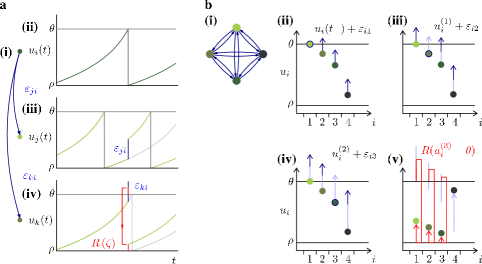
Figure 2.1. Model dynamics. (a) Sample traces of three units with (i) network connectivity $\varepsilon_{ji}=\varepsilon_{ki}>0$. (ii) At time $t=t_{1}$ unit $i$ reaches the threshold $\theta$ and its membrane potential is reset to $\rho$. It generates a pulse which is send to the units $j$ and $k$. (iii) unit $j$ receives the pulse and its membrane potential is increased to $u_{j}(t_{1}^{-})+\varepsilon_{ji}$, the pulse is sub-threshold. (iv) unit $k$ receives a supra-threshold pulse, $u_{k}(t_{1}^{-})+\varepsilon_{kj}\geq\theta$, its membrane potential is set to $R(\zeta)=R\left(u_{j}(t_{1}^{-})+\varepsilon_{kj}-\theta\right)$ using the partial reset function $R$. (b) Sample avalanche process with $\Theta=\left\{1,2,3\right\}$ and $n=3$ in (i) a $N=4$ all-to-all network $\varepsilon_{ij}=(1-\delta_{ij})\varepsilon$. (ii) unit $i=1$ reaches the threshold $\Theta^{(0)}=\left\{1\right\}$ and sends a pulse to the other units (arrows). Their potentials are updated to $u_{i}^{(1)}=u_{i}(t^{-})+\varepsilon_{i1}$, causing unit $i=2$ to generate a pulse, $\Theta^{(1)}=\left\{2\right\}$. (iii) The pulse is received by the other units yielding a potential $u_{i}^{(2)}=u_{i}^{(1)}+\varepsilon_{i2}$ which brings unit $i=3$ above threshold $\Theta^{(2)}=\left\{3\right\}$. (iv) The potentials become $u_{i}^{(3)}=u_{i}^{(2)}+\varepsilon_{i3}$ and no further unit crosses the threshold, $\Theta^{(3)}=\emptyset$. (v) The avalanche stops and units that received supra-threshold input are reset to $u_{i}(t)=\rho+R\left(u_{i}^{(3)}-\theta\right)$.

We consider $N$ threshold elements, which at time $t$ are characterized by a single real state variable $u_{i}(t)$ with $i\in\{1,2,\dots,N\}$. In the absence of interactions the state variables evolve freely according to the differential equation

(2.1) $$\frac{d}{dt}u_{i}=F\left(u_{i}\right)$$

with a smooth function $F:\mathbb{R}\rightarrow\mathbb{R}$ specifying the intrinsic dynamics of the units. The free dynamics are endowed with an additional nonlinear reset upon reaching a fixed threshold $\theta$ from below

(2.2) $$u_{i}\left(t^{-}\right)=\theta\quad\Rightarrow\quad u_{i}\left(t\right)=\rho$$

where $\rho<\theta$ is the reset value and we used the notation $u_{i}\left(t^{\pm}\right)=\lim_{s\searrow 0}u_{i}\left(t\pm s\right)$. By an appropriate shift and rescaling of the state variable and its dynamics we set $\rho=0$ and $\theta=1$ without loss of generality.

The units are $\delta$-pulse coupled. If unit $j$ reaches the threshold a pulse of strength $\varepsilon_{ij}\geq 0$ is send instantaneously to units $i$ and their membrane potential is increased by an amount $\varepsilon_{ij}$

(2.3) $$u_{j}\left(t^{-}\right)=\theta\quad\Rightarrow\quad u_{i}^{(1)}=u_{i}\left(t^{-}\right)+\varepsilon_{ij}$$

If there is no connection from unit $j\rightarrow i$ we set $\varepsilon_{ij}=0$.

If a unit $i$ crosses the threshold due to a pulse from unit $j$

(2.4) $$u_{i}\left(t^{-}\right)+\varepsilon_{ij}\geq\theta$$

it is said to receive supra-threshold input. If a unit receives supra-threshold input it crosses the threshold from below, sends a pulse and is reset. Previous models usually reset these units in the same way as if they reached the threshold without this recurrent input. In this type of reset, also referred to as the absorption rule (e.g. [45])

(2.5) $$u_{i}\left(t\right)\geq\theta\quad\Rightarrow\quad u_{i}\left(t^{+}\right)=\rho$$

the total supra.threshold input is lost. As a consequence two or more units initially in different states $u_{i}$ and simultaneously receiving supra-threshold inputs will all be reset to the same value $\rho$, making the absorption rule a strong instant synchronizing element of the network dynamics. An alternative considered in previous studies as [38, 31] is total input conservation,

(2.6) $$u_{i}\left(t\right)\geq\theta\quad\Rightarrow\quad u_{i}\left(t^{+}\right)=\rho+\left(u_{i}\left(t\right)-\theta\right)$$

i.e. the total supra-threshold input charge $\zeta=u_{i}\left(t\right)-\theta$ is added to the potential $\rho$ after the reset.

2.2. Partial Reset

Here we propose a more general model where the reset value is given by a partial reset function $R(\zeta)$ that depends on the supra-threshold input charge $\zeta=u_{i}(t)-\theta$,

(2.7) $$u_{i}(t)\geq\theta\quad\Rightarrow\quad u_{i}\left(t^{+}\right)=\rho+R\left(u_{i}(t)-\theta\right)$$

We assume that supra-threshold inputs only lead to excitatory contributions and thus define:

Definition 1.

A function $R:\mathbb{R}\rightarrow\mathbb{R}$ which is monotonically increasing and satisfies $R\left(0\right)=0$ is called a partial reset function.

For a linear partial response we set

(2.8) $$R_{c}\left(\zeta\right)=c\zeta$$

with the remaining fraction $0\leq c\leq 1$ of supra-threshold input charge after the reset. For $c=0$ we recover the absorption rule (2.5) while $c=1$ corresponds to total charge conservation (2.6).

Motivation for this extension comes from neural networks. Neurons consist of functionally different compartments, including the dendrite and the soma. While synaptic input currents are collected in the dendrite, the electrical pulses are generated at the soma. Additional charges not used to excite a spike may stay on the dendrite and contribute to the membrane potential after reset at the soma. Due to intra-neuronal interactions a part of this supra-threshold input charge may be lost due to the reset at the soma:

Definition 2.

A partial reset function $R$ is said to be neuronal, if $0\leq R(\zeta)\leq\zeta$ for all $\zeta\geq 0$.

2.3. The Avalanche Process

Since the interaction is instantaneous, a pulse generated by unit $j$ may lift other units above threshold simultaneously. These then generate a pulse on their own, etc. This leads to an avalanche of pulses (cf. fig. 2.1): Units reaching the threshold at time $t$ due to the free time evolution define the triggering set

(2.9) $$\Theta^{(0)}=\left\{j\>|\>u_{j}\left(t^{-}\right)=\theta\right\}$$

The units $j\in\Theta^{(0)}$ generate spikes which are instantaneously received by all the connected units $i$ in the network. In response, their potentials are updated according to

(2.10) $$u_{i}^{(1)}:=u_{i}\left(t^{-}\right)+\sum_{j\in\Theta_{0}}\varepsilon_{ij}$$

The initial pulse may trigger certain other units $k\in\Theta^{(1)}=\left\{k\>|\>u_{k}\left(t^{-}\right)<1\leq u_{k}^{(1)}\right\}$ to spike, etc. This process continues $n\leq N$ steps until no new unit crosses the threshold. At each step $m\in\{2,3,\dots,n\}$ the potentials are updated according to

(2.11) $$u_{i}^{(m+1)}:=u_{i}^{(m)}+\sum_{j\in\Theta_{m}}\varepsilon_{ij}$$

where

$$\Theta^{(m)}=\left\{k\>|\>u_{k}^{(m-1)}<1\leq u_{k}^{(m)}\right\}$$

The potentials immediately after the avalanche $\Theta=\bigcup_{q=0}^{n}\Theta^{(q)}$ of size $a=\left|\Theta\right|$ are obtained via

(2.12) $$u_{i}\left(t^{+}\right)=\begin{cases}u_{i}\left(t^{-}\right)+\sum_{j\in\Theta}\varepsilon_{ij}&\,i\notin\Theta\\ \rho+R\left(u_{i}\left(t^{-}\right)+\sum_{j\in\Theta}\varepsilon_{ij}-\theta\right)&\,i\in\Theta\end{cases}$$

using the partial reset $R$ for units having received supra-threshold inputs.

In general there is an ambiguity in fixing the precise order of potential updates and resets during the avalanche. For example an instantaneous reset could directly follow a single supra-threshold input pulse instead of resetting the potentials at the end of the avalanche. Motivation for our choice again comes form neuroscience: It is valid when the time scale of the action potential (and subsequent reset) is much faster than the time scale of the synaptic input currents. These in turn should be much faster than the time scale of the mechanism reducing the supra-threshold input, e.g. the refractory period (cf. the forthcoming publication [36]). Our model (2.12) then is the limit where all these time scales become small compared to the time scale of the intrinsic interaction free dynamics.

For non-zero partial reset functions potential differences of oscillators involved in a single avalanche will in general not be fully synchronized after the reset. Thus despite the fact that units are generating pulses simultaneously they can have different phases afterwards. We therefore distinguish between phase synchrony where units have identical phases and the weaker condition of pulse synchrony which corresponds to simultaneous firing only but allows differences in the phases. When examining the system with a higher time resolution phase synchronized units will stay synchronized whereas pulse synchronized units fire within a short time interval.

2.4. Phase Representation of Pulse-Coupled Oscillators with Partial Reset

In the remainder of this article we will concentrate on units with strictly positive $F>0$ in (2.1). Then the individual units become oscillatory as the strictly monotonically increasing trajectory $u_{i}(t)$ of a unit $i$ starting at $u_{i}(0)=0$ reaches the threshold after a time $T$ and is reset to zero again. By an appropriate rescaling of time we set $T=1$. Defining a phase like coordinate (cf. [45]) via

(2.13) $$\phi_{i}\left(t\right)=U^{-1}\left(u_{i}\left(t\right)\right):=\int_{0}^{u_{i}\left(t\right)}\frac{1}{F\left(u\right)}\mathrm{d}u$$

the interaction free dynamics simplify to

(2.14) $$\frac{d}{dt}\phi_{i}(t)=1$$

By definition $U^{-1}$ is strictly monotonically increasing and has a strictly monotonically increasing inverse $U$. By our choice of normalization they obey $U^{-1}\left(0\right)=0=U\left(0\right)$ and $U^{-1}\left(1\right)=1=U\left(1\right)$. Note that the function $U\left(\phi\right)$ captures the intrinsic rise of the membrane potential towards the threshold.

Definition 3.

A smooth function $U:\left[0,\infty\right)\rightarrow\left[0,\infty\right)$ is called a rise function if it is strictly monotonic increasing $U^{\prime}>0$ and is normalized to $U\left(0\right)=0$ and $U\left(1\right)=1$.

Definition 4.

Given a rise function $U$ and a partial reset function $R$ we define for $\varepsilon\geq 0$ the (sub-threshold) interaction function $H_{\varepsilon}:\left[0,\infty\right)\rightarrow\left[0,\infty\right)$ by

(2.15) $$H_{\varepsilon}\left(\phi\right):=H\left(\phi,\varepsilon\right):=U^{-1}\left(U\left(\phi\right)+\varepsilon\right)$$

and the supra-threshold interaction function $J_{\varepsilon}:\left[U^{-1}\left(\theta-\varepsilon\right),\infty\right)\rightarrow\left[0,\infty\right)$ by

(2.16) $$J_{\varepsilon}\left(\phi\right):=J\left(\phi,\varepsilon\right):=U^{-1}\left(R\left(U\left(\phi\right)+\varepsilon-\theta\right)\right)$$

We remark that $H_{\varepsilon}^{-1}=H_{-\varepsilon}$. The pulse-coupling in the potential representation eq. (2.3) carries over to the phase picture using the interaction function $H$:

(2.17) $$\phi_{j}\left(t^{-}\right)=1\quad\Rightarrow\quad\phi_{i}\left(t+\tau\right)=H\left(\phi_{i}\left((t+\tau)^{-}\right),\varepsilon_{ij}\right)$$

Equation (2.12) for phases after an avalanche $\Theta$ at time $t$ becomes

(2.18) $$\phi_{i}\left(t^{+}\right)=\begin{cases}H\left(\phi_{i}\left(t^{-}\right),\sum_{j\in\Theta}\varepsilon_{ij}\right)&\quad i\notin\Theta\\ J\left(\phi_{i}\left(t^{-}\right),\sum_{j\in\Theta}\varepsilon_{ij}\right)&\quad i\in\Theta\end{cases}$$

3. Network Dynamics

To identify the effects of the partial reset on the collective network dynamics we here first focus on homogeneous networks consisting of $N$ units with all-to-all coupling and without self-interaction, i.e.

(3.1) $$\varepsilon_{ij}=(1-\delta_{ij})\varepsilon$$

$i,j\in\left\{1,2,\dots,N\right\}$. We impose the condition $\sum_{j}\varepsilon_{ij}=(N-1)\varepsilon<\theta-\rho=1$ to avoid self-sustained avalanches of infinite size.

The analysis of Mirollo and Strogatz [45] shows that in this situation (with a slightly different avalanche process) synchronization from almost all initial conditions is achieved when the rise function is concave ($U^{\prime\prime}<0$) and the absorption rule ($R\equiv 0$) is used. In fact, their result can be generalized to the partial reset model used here and any partial reset function $R$ that is non-expansive (e.g. $R^{\prime}\leq 1$). For expansive $R$ the synchronized state no longer has to be the global attractor of the dynamics and typically irregular dynamics are observed. The proof of synchronization for non-expansive partial resets and the analysis of the bifurcation to the irregular dynamics are presented in a forth coming study [36].

In this article we concentrate on convex rise functions $U$, i.e.

(3.2) $$\frac{d^{2}}{d\phi^{2}}U\left(\phi\right)>0\>.$$

This property holds for large class of conductance based leaky-integrate-and-fire (LIF) neurons and a class of quadratic-integrate-and-fire (QIF) neurons (cf. appendix (B)). Studying convex rise functions is further motivated by the fact that for these rise functions we already observe a rich diversity of collective network dynamics with a strong dependence on the partial reset $R$. However, some of our results also apply to more general rise functions and in particular to sigmoidal shapes as often found for neurons [19, 23].

3.1. Numerical Results: A Sequence of Desynchronizing Bifurcations

Systematic numerical investigations indicate a strong dependence of the network dynamics on the partial reset $R$. In particular, we find synchronous states, cluster states, asynchronous states and a sequential desynchronization of clusters when increasing the partial reset strength, e.g. by increasing the parameter $c$ when using $R=R_{c}$.

Starting in the synchronized state and then applying a small perturbation to the phases we observe that the synchronized state is stable for sufficiently small $c$ (fig. 3.1 I). When increasing the partial reset strength the synchronized state becomes unstable and we observe smaller clusters in the asymptotic network dynamics (fig. 3.1 II) where the final cluster state depends on the precise form of the perturbation. The maximally observed cluster sizes depend on the value of $c$ (fig. 3.3). For sufficiently large $c$ only the asynchronous splay state, i.e. a state with maximal cluster size $a=1$ , is observed (fig. 3.1 III).

Starting from random initial conditions we find that for sufficiently small $c$ the synchronous state coexists with a variety of cluster states and the asynchronous state (fig. 3.2 I and fig. 3.3). Increasing $c$, the states involving larger clusters become unstable (fig. 3.2 II) until finally all random initial conditions lead to the asynchronous state (fig. 3.2 III).

What is the origin of this rich repertoire of dynamics and which mechanisms control the observed transition of sequential desynchronizing bifurcations? To answer these questions, we analytically investigate the existence and stability of periodic states involving clusters of arbitrary sizes $a\leq N$. The following analysis reveals that the sequence of bifurcations is controlled by two effects: sub-threshold inputs that are always synchronizing and supra-threshold inputs that are either synchronizing or desynchronizing depending on the partial reset strength.

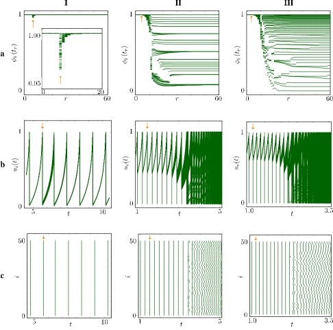
Figure 3.1. Desynchronization transition in a network with parameters $N=50$, $\varepsilon=0.0175$, $U=U_{b}$, $b=-3$, $R=R_{c}$ for different values of the partial reset strength: (I) $c=0.025<c_{\mathrm{cr}}^{(N)}$, (II) $c=0.5\in\left(c_{\mathrm{cr}}^{(N)},c_{\mathrm{cr}}^{(2)}\right)$ and (III) $c=0.7>c_{\mathrm{cr}}^{(2)}$. Plotted are (a) the phases $\phi_{i}\left(t_{r}\right)$ of all units at pulse generation times $t_{r}$ of the $r$-th spike of a reference unit (cf. return map (3.9)), (b) potential traces of all units and (c) the raster plots marking the times of pulse generation of each unit $i$. The network is started in the synchronous state and then a small perturbation is applied at a time indicated by arrows.

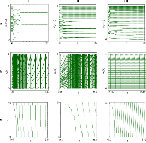
Figure 3.2. Same as in Fig. 3.1 but starting the dynamics form random initial phases distributed uniformly in the interval $[0,1)$. (IIIb) As the transient is similar to (IIb) a close up of the asymptotic asynchronous (splay) state is shown instead. In (c) the oscillator are labeled by increasing initial phases.

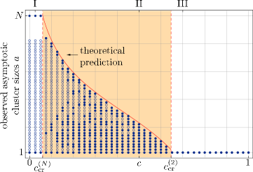
Figure 3.3. Sequential desynchronization transition in a network of $N=50$ units ($U=U_{b}$, $b=-3$, $\tilde{\varepsilon}=0.0175$). Asymptotic cluster sizes $a$ observed in the asymptotic network dynamics of $500$ simulations for each $c\in\left\{0,0.025,\dots,1\right\}$ starting from a perturbed synchronous state ($\bullet$, cf. fig. 3.1) or from other random phases distributed uniformly in $[0,1)$ ($\circ$ cf. fig. 3.2). The shaded area marks the sequential desynchronizing transition, the solid line shows the exact theoretical prediction (3.36) continuously interpolating the $N-1$ bifurcation points $c_{\mathrm{cr}}^{(a)}$, $a\in\left\{2,3,\dots,N\right\}$ above which clusters of size $a$ become unstable. The gap for clusters sizes $43<a<50$ at $0<c<c_{\mathrm{cr}}^{(2)}$ appears as cluster states involving these avalanche sizes do not exist according to lemma 7.

3.2. Strategy of the Analysis

We split up our analysis of the dynamics into two parts. First we assume that all avalanches are invariant, i.e. the given clusters do not decay into smaller sub-clusters. This assumption allows to group all oscillators firing in a single avalanche together into a single “meta-oscillator” with increased firing strength and an effective self interaction (cf. fig. 3.4). The analysis of a state $\Phi$ in homogeneous all-to-all network ($\varepsilon_{ij}=(1-\delta_{ij})\varepsilon$) of $N$ oscillators with avalanche sizes $a_{s}$, $s\in\left\{1,2,\dots,m\right\}$, $\sum_{s}a_{s}=N$ then reduces to analyzing a network of $m$ meta-oscillators with coupling strengths

(3.3) $$\varepsilon_{ij}=(1-\delta_{ij})\varepsilon_{i}+\delta_{ij}\varepsilon_{ii}$$

and $\varepsilon_{i}=a_{i}\varepsilon$, $\varepsilon_{ii}=(a_{i}-1)\varepsilon$.

In a second step we derive conditions under which an avalanche of a certain size will indeed not decay into smaller groups.

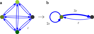
Figure 3.4. Network reduction method. (a) A network of $N=4$ oscillators producing an avalanche of three units as in Fig. 2.1 may be effectively reduced to (b) a smaller network of size $N=2$ with inhomogeneous coupling and self-interactions by grouping the oscillators involved in the avalanche to a single meta-oscillator. The effective network connectivity then has the form (3.3).

3.3. Notations: State Space, Firing and Return Map

A state of a network of $N$ pulse-coupled oscillators is completely specified by a phase vector

(3.4) $$\Phi=\left(\phi_{1},\phi_{2},\dots,\phi_{N}\right)\in S^{N}=\underbrace{S^{1}\times\dots\times S^{1}}_{N\>\text{times}}$$

where $\phi_{i}\in S^{1}=\mathbb{R}/\mathbb{Z}$ are the phases of the individual units. Since the time evolution in between avalanches is a pure phase shift (2.14) it is convenient to consider a Poincare section $\mathcal{S}$ of $S^{N}$ with states just before the firing of one or more oscillators, i.e.

(3.5) $$\mathcal{S}=\left\{\Phi\in S^{N}\>|\>\exists j\in\left\{1,\dots,N\right\},\>\phi_{j}=1\right\}\>.$$

It is convenient to relabel the oscillators after each avalanche such that $1=\phi_{1}\geq\phi_{2}\geq\dots\phi_{N-1}\geq\phi_{N}>0$. To specify the state of the network completely the permutation $\pi^{-1}$ used for relabeling of the oscillators is remembered. The largest phase $\phi_{1}=1$ thus belongs to the oscillator $i=\pi(1)$, the second largest $\phi_{2}$ to $i=\pi(2)$, etc., and the smallest $\phi_{N}$ to oscillator $i=\pi(N)$. Thus an equivalent description of the state space $\mathcal{S}$ is given by

(3.6) $$\mathcal{S}^{p}=\left\{\left(\left(\phi_{2},\dots,\phi_{N}\right),\pi\right)\in S^{N-1}\times S_{N}\>|\>1\geq\phi_{2}\geq\dots\phi_{N-1}\geq\phi_{N}\geq 0\right\}$$

Here $S_{N}$ is the group of all permutations of $N$ elements. We use the convention that all index labels $i$ are taken modulo the network size $N$, e.g. labels $i=j$ and $i=N+j$ denote the same oscillator.

The Poincare map of the network dynamics for the Poincare section $\mathcal{S}$ is the firing-map $\mathbf{K}$ that maps the state $\Phi\in\mathcal{S}$ of the network just before the $s$-th firing time $t_{s}$ of an avalanche to the state just before the next avalanche that occurs at time $t_{s+1}$:

(3.7) $$\mathbf{K}\left(\Phi\left(t_{s}^{-}\right)\right)=\Phi\left(t_{s+1}^{-}\right)\in\mathcal{S}$$

Having determined the next avalanche $\Theta$ from a state $\Phi\in\mathcal{S}$, the map $\mathbf{K}$ is a composition of the avalanche map (2.18) and a subsequent shift of all phases to a state in $\mathcal{S}$. Note that the firing map is fully determined by the pair $\left(\Theta,\sigma\right)$ which is a function of $\Phi$. We denote a phase shift of size $\sigma$ by

(3.8) $$S\left(\phi,\sigma\right):=S_{\sigma}\left(\phi\right):=\phi+\sigma$$

The equivalent firing map acting on the state space $\mathcal{S}^{p}$ is denoted by $\mathbf{K}^{p}$. For the phase part we write

$$\mathbf{K}_{\Phi}^{p}\left(\left(\psi_{2}^{(0)},\dots,\psi_{N}^{(0)}\right),\pi^{(0)}\right)=\left(\psi_{2}^{(1)},\dots,\psi_{N}^{(1)}\right)\,.$$

To track the network dynamics we consider a mapping of the state just before a fixed reference oscillator $k$ fires in an avalanche at time $t_{r}$ to the state just before this oscillator fires again at $t_{r+1}$:

(3.9) $$\mathbf{M}\left(\Phi\left(t_{r}^{-}\right)\right)=\Phi\left(t_{r+1}^{-}\right)$$

$\mathbf{M}$ is called the return-map and is the Poincaré map of the system on the section $\left\{\Phi\in\mathcal{S}\,|\,\phi_{k}=1\right\}$. Again the equivalent return map acting on $\mathcal{S}^{p}$ is denoted by $\mathbf{M}^{p}$. The number $m$ of avalanches occurring in the application of the return map is a function of the initial phase vector $\Phi=\Phi\left(t_{r}^{-}\right)$ and the return map $\mathbf{M}$ then is a composition of $m$ firing maps $\mathbf{K}$. Thus $\mathbf{M}$ is completely specified by an ordered firing sequence

(3.10) $$\mathcal{F}=\mathcal{F}\left(\Phi\right)=\left\{\left(\Theta_{s},\sigma_{s}\right)\right\}_{s=1}^{m}$$

where the pairs $\left(\Theta_{s},\sigma_{s}\right)$ specify the avalanche set $\Theta_{s}$ and subsequent shift $\sigma_{s}$ of the $s$-th firing map.

Given a firing sequence (3.10), we set $a_{s}=\left|\Theta_{s}\right|$ and in the case of homogenous networks with coupling (3.1), $\varepsilon_{s}=a_{s}\varepsilon$. A composition of shift and interaction maps is denoted as

(3.11) $$\bigodot_{s=1}^{m}\left(S_{\sigma_{s}}\circ H_{\varepsilon_{s}}\right)\left(\phi\right):=S_{\sigma_{m}}\circ H_{\varepsilon_{m}}\circ S_{\sigma_{m-1}}\circ H_{\varepsilon_{m-1}}...\circ S_{\sigma_{2}}\circ H_{\varepsilon_{2}}\circ S_{\sigma_{1}}\circ H_{\varepsilon_{1}}\left(\phi\right)$$

3.4. Existence and Stability of Asynchronous Periodic States in Meta-Oscillator Networks

Definition 5.

An asynchronous periodic state of a network of $N$ pulse-coupled oscillators is a state $\Phi\in\mathcal{S}$ which is invariant under the return map, i.e. $\mathbf{M}\left(\Phi\right)=\Phi$, and with avalanche sizes $a_{s}=1$, $s\in\left\{1,2,\dots,N\right\}$, i.e. each oscillator generates a pulse separately and does not receive supra-threshold input.

Initially assume that all clusters stay forward invariant, i.e. do not decay in to smaller sub-clusters during the network dynamics (cf. sec. 3.2) and thus consider networks of meta-oscillators with effective coupling matrix (3.3). A periodic cluster state in the original model thus becomes an periodic asynchronous state in the reduced effective meta-network. In the following we derive conditions for the existence of the asynchronous state and its stability in a meta-network.

Lemma 6.

Consider a network (2.17)-(2.18) of $N$ oscillators with pulse coupling matrix (3.3) and neuronal partial reset. Let $\Sigma=\left(\sigma_{1},\dots,\sigma_{N}\right)\in\mathbb{R}^{N}$ and define $\mathbf{L}:\mathbb{R}^{N}\times S^{1}\rightarrow\mathbb{R}^{N}$ by

$$\mathbf{L}_{i}(\Sigma,\phi):=\bigodot_{s=i+1}^{N+i-1}\left(S_{\sigma_{s}}\circ H_{\varepsilon_{s}}\right)\circ S_{\sigma_{i}}\circ J_{\varepsilon_{ii}}(\phi)$$

for $i\in\left\{1,2,\dots,N\right\}$. Then the asynchronous state exists if and only if there is a solution $\Sigma^{*}\in\mathbb{R}^{N}$ to the equation

(3.12) $$\mathbf{L}(\Sigma,1)=\left(1,1,\dots,1\right)$$

that satisfies $\sigma_{r}^{*}>0$ for all $r\in\left\{1,2,\dots,N\right\}$.

Proof.

Assume there is a solution $\Sigma^{*}$, $\sigma_{i}^{*}>0$. Set

$$\phi_{1}^{*}=1,\quad\quad\phi_{i}^{*}=\left(H_{\varepsilon_{1}}^{-1}\circ S_{\sigma_{1}^{*}}^{-1}\right)\circ\left(H_{\varepsilon_{2}}^{-1}\circ S_{\sigma_{2}^{*}}^{-1}\right)\circ\dots\circ\left(H_{\varepsilon_{i-1}}^{-1}\circ S_{\sigma_{i-1}^{*}}^{-1}\right)(1)$$

for $i\in\left\{2\dots,N\right\}$. Using that $\Sigma^{*}$ is a solution to (3.12) we have $\bigodot_{r=1}^{N-1}\left(S_{\sigma_{r}^{*}}\circ H_{\varepsilon_{r}}\right)\circ S_{\sigma_{N}^{*}}\circ J_{\varepsilon_{NN}}(1)=1$ and $\phi_{N}^{*}=S_{\sigma_{N}^{*}}\circ J_{\varepsilon_{NN}}(1)>0$ since $\sigma_{N}^{*}>0$. Further using $\varepsilon_{i}>0$ and $\sigma_{r}^{*}>0$ the phases are ordered according to $\phi_{1}^{*}=1>\phi_{2}^{*}>\dots>\phi_{N}^{*}>0$ and $\Phi^{*}=\left(\phi_{1}^{*},\phi_{2}^{*},\dots,\phi_{N}^{*}\right)\in\mathcal{S}$.

Starting from the state $\Phi^{*}$ the first pulse of oscillator $i=1$ results in potentials $u_{1}^{(1)}=R\left(\varepsilon_{11}\right)$, $u_{i}^{(1)}=U\left(\phi_{i}^{*}\right)+\varepsilon_{1}$, $i\in\left\{2,3,\dots,N\right\}$. Since $R\left(\varepsilon_{ii}\right)\leq\varepsilon_{ii}\leq\varepsilon_{i}<\varepsilon_{i}+U(\phi)$ for all $\phi>0$ and $H_{\varepsilon_{i}}(\phi)<H_{\varepsilon_{i}}(\psi)$ for $\phi<\psi$ we have $u_{1}^{(1)}<u_{N}^{(1)}<u_{N-1}^{(1)}<\dots<u_{2}^{(1)}$. Further

$$u_{2}^{(1)}=U\left(\phi_{2}^{*}\right)+\varepsilon_{1}=U\left(\left(H_{\varepsilon_{1}}^{-1}\circ S_{\sigma_{1}^{*}}^{-1}\right)(1)\right)+\varepsilon_{1}=U\left(1-\sigma_{1}^{*}\right)<1$$

as $\sigma_{1}^{*}>0$. Thus oscillator $i=1$ fires without triggering any further oscillators yielding an avalanche set $\Theta_{1}=$ $\left\{1\right\}$. In addition the oscillators have to be shifted by $\sigma_{1}^{*}$ to obtain $\phi_{2}=1$. Thus the first pair in the firing sequence is $\left(\left\{1\right\},\sigma_{1}^{*}\right)$. Applying the same arguments to the new phases $\Phi^{*(1)}=\mathbf{K}\left(\Phi^{*}\right)$ yields $\left(\left\{2\right\},\sigma_{2}^{*}\right)$ for the second pair. Repeating these steps $N$ times one obtains a firing sequence

$$\mathcal{F}\left(\Phi^{*}\right)=\left\{\left(\left\{r\right\},\sigma_{r}^{*}\right)\right\}_{r=1}^{N}$$

Thus

$$\mathbf{M}_{i}\left(\Phi^{*}\right) = \bigodot_{r=i+1}^{N}\left(S_{\sigma_{r}^{*}}\circ H_{\varepsilon_{r}}\right)\circ S_{\sigma_{i}^{*}}J_{\varepsilon_{ii}}\circ\bigodot_{r=1}^{i-1}\left(S_{\sigma_{r}^{*}}\circ H_{\varepsilon_{r}}\right)\left(\phi_{i}^{*}\right)$$

$$= \bigodot_{r=i+1}^{N}\left(S_{\sigma_{r}^{*}}\circ H_{\varepsilon_{r}}\right)\circ S_{\sigma_{i}^{*}}J_{\varepsilon_{ii}}(1)$$

$$= \left(H_{\varepsilon_{1}}^{-1}\circ S_{\sigma_{1}^{*}}^{-1}\right)\circ\left(H_{\varepsilon_{2}}^{-1}\circ S_{\sigma_{2}^{*}}^{-1}\right)\circ\dots\circ\left(H_{\varepsilon_{i-1}}^{-1}\circ S_{\sigma_{i-1}^{*}}^{-1}\right)(1)$$

$$= \phi_{i}^{*}$$

using (3.12) in the third row. Hence $\mathbf{M}\left(\Phi^{*}\right)=\Phi^{*}$ and the asynchronous state $\Phi^{*}$ is invariant under the return map.

Conversely an periodic asynchronous state yields a solution to (3.12), since by definition no oscillator receives supra-threshold input and thus there are a phase shifts $\sigma_{i}>0$ after each pulse generation of oscillators $i\in\left\{1,2,\dots,N\right\}$. Invariance of the periodic asynchronous state then shows that in fact $\Sigma=\left(\sigma_{1},\sigma_{2},\dots,\sigma_{N}\right)$ is a solution to (3.12). Hence there is no periodic asynchronous state if the solution does not exist. If there is a solution with $\sigma_{i}^{*}\leq 0$, let $s$ be the smallest index such that $\sigma_{s}^{*}\leq 0$. Starting in the state $\Phi^{*}$ the first firing of oscillator $i=s$ will cause oscillator $i=s+1$ to fire in the same avalanche since its potential at this point is given by

$$u_{s+1}^{(1)} = U\left[\bigodot_{r=1}^{s-1}\left(S_{\sigma_{r}^{*}}\circ H_{\varepsilon_{r}}\right)\left(\phi_{s+1}^{*}\right)\right]+\varepsilon_{s}$$

$$= U\left[H_{\varepsilon_{s}}^{-1}\circ S_{\sigma_{s}^{*}}^{-1}\left(1\right)\right]+\varepsilon_{s}=U\left(1-\sigma_{s}^{*}\right)\geq 1$$

i.e. $\left\{r,r+1\right\}\subset\Theta_{r}$ and the system is not in a periodic asynchronous state. ∎

Corollary 7.

In a network (2.17)-(2.18) of $N$ oscillators with homogeneous all-to-all coupling matrix (3.1) an asynchronous (splay) state exists.

Proof.

Let

$$L(\sigma):=\bigodot_{s=1}^{N-1}\left(S_{\sigma}\circ H_{\varepsilon}\right)\circ S_{\sigma}\circ J_{0}(1)$$

Now since $L(0)=U^{-1}\left(\varepsilon(N-1)\right)<1$ and $\frac{\partial}{\partial\sigma}L(\sigma)\geq 1$ the intermediate value theorem ensures the existence of a $\sigma^{*}>0$ satisfying $L\left(\sigma^{*}\right)=1$. $\Sigma^{*}=\left(\sigma^{*},\dots,\sigma^{*}\right)$ is a solution to (3.12). This result is independent of the partial reset $R$ as $\varepsilon_{ii}=0$ and no oscillator receives supra-threshold input in the asynchronous state. ∎

In Fig. 3.3 we observe no cluster states involving avalanches of size 43 to 49. This is precisely because 3.12 has no solutions when setting $\varepsilon_{i}=a_{i}\varepsilon$, $\varepsilon_{ii}=(a_{i}-1)\varepsilon$ for $a_{1}\in\left\{43,44,\dots,49\right\}$ and any further $0<a_{i}\in\mathbb{N}$, $i\geq 1$ and $m$ such that $\sum_{s=1}^{m}a_{s}=50$.

Note that lemma 7 holds for any rise function $U$. If there are $q$ different positive solutions to (3.12) there coexist $q$ different periodic asynchronous states. A convex $U$ ensures that the solution is unique because $\mathbf{L}\left(\Sigma,1\right)$ then becomes invertible for all $\Sigma\in\mathbb{R}^{N}$. Another consequence of convexity is that given the existence of an asynchronous state in a meta-oscillator network it is linearly stable as the following theorem shows:

Theorem 8.

Consider a network (2.17)-(2.18) of $N$ oscillators with pulse coupling matrix (3.3) and neuronal partial reset. If a periodic asynchronous state exist it is linearly stable.

Proof.

Existence of the asynchronous state $\left(\Phi^{*},\mathrm{id}\right)\in\mathcal{S}^{p}$ with $\Phi^{*}=\left(\phi_{2}^{*},\dots,\phi_{N}^{*}\right)$ implies invariance under the return map $\mathbf{M}^{p}$,

(3.13) $$\mathbf{M}^{p}\left(\Phi^{*},\mathrm{id}\right)=\left(\Phi^{*},\mathrm{id}\right)$$

For the intermediate states we set

$$\left(\Phi^{(s)},\mathrm{\pi^{(s)}}\right):=\left(\mathbf{K}^{p}\right)^{s}\left(\Phi^{*},\mathrm{id}\right)\quad s\in\left\{0,1,2,\dots,N\right\}$$

If oscillator $i$ generates a pulse all oscillators $j\neq i$ receive the same input $\varepsilon_{i}$ and oscillator $i$ receives an input $\varepsilon_{ii}\leq\varepsilon_{i}$. Hence, using $R(\zeta)\leq\zeta$, we find that the oscillators do not change their firing order and $\pi^{(s)}$ is a cyclic permutation to the left $\pi^{(s)}(i)=i-s$.

We show that the asynchronous state is linearly stable: Adding a perturbation $\Delta^{(0)}=\left(\delta_{1}^{(0)},...,\delta_{N-1}^{(0)}\right)$ to the asynchronous state such that initially the phases are given by

$$\Psi^{(0)}:=\left(\phi_{1}^{(0)},...,\phi_{N-1}^{(0)}\right)=\Phi^{*}+\Delta^{(0)}$$

We take the perturbation to be sufficiently small such that the oscillators still fire asynchronously, i.e. the avalanches are of size $a_{s}=1$ and the order of the events is preserved. In the following, terms of order $\mathcal{O}\left(\left(\Delta^{(0)}\right)^{2}\right)$ are neglected which we indicate by a dot above the equality sign ($\doteq$). After $s$ firing events the phases are

$$\Psi^{(s)}=\mathbf{K}_{\Phi}^{p}\left(\Psi^{(s-1)},\pi^{(s-1)}\right)\doteq\mathbf{K}_{\Phi}^{p}\left(\Phi^{(s-1)},\pi^{(r-1)}\right)+\Delta^{(s)}=\Phi^{(s)}+\Delta^{(s)}$$

where

$$\Delta^{(s)}=\mathbf{A}^{(s)}\Delta^{(s-1)}$$

is the phase perturbation before the next firing and $\mathbf{A}^{(s)}$ is the Jacobian matrix of $\mathbf{K}_{\Phi}^{p}$ at $\left(\Phi^{(s-1)},\pi^{(s-1)}\right)$

(3.14) $$A_{ij}^{(s)}=\frac{d\mathbf{K}_{i}^{p}}{d\phi_{j}}\left(\Phi^{(s-1)},\pi^{(s-1)}\right)\,.$$

Setting $\sigma=1-H\left(\psi_{2},\varepsilon_{\pi(1)}\right)$ the phase part of the firing-map for $N\geq 3$ is

(3.15) $$\boldsymbol{K}_{\Phi}^{p}\left(\Psi,\pi\right)=\left(\begin{array}[]{c}H\left(\psi_{3},\varepsilon_{\pi(1)}\right)+\sigma\\ H\left(\psi_{4},\varepsilon_{\pi(1)}\right)+\sigma\\ \dots\\ H\left(\psi_{N},\varepsilon_{\pi(1)}\right)+\sigma\\ J\left(1,\varepsilon_{\pi(1)\pi(1)}\right)+\sigma\end{array}\right)^{T}$$

Inserting (3.15) into (3.14) gives

(3.16) $$\mathbf{A}^{(s)}=\left(\begin{array}[]{ccccc}-a_{2}^{(s)}&a_{3}^{(s)}&0&\dots&0\\ -a_{2}^{(s)}&0&a_{4}^{(s)}&\ddots&\vdots\\ \vdots&\vdots&\ddots&\ddots&0\\ -a_{2}^{(s)}&0&\dots&0&a_{N}^{(s)}\\ -a_{2}^{(s)}&0&\dots&0&0\end{array}\right)$$

with

(3.17) $$a_{i}^{(s)}=\frac{d}{d\phi}H_{\varepsilon_{s}}\left(\phi_{i}^{(s-1)}\right)=\frac{U^{\prime}\left(\phi_{i}^{(s-1)}\right)}{U^{\prime}\left(H_{\varepsilon_{s}}\left(\phi_{i}^{(s-1)}\right)\right)}$$

Since $\varepsilon_{j}>0$ it follows that $H_{\varepsilon_{j}}\left(\phi\right)=U^{-1}\left(U(\phi)+\varepsilon_{j}\right)>\phi$. Thus $a_{i}^{(s)}<1$ since $U$ is convex. Also $U^{\prime}>0$ and hence

(3.18) $$0<a_{i}^{(s)}<1$$

Now the Eneström-Kakeya theorem (cf. appendix A and [24, 34, 4, 32]) applied to the matrix $\mathbf{A}^{(s)}$ shows that with these properties the spectral radius $\rho\left(\mathbf{A}^{(s)}\right)$ of $\mathbf{A}^{(s)}$ satisfies

$$\rho\left(\mathbf{A}^{(s)}\right)\leq r^{(s)}=\max_{i\in\left\{1,...,N-1\right\}}a_{i}^{(s)}<1$$

Thus

(3.19) $$\left\|\Delta^{(nN)}\right\|=\left\|\left(\prod_{r=1}^{N}\mathbf{A}^{(s)}\right)^{n}\Delta^{(0)}\right\|\leq\prod_{r=1}^{N}\rho\left(\mathbf{A}^{(s)}\right)^{n}\left\|\Delta^{(0)}\right\|\rightarrow 0\quad\quad\textrm{as }n\rightarrow\infty$$

and the asynchronous state is linearly stable. For $N=2$, $\rho\left(\mathbf{A}^{(s)}\right)=a_{2}<1$. ∎

This result is illustrated in Fig. 3.5: Due to the convexity of the rise function oscillators perturbed to larger (smaller) phases compared to the asynchronous state are less (more) advanced by input pulses pulling the perturbed phases back to the invariant asynchronous dynamics.

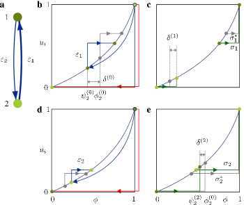
Figure 3.5. Stability of the asynchronous state. (a) Graph a network of $N=2$ oscillators with connectivity $\varepsilon_{ij}=\left(1-\delta_{ij}\right)\varepsilon_{j}$ with $0<\varepsilon_{2}<\varepsilon_{1}$. (b) Firing of oscillator $i=1$. For the oscillator $i=2$ with initial phase $\psi_{2}^{(0)}=\phi_{2}^{(0)}+\delta^{(0)}$ smaller than in the invariant asynchronous state $\phi_{2}^{(0)}$ (gray) the input advances the phase $\psi_{2}^{(0)}$ more in comparison with the advance of $\phi_{2}^{(0)}$ in the asynchronous state due to the convexity of the rise function. (c) After the interaction a subsequent shift completes the firing map $\mathbf{K}$. In total the derivation from the asynchronous state $\delta^{(1)}$ has become smaller. (d) Firing of oscillator $i=2$. Phases which are perturbed to larger values than the asynchronous state are less advanced by inputs due to convexity of the rise function, i.e. $H_{\varepsilon_{1}}\left(\psi_{2}^{(0)}\right)-\psi_{2}^{(0)}>H_{\varepsilon_{1}}\left(\phi_{2}^{(0)}\right)-\phi_{2}^{(0)}$. (d) In total the return map $\mathbf{M}$ decreases the phase perturbations $\left|\delta^{(2)}\right|<\left|\delta^{(0)}\right|$. These stabilizing dynamics of the asynchronous state due to the convexity of the rise function generalizes to larger networks as proven in theorem 8.

Combining corollary 7 and theorem 8 we obtain:

Corollary 9.

In a network (2.17)-(2.18) of $N$ oscillators with homogeneous all-to-all coupling matrix (3.1), neuronal partial reset $R$ and convex rise function $U$ the periodic asynchronous (splay) state exists and is linearly stable.

3.5. Impact of Partial Reset on Intra-Cluster Stability

In the state of synchronous firing all units in an all-to-all coupled network receive a supra-threshold input pulse of strength $\left(N-1\right)\varepsilon$ suggesting a rather strong influence of the partial reset $R$ onto the network dynamics. Indeed, as shown in Fig. 3.3 for the partial reset $R_{c}$ one observes a sequential destabilization of clusters when increasing the reset strength $c$. In this subsection we study this behavior analytically and explain the observed transition. The strategy is to focus on a single cluster and derive general conditions which ensure the stability of this cluster under the return map. As the return map depends on the firing sequence $\mathcal{F}$ only we give lower bounds below which cluster sizes are ensured to be stable and upper bounds above which cluster sizes are unstable. However, we find that for a special class of rise functions a full analytical treatment is possible.

Definition 10.

A firing sequence $\mathcal{F}$ is admissible if there is a state $\Phi\in\mathcal{S}$ which has firing sequence $\mathcal{F}=\mathcal{F}(\Phi)$. It is further called trigger invariant if for the oscillators $i\in\Theta_{1}^{(0)}=\left\{j\in\left\{1,2,\dots,N\right\}\,|\,\phi_{j}=1\right\}$ triggering the first avalanche of the state $\Phi=\left(\phi_{1},\dots,\phi_{N}\right)$ (cf. (2.9)) the return map satisfies $\mathbf{M}_{i}(\Phi)=1$. Thus for a trigger invariant firing sequence $\mathcal{F}$ with $m$ intermediate avalanches $\Theta_{1}^{(0)}\subset\Theta_{m+1}^{(0)}$. The set of all trigger invariant firing sequences is denoted by $\mathcal{T}$. The set of $\mathcal{F}\in\mathcal{T}$ with initial avalanche size $a_{1}=\left|\Theta_{1}\right|$ is denoted by $\mathcal{T}_{a_{1}}$.

Let us focus on a single avalanche of size $a_{1}$ in the network dynamics. To ensure that all units in this avalanche fire together again after the return map is applied all units in this avalanche which were triggered to fire by $a\in\left\{1,2,\dots,a_{1}-1\right\}$ preceding spikes i.e. with phases in

$$I_{a}^{T}=\left[U^{-1}\left(1-a\varepsilon\right),1\right]$$

have to be triggered again after applying the return map. Given a firing sequence $\mathcal{F}=\left\{\left(\varepsilon_{r},\sigma_{r}\right)\right\}_{r=1}^{m}$ the return map for oscillators $i\in\Theta_{1}$ in the first avalanche is given by

$$M_{\mathcal{F}}(\phi):=\bigodot_{r=2}^{m}\left(S_{\sigma_{r}}\circ H_{\varepsilon_{r}}\right)\circ S_{\sigma_{1}}\circ J_{\varepsilon_{1}}\left(\phi\right)$$

Hence the conditions

(3.20) $$\mathcal{M}_{\mathcal{F}}\left(I_{a}^{T}\right)\subset I_{a}^{T}$$

for all $a\in\left\{1,\dots,a_{1}-1\right\}$ and all admissible firing sequences $\mathcal{F}\in\mathcal{T}_{a_{1}}$ ensure a cluster of size $a_{1}$ to not split up under return.By finding the most synchronizing and most desynchronizing firing sequences (i.e. “best” and “worst case” firing sequences) $\mathcal{F}\in\mathcal{T}_{a_{1}}$ these conditions yield upper and lower bounds for stability of a cluster of size $a_{1}$ under the return map.

Lemma 11.

Consider a network (2.17)-(2.18) of $N$ oscillators with homogeneous all-to-all coupling matrix (3.1).

Set

$$w_{a}^{a_{1}}=\inf_{\mathcal{F}\in\mathcal{T}_{a_{1}}}M_{\mathcal{F}}\left(U^{-1}\left(1-a\varepsilon\right)\right)$$

and

$$b_{a}^{a_{1}}=\sup_{\mathcal{F}\in\mathcal{T}_{a_{1}}}M_{\mathcal{F}}\left(U^{-1}\left(1-a\varepsilon\right)\right)$$

Then the conditions

(3.21) $$w_{a}^{a_{1}}\geq U^{-1}\left(1-a\varepsilon\right)$$

for $a\in\left\{1,2,\dots,a_{1}-1\right\}$ are sufficient and

(3.22) $$b_{a}^{a_{1}}\geq U^{-1}\left(1-a\varepsilon\right)$$

are necessary for a cluster of size $a_{1}$ to be invariant under return.

Proof.

$\frac{\partial}{\partial\phi}M_{\mathcal{F}}(\phi)>0$ and thus conditions (3.20) are equivalent to $\mathcal{M}_{\mathcal{F}}\left(U^{-1}\left(1-a\varepsilon\right)\right)\geq U^{-1}\left(1-a\varepsilon\right)$ for $a\in\left\{1,2,\dots,a_{1}-1\right\}$ and all admissible $\mathcal{F}\in\mathcal{T}_{a_{1}}$. ∎

Finding the $w_{a}^{a_{1}}$ and $b_{a}^{a_{1}}$ for general $U$ and $R$ can be done numerically using optimization techniques. However, there are two classes of rise functions which allow further analytical investigation. Most of the commonly used rise functions, as e.g. the rise function of the LIF neuron or the conductance based LIF neuron fall into one of these classes (cf. Appendix B).

Two oscillators initially at phases $\phi$ and $\phi+\Delta\phi$ receiving a pulse of strength $\varepsilon$ will have a new phase difference

(3.23) $$\Delta H\left(\phi,\Delta\phi,\varepsilon\right):=H_{\varepsilon}\left(\phi+\Delta\phi\right)-H_{\varepsilon}\left(\phi\right)\;.$$

We denote the domain of $\Delta H$ as

$$\mathcal{D}:=\left\{\left(\phi,\Delta\phi,\varepsilon\right)\,|\,0\leq\varepsilon\leq 1,\,0\leq\phi\leq 1,\,0\leq\Delta\phi\leq U^{-1}\left(1-\varepsilon\right)-\phi\right\}\,.$$

Definition 12.

A rise function $U$ is increasing the change of phase differences (icpd) iff

(3.24) $$\frac{\partial}{\partial\phi}\Delta H\left(\phi,\Delta\phi,\varepsilon\right)\geq 0\quad\text{for all}\,\left(\phi,\Delta\phi,\varepsilon\right)\in\mathcal{D}\,.$$

Conversely, it is decreasing the change of phase differences (dcpd) iff

(3.25) $$\frac{\partial}{\partial\phi}\Delta H\left(\phi,\Delta\phi,\varepsilon\right)\leq 0\quad\text{for all}\,\left(\phi,\Delta\phi,\varepsilon\right)\in\mathcal{D}\>.$$

As shown in appendix B.2 the icpd (dcpd) property is related to the third derivative of $U$.

The following lemma allows to bound the change in phase differences if the rise function is icpd or dcpd:

Lemma 13.

Let $\varepsilon_{r}$, $\sigma_{r}\geq 0$, $r\in\left\{1,2,\dots,m\right\}$, $\varepsilon=\sum_{r=1}^{m}\varepsilon_{r}$, $\sigma_{l}\geq 0$. Choose a $\sigma_{u}\geq 0$ such that

$$\bigodot_{r=1}^{m}\left(S_{\sigma_{r}}\circ H_{\varepsilon_{r}}\right)\left(\phi\right)\leq H_{\varepsilon}\circ S_{\sigma_{u}}\left(\phi\right)\,.$$

and let $\psi\leq\phi$. Then for an icpd rise function $U$

(3.26) $$S_{\sigma_{l}}\circ H_{\varepsilon}\left(\phi\right)-S_{\sigma_{l}}\circ H_{\varepsilon}\left(\psi\right)\,\leq\,\bigodot_{r=1}^{m}\left(S_{\sigma_{r}}\circ H_{\varepsilon_{r}}\right)\left(\phi\right)-\bigodot_{r=1}^{m}\left(S_{\sigma_{r}}\circ H_{\varepsilon_{r}}\right)\left(\psi\right)\,\leq\,H_{\varepsilon}\circ S_{\sigma_{u}}\left(\phi\right)-H_{\varepsilon}\circ S_{\sigma_{u}}\left(\psi\right)$$

If $U$ is dcpd then

(3.27) $$S_{\sigma_{l}}\circ H_{\varepsilon}\left(\phi\right)-S_{\sigma_{l}}\circ H_{\varepsilon}\left(\psi\right)\geq\bigodot_{r=1}^{m}\left(S_{\sigma_{r}}\circ H_{\varepsilon_{r}}\right)\left(\phi\right)-\bigodot_{r=1}^{m}\left(S_{\sigma_{r}}\circ H_{\varepsilon_{r}}\right)\left(\psi\right)\geq H_{\varepsilon}\circ S_{\sigma_{u}}\left(\phi\right)-H_{\varepsilon}\circ S_{\sigma_{u}}\left(\psi\right)$$

Proof.

Consider icpd rise functions first: To show the first inequality of eq. (3.26) we use induction on $m$. The statement is clearly true for $m=1$. Assume it is true for $m\geq 1$ then

$$S_{\sigma_{l}}\circ H_{\varepsilon}\left(\phi\right)-S_{\sigma_{l}}\circ H_{\varepsilon}\left(\psi\right)=H_{\varepsilon_{m+1}}\circ H_{\varepsilon-\varepsilon_{m+1}}\left(\phi\right)-H_{\varepsilon_{m+1}}\circ H_{\varepsilon-\varepsilon_{m+1}}\left(\psi\right)$$

$$= \Delta H\left(H_{\varepsilon-\varepsilon_{m+1}}\left(\psi\right),H_{\varepsilon-\varepsilon_{m+1}}\left(\phi\right)-H_{\varepsilon-\varepsilon_{m+1}}\left(\psi\right),\varepsilon_{m+1}\right)$$

$$\leq \Delta H\left(H_{\varepsilon-\varepsilon_{m+1}}\left(\psi\right),\bigodot_{r=1}^{m}\left(S_{\sigma_{r}}\circ H_{\varepsilon_{r}}\right)\left(\phi\right)-\bigodot_{r=1}^{m}\left(S_{\sigma_{r}}\circ H_{\varepsilon_{r}}\right)\left(\psi\right),\varepsilon_{m+1}\right)$$

$$\leq \Delta H\left(\bigodot_{r=1}^{m}\left(S_{\sigma_{r}}\circ H_{\varepsilon_{r}}\right)\left(\psi\right),\bigodot_{r=1}^{m}\left(S_{\sigma_{r}}\circ H_{\varepsilon_{r}}\right)\left(\phi\right)-\bigodot_{r=1}^{m}\left(S_{\sigma_{r}}\circ H_{\varepsilon_{r}}\right)\left(\psi\right),\varepsilon_{m+1}\right)$$

$$= \bigodot_{r=1}^{m+1}\left(S_{\sigma_{r}}\circ H_{\varepsilon_{r}}\right)\left(\phi\right)-\bigodot_{r=1}^{m+1}\left(S_{\sigma_{r}}\circ H_{\varepsilon_{r}}\right)\left(\psi\right)$$

where we used the induction hypothesis and $\frac{\partial}{\partial\Delta\phi}\Delta H>0$ (cf. (3.23)) in the third, and in the fourth again the icpd property and the fact that $H_{\varepsilon-\varepsilon_{m+1}}\left(\psi\right)\leq\bigodot_{r=1}^{m}\left(S_{\sigma_{r}}\circ H_{\varepsilon_{r}}\right)$ if $\sum_{r=1}^{m+1}\varepsilon_{r}=\varepsilon$, $\sigma_{i}\geq 0$. Substituting $\leq$ with $\geq$ we obtain the result for dcpd rise functions.

For the second inequality we also use induction over $m$. The statement is trivially true for $m=1$. Let it be true for $m\geq 1$ and let $\sigma_{u}\geq 0$ such that $\bigodot_{r=1}^{m+1}\left(S_{\sigma_{r}}\circ H_{\varepsilon_{r}}\right)\left(\phi\right)\leq H_{\varepsilon}\circ S_{\sigma_{u}}\left(\phi\right)$. Then

$$H_{\varepsilon}\circ S_{\sigma_{u}}\left(\phi\right)-H_{\varepsilon} \circ S_{\sigma_{u}}\left(\psi\right)=H_{\varepsilon_{m+1}}\circ H_{\varepsilon-\varepsilon_{m+1}}\circ S_{\sigma_{u}}\left(\phi\right)-H_{\varepsilon_{m+1}}\circ H_{\varepsilon-\varepsilon_{m+1}}\circ S_{\sigma_{u}}\left(\psi\right)$$

$$=\Delta H\left(H_{\varepsilon-\varepsilon_{m+1}}\circ S_{\sigma_{u}}\left(\psi\right),H_{\varepsilon-\varepsilon_{m+1}}\circ S_{\sigma_{u}}\left(\phi\right)-H_{\varepsilon-\varepsilon_{m+1}}\circ S_{\sigma_{u}}\left(\psi\right),\varepsilon_{m+1}\right)$$

$$\geq\Delta H\left(H_{\varepsilon-\varepsilon_{m+1}}\circ S_{\sigma_{u}}\left(\psi\right),\bigodot_{r=1}^{m}\left(S_{\sigma_{r}}\circ H_{\varepsilon_{r}}\right)\left(\phi\right)-\bigodot_{r=1}^{m}\left(S_{\sigma_{r}}\circ H_{\varepsilon_{r}}\right)\left(\psi\right),\varepsilon_{m+1}\right)$$

$$\geq\Delta H\left(\bigodot_{r=1}^{m}\left(S_{\sigma_{r}}\circ H_{\varepsilon_{r}}\right)\left(\psi\right),\bigodot_{r=1}^{m}\left(S_{\sigma_{r}}\circ H_{\varepsilon_{r}}\right)\left(\phi\right)-\bigodot_{r=1}^{m}\left(S_{\sigma_{r}}\circ H_{\varepsilon_{r}}\right)\left(\psi\right),\varepsilon_{m+1}\right)$$

$$=\bigodot_{r=1}^{m+1}\left(S_{\sigma_{r}}\circ H_{\varepsilon_{r}}\right)\left(\phi\right)-\bigodot_{r=1}^{m+1}\left(S_{\sigma_{r}}\circ H_{\varepsilon_{r}}\right)\left(\psi\right)$$

where in the third row we used the implication

(3.28) $$\bigodot_{s=1}^{m+1}\left(S_{\sigma_{s}}\circ H_{\varepsilon_{s}}\right)\left(\phi\right)\leq H_{\varepsilon}\circ S_{\sigma_{u}}\left(\phi\right)\,\Rightarrow\,\bigodot_{s=1}^{m}\left(S_{\sigma_{s}}\circ H_{\varepsilon_{s}}\right)\left(\phi\right)\leq H_{\varepsilon-\varepsilon_{m+1}}\circ S_{\sigma_{u}}\left(\phi\right)$$

to apply the induction hypothesis. In the fourth row we again used $\frac{\partial}{\partial\Delta\phi}\Delta H>0$, eq. (3.28) and the icpd property. Substituting $\geq$ with $\leq$ we obtain the result for dcpd rise functions. ∎

This result is illustrated in Fig. 3.6 (a-c) for icpd rise functions.

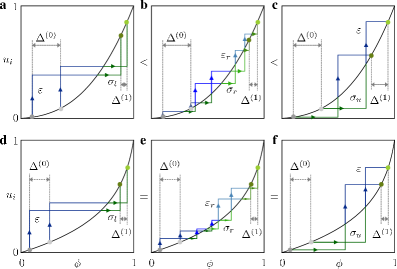
Figure 3.6. Rise functions with increasing change (icpd) and no change of phase differences. (a-c) Icpd rise function. An initial phase difference $\Delta^{(0)}$ changes to $\Delta^{(1)}$ after applying a combination of interaction maps $H_{\varepsilon_{r}}$ (blue) of total strength $\varepsilon=\sum_{r=1}^{m}\varepsilon_{r}$ and shifts $S_{\sigma_{r}}$ (green) such that the final maximal phase values are identical. (a) For icpd rise functions the difference $\Delta^{(1)}$ is the smallest when the interaction is applied in total before the shifts, i.e. $H_{\varepsilon}\circ S_{\sigma_{l}}$ and (c) largest when applied after the shifts $S_{\sigma_{u}}\circ H_{\varepsilon}$. (b) All other maps $\bigodot_{s=1}^{m}\left(H_{\varepsilon_{s}}\circ S_{\sigma_{s}}\right)$ produce phase differences which lie in between these extremal values (cf. lemma 13). (d-f) The rise function $U_{b}$ is icpd and dcpd, i.e. the phase difference $\Delta\phi^{(1)}$ is independent of the order in which the interactions and shifts are applied.

The next theorem allows to determine bounds on the network parameters in order to ensure invariance or decay of avalanches under return:

Theorem 14.

Consider a homogenous excitatory all-to-all network of $N$ pulse-coupled oscillators evolving according to (2.17)-(2.18) with neuronal partial reset $R$.

For icdp rise functions $U$ the conditions

(3.29) $$U^{-1}\left(R\left((a_{1}-1)\varepsilon\right)\right)-U^{-1}\left(R\left((a_{1}-1)\varepsilon-a\varepsilon\right)\right)\leq U^{-1}\left(1-(N-a_{1})\varepsilon\right)-U^{-1}\left(1-(N-a_{1})\varepsilon-a\varepsilon\right)$$

for all $a\in\left\{1,2,\dots,a_{1}-1\right\}$ are sufficient to ensure the invariance of an $a_{1}$-avalanche under return. Necessary conditions are

(3.30) $$U^{-1}\left(R\left((a_{1}-1)\varepsilon\right)+(N-a_{1})\varepsilon\right)-U^{-1}\left(R\left((a_{1}-1)\varepsilon-a\varepsilon\right)+(N-a_{1})\varepsilon\right)\leq 1-U^{-1}\left(1-a\varepsilon\right)\>.$$

Likewise for dcpd rise functions $U$ sufficient conditions are (3.30) and necessary conditions (3.29) for an $a_{1}$-avalanche to not split up under return.

Proof.

Using lemma 13 we find for an icpd rise function and $\mathcal{F}\in\mathcal{T}_{a_{1}}$

$$M_{\mathcal{F}}(1)-M_{\mathcal{F}}\left(U^{-1}\left(1-a\varepsilon\right)\right) = \bigodot_{r=2}^{m}\left(S_{\sigma_{r}}\circ H_{\varepsilon_{r}}\right)\left(S_{\sigma_{1}}\circ J_{\varepsilon_{1}}\left(1\right)\right)-\bigodot_{r=2}^{m}\left(S_{\sigma_{r}}\circ H_{\varepsilon_{r}}\right)\left(S_{\sigma_{1}}\circ J_{\varepsilon_{1}}\left(U^{-1}\left(1-a\varepsilon\right)\right)\right)$$

$$\leq H_{\left(N-a_{1}\right)\varepsilon}\circ S_{\sigma_{u}}\circ J_{\varepsilon_{1}}\left(1\right)-H_{\left(N-a_{1}\right)\varepsilon}\circ S_{\sigma_{u}}\circ J_{\varepsilon_{1}}\left(U^{-1}\left(1-a\varepsilon\right)\right)$$

$$= 1-H_{\left(N-a_{1}\right)\varepsilon}\circ S_{\sigma}\circ J_{\varepsilon_{1}}\left(U^{-1}\left(1-a\varepsilon\right)\right)$$

with

(3.31) $$\sigma_{u}=U^{-1}\left(1-\left(N-a_{1}\right)\varepsilon\right)-U^{-1}\left(R\left(a_{1}-1\right)\varepsilon\right)$$

and thus

$$w_{a}^{a_{1}}=H_{\left(N-a_{1}\right)\varepsilon}\circ S_{\sigma_{u}}\circ J_{\varepsilon_{1}}\left(U^{-1}\left(1-a\varepsilon\right)\right)$$

in (3.21) yielding conditions (3.29). Similarly we find

$$b_{a}^{a_{1}}=1-H_{\left(N-a_{1}\right)\varepsilon}\circ J_{\varepsilon_{1}}\left(1\right)+H_{\left(N-a_{1}\right)\varepsilon}\circ J_{\varepsilon_{1}}\left(U^{-1}\left(1-a\varepsilon\right)\right)$$

which yields the necessary conditions (3.30). For dcdp rise functions the expressions for $w_{a}^{a_{1}}$ and $b_{a}^{a_{1}}$ are interchanged. ∎

Proposition 15.

In a homogeneous all-to-all coupled network of $N$ neural oscillators evolving according to (2.17)-(2.18) with neuronal partial reset $R$ and dcdp rise function $U$ the condition

(3.32) $$R^{\prime}(\zeta)>\frac{U^{\prime}\left(U^{-1}\left(R(\zeta)\right)\right)}{U^{\prime}\left(U^{-1}\left(1-(N-1)\varepsilon+\zeta\right)\right)}\quad\text{for all}\>(a_{1}-2)\varepsilon\leq\zeta\leq(a_{1}-1)\varepsilon$$

is sufficient to ensure non-invariance of an $a_{1}$-cluster under return.

Proof.

Using lemma 13 for a given firing sequence $\mathcal{F}=\left\{\left(a_{s}\varepsilon,\sigma_{s}\right)\right\}_{s=1}^{m}$ we estimate

(3.33) $$1-H_{\left(N-a_{1}\right)\varepsilon}\circ S_{\sigma_{u}}\circ J_{\varepsilon_{1}}\left(1-\Delta\phi\right)\leq 1-M_{\mathcal{F}}\left(1-\Delta\phi\right)\leq 1-S_{\sigma_{l}}\circ H_{\left(N-a_{1}\right)\varepsilon}\circ J_{\varepsilon_{1}}\left(1-\Delta\phi\right)$$

with $\sigma_{u}$ as in (3.31) and $\sigma_{l}=1-H_{\left(N-a_{1}\right)\varepsilon}\left(J_{a_{1}\varepsilon}(1)\right)$. In general a $a_{1}$-cluster is triggered by a single oscillator and thus if

(3.34) $$1-H_{\left(N-a_{1}\right)\varepsilon}\circ S_{\sigma_{u}}\circ J_{a_{1}}\left(1-\Delta\phi\right)>\Delta\phi$$

for all $0<\Delta\phi\leq 1-U^{-1}\left(1-\varepsilon\right)$, we have $1-M_{\mathcal{F}}\left(1-\Delta\phi\right)>\Delta\phi$ which implies that after a finite number of iterations of the return map the firing of the first oscillator does not trigger the avalanche any more. Setting $\zeta=U\left(1-\Delta\phi\right)+(a_{1}-1)\varepsilon-1$ condition (3.34) is equivalent to

(3.35) $$U^{-1}\left(R\left((a_{1}-1)\varepsilon\right)\right)-U^{-1}\left(R\left(\zeta\right)\right)>U^{-1}\left(1-(N-a)\varepsilon\right)-U^{-1}\left(1-(N-1)\varepsilon+\zeta\right)$$

for all $(a_{1}-2)\varepsilon\leq\zeta<(a_{1}-1)\varepsilon$. For $\zeta=(a_{1}-1)\varepsilon$ both sides in (3.35) are equal and the condition (3.32) thus ensures (3.35) to hold for all $(a_{1}-2)\varepsilon\leq\zeta<(a_{1}-1)\varepsilon$. ∎

Note that for convex $U$ and neuronal $R$ the right hand side of inequality (3.32) is smaller than one and thus a sufficient condition for $a_{1}$-avalanches to split up after a finite number of applications of the return map is

$$R^{\prime}(\zeta)\geq 1\quad\text{for all }\,\zeta\in\left[(a_{1}-2)\varepsilon,(a_{1}-1)\varepsilon\right]$$

In particular for a partial reset $R_{c=1}(\zeta)=\zeta$ all avalanches become unstable under the return map and thus by corollary 9 only the asynchronous state remains stable for all convex dcpd $U$ and $c=1$.

We used theorem 8 and proposition 15 to determine for a convex LIF rise function $U_{\mathrm{LIF}}^{\mathrm{CB}}$ (cf. B.5 eq. (B.7)) and linear partial reset $R_{c}$ the regime where avalanches of different sizes become unstable under return. The most strict condition in (3.29) is for $a=1$ which yields an implicit equation for the lower bounds on the critical $c$ values below which the invariance of $a_{1}$-avalanches is ensured. The upper bound is obtained by (3.30) using $a=1$ and is very close to the bound given in proposition 15. The bounds are plotted in fig. 3.7 and are in good agreement with the numerical data.

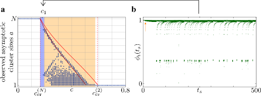
Figure 3.7. Sequential desynchronization in a network ($N=100$) with icpd rise function $U_{\mathrm{LIF}}^{\mathrm{CB}}$ ($E_{\mathrm{eq}}=1.1$, $E_{\mathrm{syn}}=3$) and linear partial reset $R_{c}$. (a) Observed cluster sizes of periodic states after a time $t=10000$. For each $c$ value $100$ simulations were started in the synchronous state with a small perturbation added. The upper line shows the bounds on $a$ obtained from (3.30) in theorem 14 above which $a$-clusters are unstable. The lower line is the bound obtained via (3.29) below which $a$-clusters are ensured to be stable. The shaded area marks the transition region where states other than the synchronous an asynchronous state are observed. In the blue region we find no periodic asymptotic dynamics. The dashed lines show the theoretical bounds for the transition region. (b) Aperiodic dynamics for $c_{1}=0.18$.

Near the lower transition point $c_{\mathrm{crit}}^{(N)}$ the system shows aperiodic behavior when starting close to the synchronous state. A possible explanation for this dynamics is the competition of two counteracting mechanisms: (i) Large avalanches become unstable under return and thus tend to desynchronize the phases which results in a split of the avalanche into smaller stable avalanches. (ii) The solution to equation (3.12) for these asynchronously firing smaller clusters involves $\sigma_{r}^{*}\leq 0$, i.e. the smaller avalanches tend to absorb each other and resynchronize the system yielding again larger unstable avalanches. Note that here irregular dynamics arise via a mechanism different form as for example network heterogeneity [15] or using excitatory and inhibitory interactions [67].

3.6. Extensive Sequence of Desynchronizing Bifurcations – A Solvable Example

Figure 3.6 (d-f) illustrates that the rise function $U_{b}$ is both icpd and dcpd. In fact,

$$\Delta H_{b}\left(\phi,\Delta\phi,\varepsilon\right):=H_{b}\left(\phi+\Delta\phi,\varepsilon\right)-H_{b}\left(\phi,\varepsilon\right)=\Delta\phi e^{b\varepsilon}$$

is independent of $\phi$ and hence

$$\frac{\partial}{\partial\phi}\Delta H_{b}\left(\phi,\Delta\phi,\varepsilon\right)=0\>.$$

Thus for $U_{b}$ equality holds in (3.26) and the ”best”- and ”worst-case” return maps become identical. This property allows to obtain exact analytical results.

Proposition 16.

Consider a homogenous excitatory all-to-all network of $N$ pulse-coupled oscillators evolving according to (2.17)-(2.18) with convex rise function $U_{b}$ ($b<0$) and neuronal partial reset $R_{c}$.

Then for each $2\leq a\leq N$ there exist a critical reset strength $c_{\mathrm{cr}}^{(a)}$ such that for all $c>c_{\mathrm{cr}}^{(a)}$ avalanches of size greater or equal to $a$ are unstable under return and avalanches of size smaller than $a$ are stable. For $c\leq c_{\mathrm{cr}}^{(N)}$ all avalanches are stable under return. The critical reset strengths are determined from the equation

(3.36) $$e^{b\left(1-\left[(N-a)+c_{\mathrm{cr}}^{(a)}(a-1)\right]\varepsilon\right)}=\frac{\left(e^{-bc_{\mathrm{cr}}^{(a)}\varepsilon}-1\right)}{\left(e^{-b\varepsilon}-1\right)}$$

and satisfy $0<c_{\mathrm{cr}}^{(N)}<c_{\mathrm{cr}}^{(N-1)}<\dots<c_{\mathrm{cr}}^{(2)}<1$.

Proof.

Since $U_{b}$ is icpd and dcpd, equality holds in (3.33), i.e. for $\mathcal{F}\in\mathcal{T}_{a_{1}}$

(3.37) $$\Delta M_{\mathcal{F}}\left(\Delta\phi\right):=1-M_{\mathcal{F}}\left(1-\Delta\phi\right) = 1-S_{\sigma_{l}}\circ H_{\left(N-a_{1}\right)\varepsilon}\circ J_{a_{1}\varepsilon}\left(1-\Delta\phi\right)$$

Thus the return map for the phase differences only depends on the avalanche size $a_{1}$ and is independent of the precise form of the other avalanches $a_{i}$, $i>1$ and intermediate shifts $\sigma_{i}$. Explicitly

$$\Delta M_{\mathcal{F}}\left(\Delta\phi\right)=\frac{e^{b\varepsilon\left(N-a_{1}+c(a_{1}-1)\right)}}{1-e^{b}}\left(e^{-bc}\left(e^{b}+\left(1-e^{b}\right)\Delta\phi\right)^{c}-1\right)$$

for all $\mathcal{F}\in\mathcal{T}_{a_{1}}$. A straight forward calculation shows that $\Delta M_{\mathcal{F}}$ has the properties

(3.38) $$\Delta M_{\mathcal{F}}\left(0\right)=0\quad,\quad\frac{d}{d\Delta\phi}\Delta M_{\mathcal{F}}\left(\Delta\phi\right)\geq 0\quad\textrm{and}\quad\frac{d^{2}}{d\Delta\phi^{2}}\Delta M_{\mathcal{F}}\left(\Delta\phi\right)\leq 0$$

Thus if the condition

(3.39) $$\Delta M_{\mathrm{\mathcal{F}}}\left(1-U^{-1}\left(1-\varepsilon\right)\right)\leq 1-U^{-1}\left(1-\varepsilon\right)$$

is met all other conditions for $1\leq a<a_{1}$ in (3.29) are also satisfied. On the other hand almost all perturbations will cause the avalanche to be triggered by a single oscillator. Thus if condition (3.39) is not satisfied, i.e. $\Delta M_{\mathcal{F}}\left(\Delta\phi\right)>\Delta\phi$ for all $\Delta\phi\geq U^{-1}\left(1-\varepsilon\right)-1$ the avalanche will split up after a finite number of iterations of the return map. Thus (3.39) is a necessary and sufficient condition for stability of an $a$-cluster under the return map. We are interested in the critical strengths $c_{\mathrm{crit}}^{(a)}$ for which an $a$-cluster becomes unstable and hence we use equality in (3.39) and basic algebra to obtain the implicit expressions (3.36) for the $c_{\mathrm{cr}}^{(a)}$.

Since we have assumed $\left(N-1\right)\varepsilon<1$, $b<0$ and $c\in\left[0,1\right]$ we see that the left hand side of (3.36) lies in the interval $\left(0,1\right)$ and decreases monotonically with increasing $c$. The right hand side is $0$ for $c=0$ and increases monotonically with $c$ until it becomes $1$ for $c=1$. Thus by continuity for all $2\leq a\leq N$ there always exist a solution $0<c_{\mathrm{cr}}^{(a)}<1$ to this equation. Note that the special case $a=2$ is explicitly solvable for $c_{\mathrm{cr}}^{(2)}$ and yields

(3.40) $$c_{\mathrm{cr}}^{(2)}=\frac{1}{b\varepsilon}\log\left(1+e^{-b(N-2)\varepsilon+b}\left(1-e^{-b\varepsilon}\right)\right)$$

For fixed $0\leq c<1$ the left hand side of (3.36) is strict monotonically decreasing as $a$ increases whereas the left hand side is independent of $a$, thus $0<c_{\mathrm{cr}}^{(N)}<c_{\mathrm{cr}}^{(N-1)}<\dots<c_{\mathrm{cr}}^{(2)}<1$. ∎

The theoretical prediction (3.36) for the desynchronization transition is plotted in Fig. 3.3 and is in excellent agreement with the numerically observed transition.

Remark 17.

Note that (3.36) involves all relevant network parameter. In particular, by choosing $b\rightarrow-\infty$ equation (3.40) shows that $c_{\mathrm{cr}}^{(2)}$ can be made arbitrarily small. This implies that the entire sequence of desynchronizing bifurcations may occur over an arbitrary small interval $\left[c_{\mathrm{cr}}^{(N)},c_{\mathrm{cr}}^{(2)}\right]$.

Remark 18.

We also remark that the number of bifurcation points in this sequence is $N-1$. At each bifurcation point $c_{\mathrm{cr}}^{(a)}$ all periodic states with at least one cluster of size $a$ and all other cluster sizes less or equal to $a$, i.e. an extensive combinatorial number of states, becomes unstable simultaneously.

The mechanism underlying the desynchronization transition are opposing synchronization and desynchronization dynamics in the network as illustrated in Fig. 3.8: Due to the convexity of the rise function (a) sub-threshold inputs are always synchronizing and stabilize the avalanche, whereas depending on the strength of the partial reset supra-threshold inputs in an avalanche can either (b) synchronize or (c) desynchronize the phases. Thus for a weak partial reset (e.g. $R_{c}$ with $c\approx 0$) states with large avalanches are stable. When the partial reset is stronger it desynchronizes the cluster and, depending on the avalanche size, it may outweigh the synchronization effect due to sub-threshold inputs. Larger avalanches receive less synchronizing sub-threshold input from other oscillators and simultaneously produce a larger supra-threshold input than smaller ones. Thus they lose invariance under return first when increasing the partial reset strength.

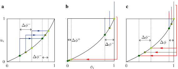
Figure 3.8. Synchronization and Desynchronization of avalanches in networks with convex rise function and partial reset. (a) Sub-threshold inputs synchronize the oscillators. The phase difference of a cluster before pulse reception $\Delta\phi^{+}$ is decreased to $\Delta\phi^{-}$ afterwards, i.e. $\Delta\phi^{+}<\Delta\phi^{-}$. (a) Weak partial reset (e.g. $c\approx 0$ for $R_{c}$) synchronize phase differences: $\Delta\phi^{+}<\Delta\phi^{-}$. (b) Due to the convexity of the rise function a strong partial reset ($c\approx 1$) expands the phase differences $\Delta\phi^{+}>\Delta\phi^{-}$. Clusters lose stability if mechanism in (c) becomes dominant over the stabilizing effect (a).

4. Robustness of the Desynchronization Transition

The desynchronization transition is robust against structural perturbations in the coupling matrix and the rise function $U$.

4.1. Coupling Strength Inhomogeneity

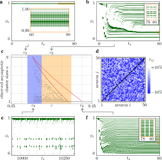
Figure 4.1. Sequential desynchronization transition in an inhomogeneous network. Shown are the dynamics of a network of $N=50$ units with convex rise-function $U_{\mathrm{LIF}}^{\mathrm{CB}}$ ($E_{\mathrm{eq}}=1.1$ and $E_{\mathrm{syn}}=3$) and linear partial reset $R_{c}$. (d) coupling strengths are drawn from a random uniform distribution from $\varepsilon_{ij}\in\left[0.009,0.011\right]$ excluding self-coupling ($\varepsilon_{ii}=0$). Simulations are initialized in a perturbed synchronous state. (a) Synchronous firing for $c_{1}=0.12$. Inset: Phase are not synchronized due to the coupling inhomogeneity. (b) For $c_{2}=0.19$ the synchronous state becomes unstable and smaller avalanches are observed in the asymptotic dynamics Inset: As in the synchronous state phases of units in a single avalanche are not phase synchronized. (e) For $c_{3}=0.16$ we do observe aperiodic firing until $t=15000$. (f) For $c_{4}=0.4$ asynchronous firing is observed in the asymptotic dynamics. Inset: Spacings of the phases are irregular due to the network heterogeneity. (c) Asymptotic cluster sizes of periodic states for different $c$ values starting from $100$ different perturbed synchronous states. The lines show the lower and upper estimates for the transition obtained from theorem 14 assuming a homogeneous network with coupling strength $\varepsilon=0.01$. The shaded blue area indicates that states with aperiodic dynamics until $t=15000$ are observed.

The desynchronization transition is robust against perturbations in the coupling matrix $\varepsilon_{ij}$. Our numerical experiments show that the transition is also observed when using coupling strengths from a uniform distribution on an interval $[\varepsilon_{\mathrm{min}},\varepsilon_{\mathrm{max}}]$ for a interval length $\Delta\varepsilon=\varepsilon_{\mathrm{max}}-\mathrm{\varepsilon_{min}}$ as large as $20\%$ of the average coupling strength $\bar{\varepsilon}=\left(\varepsilon_{\mathrm{max}}-\mathrm{\varepsilon_{min}}\right)/2$ (cf. fig. 4.1). When $\Delta\varepsilon$ becomes larger usually complex spike patterns and non-periodic states are observed.

In inhomogeneous networks sub-threshold inputs of different strengths desynchronize units initially at the same phase. Thus coupling inhomogeneity destabilizes clusters of a given size $a$. In fact, already the lower bound $c_{\mathrm{crit}}^{(a)}$ obtained for homogeneous networks via theorem 14 using the coupling strength $\bar{\varepsilon}$ over-estimates the stability of the clusters as shown in fig. 4.1. The regime where we observe aperiodic dynamics becomes larger in comparison to homogeneous networks with the same average coupling strength (e.g. compare fig. 4.1 and fig. 3.7). This is due to cluster states in the homogeneous network with asymptotic phases of the clusters which are close to an absorption (i.e. there are $\sigma_{i}^{*}\approx 0$ for some $i$). A perturbation in the coupling now enables the absorption and the restless competition between desynchronization and synchronization (cf. sec. 3.5) induces the aperiodic dynamics.

Another effect of inhomogeneous coupling is that units synchronized to fire together in clusters are not phase synchronized (cf. insets in fig. 4.1) in the asymptotic dynamics. Also intra-cluster phases of equally sized clusters and in particular of the asynchronous state show irregular spacings.

4.1.1. Sigmoidal Rise Functions

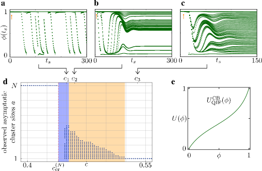
Figure 4.2. Sequential desynchronization transition in networks of neural oscillators with a sigmoidal rise function. Shown are the dynamics of a homogeneous network ($N=100$, $\varepsilon=0.002$) with linear partial reset $R_{c}$ and (e) sigmoidal rise function $U_{\mathrm{LIF}}^{\mathrm{CB}}$ ($E_{\mathrm{syn}}=2$, $\alpha=-1$, $\beta=1$). Starting with synchrony and inducing a small perturbation (arrow) the network shows (a) aperiodic dynamics for $c=c_{1}=0.45$, (b) clustering for $c=c_{2}=0.46$ and (c) asynchronous dynamics for $c=c_{3}=0.54$. Note the oscillations of the phase which do not appear for purely convex rise functions (cf. fig. 3.7). (d) Cluster sizes of periodic states observed in the dynamics at $t=5000$ starting from $200$ perturbed synchronous states for each value of $c$. Shaded area marks the transition region with states other than solely synchronous or asynchronous. The blue shaded are marks occurrence of aperiodic dynamics. The dashed line indicates the critical $c_{\mathrm{crit}}^{(N)}$ determined from (3.32) for $a_{1}=N$ above which synchronous firing becomes unstable.

Typically rise functions in biological or physical systems are neither purely concave nor purely convex. In particular intrinsic neuronal dynamics are often best described with a sigmoidal rise function. The quadratic-integrate-and-fire or exponential-integrate-and-fire neuron [20, 23] (cf. also Appendix B) constitute major examples. In networks with sigmoidal rise functions a combination of the effects inherent to concave and convex rise functions influences the network dynamics: Synchronization of units to larger clusters due to the concave part (cf. [45, 36]) and stabilization of states with asynchronously firing clusters due to the convex part (cf. theorem 8). Using strictly neuronal partial resets numerical studies show that for rise functions with dominant concave part synchronized firing of oscillators in the asymptotic state is typically found. In contrast, if the convex part is larger it is more likely to find clusters of smaller sizes and the asynchronous state. Indeed, for general rise functions $U$ we still obtain the stability matrix $\mathbf{A}$ in (3.16) but the non-zero entries (3.17) can become larger than $1$ in the regime where $U$ is concave. Thus if the concave part becomes dominant the eigenvalues are no longer bounded by $1$ and asynchronous clusters states become unstable.

In fig. 4.2 a desynchronization transition for the sigmoidal rise function $U_{\mathrm{QIF}}^{\mathrm{CB}}$ and linear partial reset $R_{c}$ is shown. In the synchronous state oscillators do not receive any intermediate sub-threshold pulses between successive firing and the return map for an oscillator with phase $\phi$ can be written as

$$M_{\left\{\left\{1,\dots,N\right\},\sigma\right\}}(\phi)=U^{-1}\left(R\left(U(\phi)+(N-1)\varepsilon-1\right)\right)+1-U^{-1}\left(R\left((N-1)\varepsilon\right)\right)$$

for any partial reset $R$ and any rise function $U$. After a perturbation the avalanche is typically triggered by a single unit and thus the synchronous state becomes unstable if $M_{\left\{\left\{1,\dots,N\right\},\sigma\right\}}(\phi)<\phi$ for all $\phi\in\left[1-U^{-1}\left(1-\varepsilon\right),1\right]$ which yields the condition (3.32) for $a_{1}=N$. This can be used to determine the onset of a desynchronization transition in the general case as shown in fig. 4.2 (dashed line). The stability of smaller avalanches $a_{1}<N$ can still be estimated with the help of theorem 14 if the rise function is dcpd but not necessarily convex. Conditions for the sigmoidal rise functions $U_{\mathrm{QIF}}$ and $U_{\mathrm{QIF}}^{\mathrm{CB}}$ to be dcpd are given in appendix B.

Desynchronization due to a partial reset has three components: Translation of phase differences into potential differences via the rise function $U$, the relative change of potential differences due to the partial reset $R$ after supra-threshold excitation and back-translation of this potential difference into phase differences via $U^{-1}$ (cf. fig. 3.8c). For convex rise functions the slope in the reset zone $I^{R}=\left[0,U^{-1}\left(R\left((N-1)\varepsilon\right)\right)\right]$ is always smaller than in the supra-threshold zone $I^{T}=\left[U^{-1}\left(1-(N-1)\varepsilon\right),1\right]$. As a consequence the phase differences in $I^{T}$ are translated via $U$ to larger potential differences and the potential differences after reset become larger phase differences during the back translation $U^{-1}$. This causes an effective phase desynchronization even for partial resets that are non-expansive as depicted in fig. 3.8c.

For general rise functions and non-expansive partial resets the destabilization of a cluster state due to a partial reset thus can only occur if the slopes in $I^{T}$ are sufficiently larger than in $I^{R}$. In fact if this ratio becomes to small the transition may not be observed completely for non-expansive partial reset, e.g. for $R_{c}$ in the range $c\in\left[0,1\right]$ and can be shifted to partial resets that have to be expansive (e.g. for $c>1$) .

Finally note that, in contrast to convex rise functions, for sigmoidal rise functions we always observe ”damped oscillations” in the Poincaré phase plots fig. 4.2 (b,c). The amplitudes of these oscillations become larger when the slope of the rise function at the point of inflection becomes smaller. We therefore attribute these oscillations to sub-threshold inputs received by oscillators near the inflection point of the rise function.

5. Discussion

In summary, we proposed a model of pulse-coupled threshold units with partial reset. This partial reset, an intrinsic response property of the local units, acts as a desynchronization mechanism in the collective network dynamics. It causes an extensive sequence of desynchronizing bifurcations of cluster states networks of pulse-coupled oscillators with convex rise function. This sequential desynchronization transition is robust against structural perturbations in the coupling strength and variations of the local subthreshold dynamics.

Previous studies have not particularly focused on the collective implications of partial reset or similar graded resets. In network models with pulses that are extended in time typically a full conservation of the input is considered [64, 66, 28]. Models with instantaneous responses to inputs consider fully dissipative reset ($R\left(\zeta\right)\equiv 0$ in our model) [45, 26, 6, 55, 61, 60], fully conservative reset ($R\left(\zeta\right)=\zeta$) [8, 10] as well as both extremes [31] without discussing particular consequences of the reset mechanism. Here we closed this gap and showed that in fact the reset mechanism plays an important role in synchronization processes.

Partial reset in pulse-coupled oscillators keeps the collective network dynamics analytically tractable and at the same time describes additional, physically or biologically relevant dynamical features of local units. In neurons, for instance, synaptic inputs are collected in the dendrite and then transmitted to the cell body (soma). At the soma the integration of the membrane potential takes place and spikes are generated. Remaining input charges on the dendrite not used to trigger a spike at the soma may therefore contribute to the potential after somatic reset [16, 54, 9].

Such features are effectively modeled by the simple partial reset introduced here. In particular, spike time response curves (that may be obtained for any tonically firing neuron [48, 53, 47, 25]) encode the shortening of the inter-spike intervals (ISI) following an excitatory input at different phases of the neural oscillation. An excitatory stimulus that causes the neuron to spike will maximally shorten the ISI in which the stimulus is applied. Additionally, the second ISI that follows is typically affected as well, e.g. due to compartmental effects. Exactly this shortening of the second ISI is characterized by appropriately choosing a partial reset function in our simplified system. The details of such a description and consequences for networks of more complicated neuron models are studied separately [36]. For instance, networks of two-compartment conductance based neurons indeed exhibit similar desynchronization transitions when varying the coupling between soma and dendrite [36] which in our simplified model controls the partial reset.

The desynchronization due to the partial reset, i.e. due to local processing of supra-threshold input, differs strongly from that induced by previously known mechanisms based on, e.g. heterogeneity, noise, or delayed feedback [66, 65, 41, 37, 52, 15]. Possibly, this desynchronization mechanism may also be helpful in modified form to prevent synchronization in neural activity such as in Parkinson tremor or in epileptic seizures [59, 58].

In this work we developed a partial reset for supra-threshold inputs and considered purely homogeneous and globally excitatory coupled systems. For inhibitory couplings one can define a lower threshold [14] below which inhibitory inputs becomes less effective, i.e. a partial inhibition. In models of neurons, for instance, this could characterize shunting inhibition [3]. If two units simultaneously receive inhibitory inputs below a lower threshold, a zero partial inhibition, i.e. setting the state of the units to a fixed lower value, is strongly synchronizing in analogy to a full reset after supra-threshold excitation. Our findings suggest that similar to a partial reset a less synchronizing non-zero partial inhibition may also have a strong influence on the collective network dynamics. In biologically more detailed neuronal network models both excitatory and inhibitory couplings as well as complex network topologies play important roles in generating irregular [67] and synchronized spiking dynamics [2]. An interesting task would therefore be to study the impact of partial resets in such networks.

This work was supported by the Federal Ministry for Education and Research (BMBF) by a grant number 019Q0430 to the Bernstein Center for Computational Neuroscience (BCCN) Göttingen and by a grant of the Max Planck Society to MT.

Appendix A The Eneström-Kakeya Theorem

A.1. Spectral-Radius and Matrix-Norm

Let $\mathbf{A}=a_{ij}$ be a $n\times n$ matrix. The spectral radius $\rho$ of a $\mathbf{A}$ is defined as [32]

(A.1) $$\rho(\mathbf{A})=\max_{\left\|\mathbf{x}\right\|=1}\left\|\mathbf{A}\mathbf{x}\right\|=\max_{i=1,..,n}\left|\lambda_{i}\right|$$

where $\left\|\right\|$ denotes a norm and $\{\lambda_{i}\}_{i=1}^{n}$ are the complex eigenvalues of $\mathbf{A}$.If $\left\|-\right\|$ is any matrix norm (see [43]) the inequality

(A.2) $$\rho(A)\leq\left\|A\right\|$$

is valid and in fact $\rho(A)=\inf\left\|A\right\|$ where the infimum is taken over all matrix norms [32]. Here we only need the maximum-absolute-column-sum norm of $\mathbf{A}$ defined as

(A.3) $$\left\|\mathbf{A}\right\|=\max_{j=1,...,n}\sum_{i=1}^{n}\left|a_{ij}\right|$$

A.2. Companion Matrices

A $(n+1)\times(n+1)$ companion matrix $\mathbf{C}$ has the standard form

(A.4) $$\mathbf{C}=\left(\begin{array}[]{cccc}0&\dots&0&-\tilde{c}_{0}\\ 1&&0&-\tilde{c}_{1}\\ &\ddots&&\vdots\\ 0&&1&-\tilde{c}_{n}\end{array}\right)$$

with characteristic polynomial

(A.5) $$\tilde{p}_{n+1}(z)=\det\left(z-\mathbf{C}\right)=\tilde{c}_{0}+\tilde{c}_{1}z+...+\tilde{c}_{n}z^{n}+z^{n+1}$$

A.3. The Eneström-Kakeya Theorem

The Eneström-Kakeya theorem [24, 34, 33, 4, 32] can be stated in the following form

Theorem 19.

Let $p_{n}(z)=\sum_{j=0}^{n}c_{j}z^{j}$ with $c_{j}>0$ then for all $\lambda$ with $p_{n}\left(\lambda\right)=0$

$$\left|\lambda\right|\leq\max_{0\leq i<n}\left\{\frac{c_{i}}{c_{i+1}}\right\}=:\beta$$

Proof.

Note first that $\beta>0$. We set

(A.6) $$\tilde{p}_{n+1}(z):=\frac{(z-1)p_{n}(\beta z)}{c_{n}\beta^{n}}=z^{n+1}+\sum_{i=0}^{n}\tilde{c}_{i}z^{i}$$

where

$$\tilde{c}_{i}=\begin{cases}\frac{c_{i-1}-\beta c_{i}}{c_{n}\beta^{n-i+1}}&\quad\quad 1\leq i\leq n\\ \frac{-c_{0}}{c_{n}\beta^{n}}&\quad\quad i=0\end{cases}$$

Using the definition of $\beta$ one observes that $\tilde{c}_{j}\leq 0$. Comparing (A.5) with (A.6) the companion matrix of $\tilde{p}_{n+1}$ is given by (A.4). Since $1+\sum_{j=1}^{n+1}\tilde{c}_{j}=\tilde{p}_{n+1}(1)=0$ if follows that $\left\|\mathbf{C}\right\|=\sum_{j=1}^{n+1}\left|\tilde{c}_{j}\right|=-\sum_{j=1}^{n+1}\tilde{c}_{j}=1$ when using the maximum-absolute-column-sum norm (A.3) and hence from (A.2)

$$\rho(\mathbf{C})\leq 1$$

Thus for all $\tilde{\lambda}$ with $p_{n+1}\left(\tilde{\lambda}\right)=0$ we have $\left|\tilde{\lambda}\right|\leq\rho(\mathbf{C})\leq 1$. For a $\lambda$ with $p_{n}\left(\lambda\right)=0$ it follows from the definition of $\tilde{p}_{n+1}$ that $\tilde{p}_{n+1}\left(\tilde{\lambda}\right)=0$ for $\tilde{\lambda}=\frac{\lambda}{\beta}$ and thus $\left|\lambda\right|\leq\beta$.∎

Corollary 20.

Let $\mathbf{A}$ be a matrix of the form (cf. (3.16))

$$\mathbf{A}=\left(\begin{array}[]{ccccc}-a_{n}&a_{1}&0&\dots&0\\ -a_{n}&0&a_{2}&\ddots&\vdots\\ \vdots&\vdots&\ddots&\ddots&0\\ -a_{n}&0&\dots&0&a_{n-1}\\ -a_{n}&0&\dots&0&0\end{array}\right)$$

with $a_{i}>0$ then

$$\rho(\mathbf{A})\leq\max\left\{a_{i}\right\}_{i=1}^{n}$$

Proof.

By a permutation of rows and columns we can cast $\mathbf{A}$ into a matrix $\mathbf{B}=b_{i,j}$ with non-zero entries $b_{i,(i+1)}=a_{i}$, $i\in\left\{1,\dots,n-1\right\}$ and $b_{i,n}=-a_{n}$, $i\in\left\{1,\dots,n\right\}$. This does not change the spectral radius. The similarity transformation to $\mathbf{C}=\mathbf{Q}^{-1}\mathbf{B}\mathbf{Q}$ with $\mathbf{Q}=\mathrm{diag}\left(q_{1},\dots,q_{N-1}\right)$ and $q_{1}=1$, $q_{i}=\prod_{j=1}^{i-1}a_{j}$, $i\in\left\{2,\dots,n\right\}$ also preserves the spectral radius and $\mathbf{C}$ has the form of a companion matrix (A.4) with $c_{i}=\prod_{j=i+1}^{n}a_{i}>0$, $i\in\left\{0,\dots,n-1\right\}$. Thus $\rho(\mathbf{A})=\rho(\mathbf{C})\leq\max_{0\leq i<n}\left\{\frac{c_{i}}{c_{i+1}}\right\}=\max_{1\leq i\leq n}\left\{a_{i}\right\}$ ∎

Appendix B Rise Functions

B.1. Rise Functions for Integrate-and-Fire Models

In this section we derive the rise functions for single variable models of the form

$$\frac{d}{dt}v=F\left(v\right)+I_{\mathrm{in}}(t)$$

We distinguish between potential independent inputs $I_{\mathrm{in}}(t)=P(t)$ with $P(t)=\sum_{s}\varepsilon_{s}\delta\left(t-t_{s}\right)$ and the conductance based approach $I_{\mathrm{in}}\left(t\right)=g_{\mathrm{syn}}P(t)\left(E_{\mathrm{syn}}-v(t)\right)$, $E_{\mathrm{syn}}>1$. More generally, if $I_{\mathrm{in}}(t)=Q(v(t))P(t)$ and $Q(t)>0$ the transformation

(B.1) $$u(t)=\frac{1}{M}\int_{0}^{v(t)}\frac{1}{Q(v)}\mathrm{d}v\quad\quad M=\int_{0}^{1}\frac{1}{Q(v)}\mathrm{d}v$$

yields

(B.2) $$\frac{d}{dt}u=\hat{F}\left(u\right)+\frac{1}{M}P(t)\quad\quad\hat{F}\left(u\right)=\frac{1}{M}\frac{F\left(v\left(u\right)\right)}{Q(v(u))}$$

i.e. a potential independent input $I_{\mathrm{in}}$. Thus if the rise function $U$ for $I_{\mathrm{in}}(t)=P(t)$ is known the conductance based rise function $U^{\mathrm{CB}}$ is calculated with the help of (2.13) as

(B.3) $$U^{\mathrm{CB}}\left(\phi\right)=\frac{\ln\left(1-E_{\mathrm{syn}}^{-1}U\left(\phi\right)\right)}{\ln\left(1-E_{\mathrm{syn}}^{-1}\right)}$$

The leaky-integrate-and-fire (LIF) model [39] is given by $F(u)=-g_{l}u+I_{\mathrm{ext}}$ which yields

(B.4) $$U_{\mathrm{LIF}}\left(\phi\right)=E_{\mathrm{eq}}\left(1-e^{-g_{\mathrm{l}}T_{\mathrm{LIF}}\phi}\right)$$

where $T_{\mathrm{LIF}}=-\frac{1}{g_{\mathrm{l}}}\ln\left(1-E_{\mathrm{eq}}\right)$ and $E_{\mathrm{eq}}=\frac{I_{\mathrm{ext}}}{g_{l}}+E_{\mathrm{l}}>1$. This yields

(B.5) $$U_{\mathrm{LIF}}^{\mathrm{CB}}\left(\phi\right)=\frac{\ln\left(1-E_{\mathrm{syn}}^{-1}U_{\mathrm{LIF}}\left(\phi\right)\right)}{\ln\left(1-E_{\mathrm{syn}}^{-1}\right)}$$

For the quadratic-integrate-and-fire (QIF) model [23] with $F(u)=g_{2}\left(E_{\mathrm{r}}-u\right)\left(E_{\mathrm{t}}-u\right)+I_{\mathrm{ext}}$ one obtains for $I_{\mathrm{syn}}(t)=P(t)$

(B.6) $$U_{\mathrm{QIF}}\left(\phi\right)=\frac{\alpha-\tan\left(\arctan\left(\alpha\right)-\phi\left(\arctan\left(\alpha\right)-\arctan\left(\beta\right)\right)\right)}{\alpha-\beta}$$

where $\alpha=\frac{E_{r}+E_{t}}{\gamma}\text{ , }\quad\beta=\alpha-\frac{2}{\gamma},\text{ $\quad$}\gamma=\sqrt{\frac{4I_{\mathrm{ext}}}{g_{2}}-\left(E_{\mathrm{t}}-E_{\mathrm{r}}\right)^{2}}>0$. Hence

(B.7) $$U_{\mathrm{QIF}}^{\mathrm{CB}}\left(\phi\right)=\frac{\ln\left(1-E_{\mathrm{syn}}^{-1}U_{\mathrm{QIF}}\left(\phi\right)\right)}{\ln\left(1-E_{\mathrm{syn}}^{-1}\right)}$$

Note that depending on the IF model and coupling type convex, concave and sigmoidal shapes are possible (cf. tab B.1). We remark that as $E_{\mathrm{syn}}\rightarrow\infty$ we recover the potential independent model from the conductance based version, i.e. $U^{\mathrm{CB}}\rightarrow U$ and the conditions for the different properties of $U^{\mathrm{CB}}$ become the conditions for $U$ in tab. B.1.

B.2. Icpd and Dcpd Rise Functions

$U$	parameter domain	concave	convex	sigmoidal	icpd	dcpd
$U_{\mathrm{LIF}}$	$E_{\mathrm{eq}}>1$	$\surd$	-	-	$\surd$	-
$U_{\mathrm{LIF}}^{\mathrm{CB}}$	$E_{\mathrm{syn}}>1$, $E_{\mathrm{eq}}>1$	$E_{\mathrm{syn}}>E_{\mathrm{eq}}$	$E_{\mathrm{syn}}<E_{\mathrm{eq}}$	-	$E_{\mathrm{syn}}\geq E_{\mathrm{eq}}$	$E_{\mathrm{syn}}\leq E_{\mathrm{eq}}$
$U_{\mathrm{QIF}}$	$0\leq\alpha<\infty$, $-\infty<\beta\leq 0$, $\alpha>\beta$	$\beta=0$	$\alpha=0$	$\beta<0<\alpha$	-	$\alpha\leq 1$ $-1\leq\beta$
$U_{\mathrm{QIF}}^{\mathrm{CB}}$	$E_{\mathrm{syn}}>1$, $0\leq\alpha<\infty$, $-\infty<\beta\leq 0$	-	$0\leq 1+$ $\alpha\left(\alpha-2\eta\right)$	$0>1+$ $\alpha\left(\alpha-2\eta\right)$	-	$\alpha^{2}\leq\frac{\eta}{\eta-\alpha-\alpha^{-1}}$ $\beta^{2}\leq\frac{\eta-\alpha+\beta}{\eta-\alpha-\beta^{-1}}$
$U_{b}$	$b\in\mathbb{R}\setminus\left\{0\right\}$	$b<0$	$b>0$	-	$\surd$	$\surd$

Table B.1. Properties of different rise functions. $\eta=E_{\mathrm{syn}}\left(\alpha-\beta\right)$.

Usually it is difficult to verify the icpd or dcpd property (12) of a rise function. Here we show that it is closely related to the third derivative of $U$.

We first note that $\Delta H$ obeys the relations $\Delta H\left(\phi,0,\varepsilon\right)\equiv 0$ and $\Delta H\left(\phi,\Delta\phi,0\right)\equiv\Delta\phi$ and hence $\frac{\partial}{\partial\phi}\Delta H\left(\phi,\Delta\phi,0\right)=0$ and

$$\frac{\partial}{\partial\phi}\Delta H\left(\phi,\Delta\phi,\varepsilon\right)=\int_{0}^{\varepsilon}\int_{0}^{\Delta\phi}\frac{\partial}{\partial\phi}\frac{\partial}{\partial\varepsilon}\frac{\partial}{\partial\Delta\phi}\Delta H\left(\phi,\tilde{\Delta\phi},\tilde{\varepsilon}\right)\mathrm{d\tilde{\Delta\phi}\mathrm{d}\tilde{\varepsilon}}$$

Thus $U$ is icpd if

(B.8) $$\frac{\partial^{3}}{\partial\phi\partial\varepsilon\partial\Delta\phi}\Delta H\left(\phi,\Delta\phi,\varepsilon\right)\geq 0\quad\text{for all}\,\left(\phi,\Delta\phi,\varepsilon\right)\in\mathcal{D}$$

Using $\leq$ instead of $\geq$ yields an analogous condition for dcpd $U$. By definition of $\Delta H$ eq. (B.8) yields the condition

$$\frac{\partial^{3}}{\partial\phi\partial\varepsilon\partial\Delta\phi}\Delta H\left(\phi,\Delta\phi,\varepsilon\right) = 3\frac{U^{\prime\prime}\left(H\left(\phi+\Delta\phi,\varepsilon\right)\right)^{2}U^{\prime}\left(\phi+\Delta\phi\right)^{2}}{U^{\prime}\left(H\left(\phi+\Delta\phi,\varepsilon\right)\right)^{5}}$$

$$-\frac{U^{\prime\prime}\left(\phi+\Delta\phi\right)U^{\prime\prime}\left(H\left(\phi+\Delta\phi,\varepsilon\right)\right)}{U^{\prime}\left(H\left(\phi+\Delta\phi,\varepsilon\right)\right)^{3}}-\frac{U^{\prime}\left(\phi+\Delta\phi\right)^{2}U^{\prime\prime\prime}\left(H\left(\phi+\Delta\phi,\varepsilon\right)\right)}{U^{\prime}\left(H\left(\phi+\Delta\phi,\varepsilon\right)\right)^{4}}$$

$$\geq 0\quad\forall\,\left(\phi,\Delta\phi,\varepsilon\right)\in\mathcal{D}\,.$$

Substituting $H\left(\phi+\Delta\phi,\varepsilon\right)\rightarrow\phi$ and $\phi+\Delta\phi\rightarrow\psi$ one obtains

(B.9) $$U^{\prime\prime\prime}\left(\phi\right)\leq 3\frac{U^{\prime\prime}\left(\phi\right)^{2}}{U^{\prime}\left(\phi\right)}-\frac{U^{\prime\prime}\left(\psi\right)U^{\prime\prime}\left(\phi\right)U^{\prime}\left(\phi\right)}{U^{\prime}\left(\psi\right)^{2}}\quad\forall\,0\leq\psi\leq\phi\leq 1$$

as a non-local sufficient condition for a rise function to be icpd. The condition for dcpd $U$ is given when replacing $\leq$ by $\geq$.

Now note that if (B.9) is satisfied locally for $\phi=\psi$ the sign of the derivative

$$\frac{\partial}{\partial\psi}\left(3\frac{U^{\prime\prime}\left(\phi\right)^{2}}{U^{\prime}\left(\phi\right)}-\frac{U^{\prime\prime}\left(\psi\right)U^{\prime\prime}\left(\phi\right)U^{\prime}\left(\phi\right)}{U^{\prime}\left(\psi\right)^{2}}\right)=U^{\prime\prime}\left(\phi\right)U^{\prime}\left(\phi\right)\left(2\frac{U^{\prime\prime}\left(\psi\right)^{2}}{U^{\prime}\left(\psi\right)^{3}}-\frac{U^{\prime\prime\prime}\left(\psi\right)}{U^{\prime}\left(\psi\right)^{2}}\right)$$

is determined by $U^{\prime\prime}(\phi)$ since the term in brackets on the right hand side at $\phi=\psi$ is positive using inequality (B.9) and $U^{\prime}>0$. Hence, if $U$ is concave, a sufficient local condition for a rise function to be icpd is

$$U^{\prime\prime}\left(\phi\right)\leq 0\quad\text{and}\quad U^{\prime\prime\prime}\left(\phi\right)\leq 2\frac{U^{\prime\prime}\left(\phi\right)^{2}}{U^{\prime}\left(\phi\right)}\quad\forall\,0\leq\phi\leq 1$$

Conversely a local condition for a convex rise functions to be dcpd is given by

$$U^{\prime\prime}\left(\phi\right)\geq 0\quad\text{and}\quad U^{\prime\prime\prime}\left(\phi\right)\geq 2\frac{U^{\prime\prime}\left(\phi\right)^{2}}{U^{\prime}\left(\phi\right)}\quad\forall\,0\leq\phi\leq 1\>.$$

Different properties of commonly used rise functions are summarized in Table B.1.

References

- [1] L. Abbott and C. van Vreeswijk. Asynchronous states in networks of pulse-coupled oscillators. Phys. Rev. E, 48:1483–1490, 1993.
- [2] M. Abeles. Time is precious. Science, 304:523–524, 2004.
- [3] B. E. Alger and R. A. Nicoll. GABA-mediated biphasic inhibitory responses in hippocampus. Nature, 281:315–317, 1979.
- [4] N. Anderson, E. B. Saff, and R. S. Varga. On the Eneström-Kakeya Theorem and its sharpness. Lin. Algeb. Appl., 28:5–16, 1979.
- [5] M. Banaji. Clustering in globally coupled oscillators. Dynamical Systems, 17:263–285, 2002.
- [6] S. Bottani. Pulse-coupled relaxation oscillators: From biological synchronization to self-organized criticality. Phys. Rev. Lett., 74:4189–4192, 1995.
- [7] S. Bottani and B. Delamotte. Self-organized-criticality and synchronization in pulse coupled relaxation oscillator systems; the Olami Feder and Christensen and the Feder and Feder model. Physica D, 103:430–441, 1997.
- [8] P. Bressloff, S. Coombes, and B. de Souza. Dynamics of a ring of pulse-coupled oscillators: Group theoretic approach. Phys. Rev. Lett., 79(15):2791–2794, 1997.
- [9] P. C. Bressloff. Dynamics of a compartmental model integrate-and-fire neuron with somatic potential reset. Physica D, 90:399, 1995.
- [10] P. C. Bressloff and S. Coombes. Dynamics of strongly coupled spiking neurons. Neural Comput., 12:91–129, 2000.
- [11] J. Buck. Synchronous rythmic flashing of fireflies. II. Quart. Rev. Biol., 63:265–289, 1988.
- [12] J. Buck and E. Buck. Synchronous fireflies. Sc. American, 234:74–85, 1976.
- [13] A. Corral, C. J. Perez, A. Diaz-Guilera, and A. Arenas. Synchronization in a lattice model of pulse-coupled oscillators. Phys. Rev. Lett., 75(20):3697–3700, 1995.
- [14] M. Denker. Complex networks of spiking neurons with a generalized rise function. Diploma thesis, Department of Physics, University of Göttingen, 2002.
- [15] M. Denker, M. Timme, M. Diesmann, F. Wolf, and T. Geisel. Breaking synchrony by heterogeneity in complex networks. Phys. Rev. Lett., 92:074103, 2004.
- [16] B. Doiron, A.-M. Oswald, and L. Maler. Interval coding II. Dendrite-dependent mechanisms. J. Neurophysiol., 97:2744–2757, 2007.
- [17] R. J. Elble and W. C. Koller. Tremor. John Hopkins University Press, Baltimore, USA, 1990.
- [18] J. Engel and T. A. Pedley, editors. Epilepsy: A Comprehensive Textbook. Lippincott-Raven, Philadelphia, Pa, 1997.
- [19] B. Ermentrout. Type I membranes, phase resetting curves, and synchrony. Neural Comput., 8:979–1001, 1996.
- [20] G. B. Ermentrout and N. Kopell. Parabolic bursting in an excitable system couled with a slow oscillation. SIAM J. Appl. Math., 46:233–253, 1986.
- [21] U. Ernst, K. Pawelzik, and T. Geisel. Synchronization induced by temporal delays in pulse-coupled oscillators. Phys. Rev. Lett., 74(9):1570–1573, 1995.
- [22] U. Ernst, K. Pawelzik, and T. Geisel. Delay-induced multistable synchronization of biological oscillators. Phys. Rev. E, 57(2):2150–2162, 1998.
- [23] N. Fourcaud-Trocme, D. Hansel, C. van Vreeswijk, and N. Brunel. How spike generation mechanisms determine the neuronal response to fluctuating inputs. J. Neurosci., 23(37):11628–11640, 2003.
- [24] G. Eneström. Härledning af en allmän formel för antalet pesionärer. Öfv. af. Kungl. Vetenskaps-Akademiens Förhandlingen, Stockholm, (6), 1893.
- [25] R. F. Galan, G. B. Ermentrout, and N. N. Urban. Efficient estimation of phase-resetting curves in real neurons and its significance for neurl-network modeling. Phys. Rev. Lett., 94:158101, 2005.
- [26] W. Gerstner and J. L. van Hemmen. Coherence and incoherence in a globally coupled ensemble of pulse-emitting units. Phys. Rev. Lett., 71:312–315, 1993.
- [27] W. Gerstner, J. L. van Hemmen, and J. D. Cowan. What matters in neuronal locking? Neural Comput., 8:1653–1676, 1996.
- [28] D. Hansel and G. Mato. Asynchronous states and the emergence of synchrony in large networks of interacting excitatory and inhibitory neurons. Neural Comput., 15:1–56, 2003.
- [29] D. Hansel, G. Mato, and C. Meunier. Clustering and slow switching in globally coupled phase oscillators. Phys. Rev. E, 48:3470–3477, 1993.
- [30] D. Hansel, G. Mato, and C. Meunier. Synchrony in excitatory neural networks. Neural Comput., 7:307–337, 1995.
- [31] J. J. Hopfield and A. V. Herz. Rapid local synchronization of action potentials: Toward computation with coupled integrate-and-fire neurons. Proc. Natl. Acad. Sci. U. S. A., 92:6655–6662, 1995.
- [32] R. A. Horn and C. R. Johnson. Matrix Analysis. Cambridge University Press, Cambridge, England, 1996.
- [33] A. Hurwitz. Mathematische Werke. Birkhäuser, Basel, Stuttgart, 1933.
- [34] S. Kakeya. On the limits of the roots of an algebraic equation with positive coefficients. Tohoku Math. J., 2:140–142, 1912.
- [35] C. Kirst, T. Geisel, and M. Timme. Sequential desynchronization in networks of spiking neurons with partial reset. arXiv, 0810.2749, 2008.
- [36] C. Kirst and M. Timme. unpublished.
- [37] I. Z. Kiss, C. G. Rusin, H. Kori, and J. L. Hudson. Engineering complex dynamical structures: Sequential patterns and desynchronization. Science, 316:1886–1889, 2007.
- [38] Y. Kuramoto. Collective synchronization of pulse-coupled oscillators and excitable units. Physica D, 50:15–30, 1991.
- [39] L. Lapicque. Recherches quantitatives sur l’excitation electrique des nerfs traitee comme une polarisation. Journal de physiologie, 9:620–635, 1907.
- [40] Z. Liu, Y.-C. Lai, and F. C. Hoppenstaedt. Phase clustering and transition to phase synchronization in a large number of coupled nonlinear oscillators. Phys. Rev. E, 63:055201–4, 2001.
- [41] Y. Maistrenko, O. Popovych, O. Burylko, and P. A. Tass. Mechanism of desynchronization in the finite-dimensional Kuramoto model. Phys. Rev. Lett., 93(8):084102, 2004.
- [42] D. A. McCormick and D. Contreras. On the cellular and network bases of epileptic seizures. Ann. Rev. Physiol., 63:815–46, 2001.
- [43] M. L. Mehta. Matrix Theory. Hindustan Publishing, Delhi, India, 1989.
- [44] R.-M. Memmesheimer and M. Timme. Designing the dynamics of spiking neural networks. Phys. Rev. Lett., 97:188101, 2006.
- [45] R. E. Mirollo and S. H. Strogatz. Synchronization of pulse-coupled biological oscillators. SIAM J. Appl. Math., 50(6):1645–1662, 1990.
- [46] Z. Olami, H. J. S. Feder, and K. Christensen. Self-organized criticality in a continuous, nonconservative cellular automaton modeling earthquakes. Phys. Rev. Lett., 68:1244–1247, 1992.
- [47] S. A. Oprisan and C. C. Canavier. The influence of limit cycle topology on the phase resetting curve. Neural Comput., 14:1027–1057, 2002.
- [48] D. H. Perkel, J. H. Schulman, T. H. Bullock, G. P. Moore, and J. P. Segundo. Pacemaker neurons: Effects of regularly spaced synaptic input. Science, 145(3627):61–63, 1964.
- [49] C. Peskin. Mathematical Aspects of Heart Physiology. Courant Institute of Mathematical Sciences, New York University, 1984.
- [50] A. Pikovsky, O. Popovych, and Y. Maistrenko. Resolving clusters in chaotic ensembles of globally coupled identical oscillators. Phys. Rev. Lett., 87:044102, 2001.
- [51] P. F. Pinsky. Synchrony and clustering in an excitatory neural network model with intrinsic relaxation kinetics. SIAM J. Appl. Math., 55(1):220–241, 1995.
- [52] O. Popovych, V. Krachkovskyi, and P. A. Tass. Desynchronization transitions in coupled phase oscillator systems with delay. In R. Stoop, editor, Prooceedings of the 2003 Workshop on Nonlinear Dynamics of Electronic Systems, pages 197–200, 2003.
- [53] A. D. Reyes and E. E. Fetz. Two modes of interspike interval shortening by brief transient depolarizations in cat neocortical neurons. J. Neurophysiol., 69(5):1661–1672, 1993.
- [54] J. P. Rospars and P. Lansky. Stochastic model neuron without resetting of dendritic potential: application to the olfactory system. Biol. Cybern., 69:283, 1993.
- [55] W. Senn and R. Urbanczik. Similar non-leaky integrate-and-fire neurons with instantaneous couplings always synchronize. SIAM J. Appl. Math., 61:1143–1155, 2001.
- [56] W. Singer. Striving for coherence. Nature, 397:391–393, 1999.
- [57] W. Singer and C. M. Gray. Visual feature integration and the temporal correlation hypothesis. Ann. Rev. Neurosci., 18:555–586, 1995.
- [58] V. Sturm, T. Schlapfer, W. Klosterkotter, H. J. Freund, D. Lenartz, and P. A. Tass. Deep brain stimulation - a neurosurgical approach to modulate brain function; its current use in neurological disorders; its promise in phsychiatric disorders. Int. J. Neuropsychoph., 9:S55 – S56, 2006.
- [59] P. A. Tass. A model of desynchronizing deep brain stimulation with a demand-controlled coordinated reset of neural subpopulations. Biol. Cybern., 89:81–88, 2003.
- [60] M. Timme and F. Wolf. The simplest problem in the collective dynamics of neural networks: is synchrony stable? Nonlinearity, 7:1579–1599, 2008.
- [61] M. Timme, F. Wolf, and T. Geisel. Coexistence of regular and irregular dynamics in complex networks of pulse-coupled oscillators. Phys. Rev. Lett., 89:258701, 2002.
- [62] M. Timme, F. Wolf, and T. Geisel. Prevalence of unstable attractors in networks of pulse-coupled oscillators. Phys. Rev. Lett., 89:154105, 2002.
- [63] M. Timme, F. Wolf, and T. Geisel. Unstable attractors induce perpetual synchronization and desynchronization. Chaos, 13(1):377–387, 2003.
- [64] M. Tsodyks, I. Mitkov, and H. Sompolinsky. Pattern of synchrony in inhomogeneous networks of oscillators with pulse interactions. Phys. Rev. Lett., 71(8):1280–1283, 1993.
- [65] C. van Vreeswijk. Analysis of the asynchronous state in networks of strongly coupled oscillators. Phys. Rev. Lett., 84:5110–5113, 2000.
- [66] C. van Vreeswijk, L. F. Abbott, and G. B. Ermentrout. When inhibition not excitation synchronizes neural firing. J. Comp. Neurosci., 1:313–321, 1994.
- [67] C. van Vreeswijk and H. Sompolinsky. Chaos in neuronal networks with balanced excitatory and inhibitory activity. Science, 274:1724–1726, 1996.