Kinetics of proton pumping in cytochrome c oxidase
Abstract
We propose a simple model of cytochrome c oxidase, including four redox centers and four protonable sites, to study the time evolution of electrostatically coupled electron and proton transfers initiated by the injection of a single electron into the enzyme. We derive a system of master equations for electron and proton state probabilities and show that an efficient pumping of protons across the membrane can be obtained for a reasonable set of parameters. All four experimentally observed kinetic phases appear naturally from our model. We also calculate the dependence of the pumping efficiency on the transmembrane voltage at different temperatures and discuss a possible mechanism of the redox-driven proton translocation.
I Introduction
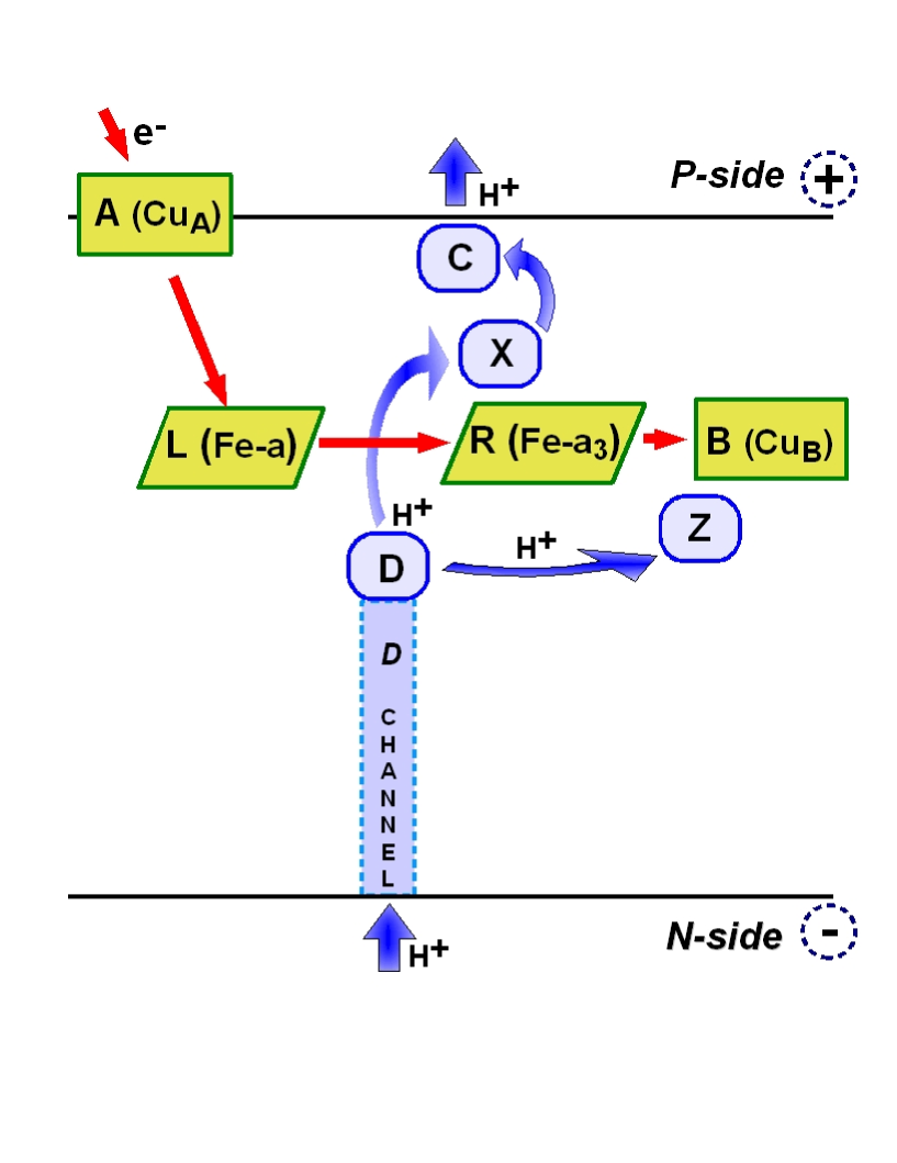
The last enzyme of the respiratory chain of animal cells and bacteria, cytochrome oxidase (CcO), operates as an efficient nanoscale machine converting electron energy into a transmembrane proton electrochemical gradient Alberts02 ; Nicholls92 ; Wik77 ; Wik04 ; Gennis04 ; Brez04 ; Branden06 . The ATP (adenosine triphosphate) synthase enzyme uses this energy to synthesize ATP molecules serving as the “energy currency” of the cell. The process of energy conversion starts when a molecular shuttle, cytochrome , delivers, one by one, high-energy electrons to a dinuclear copper center, CuA, located near a positive side (Pside) of the inner mitochondrial membrane (see Fig. 1). In recent time-resolved optical and electrometric studies BelPNAS07 of the CcO transition from the oxidized (O) state to the one-electron reduced form (E), a single electron is donated to the CuA redox center by a laser-activated molecule of ruthenium bispyridyl (RubiPy). Thereafter, in a few microseconds (10 s), a major part of an electron density (70%) is transferred from the CuA center to the low-spin heme (Fe-). Heme is located within the membrane domain at a distance about 2/3 of the membrane width, , counting from the N-side BelPNAS07 ; WV07 ; MedStuch05 . Within a time interval of approximately 150 s, about 60% of the electron population is transferred from heme to heme (Fe-). Heme , jointly with the next electron acceptor in line, a copper ion CuB, form a binuclear center (BNC, sites and in Fig. 1), serving as an active catalytic site for dioxygen reduction to water. The redox centers and CuB, are located approximately at the same distance from the N-side of the membrane as heme .
The next phase (with a time scale of the order of 800 s) is characterized by a complete electron transfer to the copper ion CuB. Time-resolved measurements BelPNAS07 show that the first “10 s” phase of the electron transfer process is not accompanied by a proton transfer, but the “slowness” of the second “150 s” and the third “800 s” phases hints to the proton participation during phases.
The proton path from the negative side of the membrane (N-side) toward the P-side (for pumped protons) and toward the binuclear center (for substrate or “chemical” protons) goes through the residue (for the enzyme BelPNAS07 ). These residues are located at the end of the so-called D-pathway (Fig. 1). A fraction of the substrate protons can also be delivered to the BNC via an additional K-pathway, which we will not consider here. The proton to be pumped is supposed to move from (schematically shown as the site “” in Fig 1) to an unknown protonable “pumping” site (likely a heme propionate), located above the BNC BelNat06 , and, thereafter, via an additional protonable site Siletsky04 ; Brez06 , to the P-side of the membrane. After a fast reprotonation from the D-channel, the residue can donate a substrate proton to the catalytic site near the BNC (probably, to an OH- ligand of CuB BelPNAS07 ; WV07 ). It is assumed BelPNAS07 ; WV07 that during the second “150 s” phase, the first (pre-pumped) proton moves from the residue (the site “D” in Fig. 1) to the pump site , whereas in the third “800 s” phase, the second (substrate or chemical) proton populates a catalytic site near the BNC. In the final phase, which occurs in 2.6 ms, the first proton (in ) is translocated (via ) to the P-side, which is characterized by a higher electrochemical potential than the N-side of the membrane.
As a result of all these processes, two protons are taken from the N-side of the membrane, and one electron is taken from the P-side, and eventually one proton is pumped to the P-side. Moreover, one proton and one electron are consumed at the catalytic site to finally produce a water molecule around the BNC. It should be noted that kinetic phases with similar time scales (sss) have been revealed in other CcO enzymes at various transition steps between the states of the enzyme Ruit02 ; Siletsky04 ; SalomBrez05 .
Kinetic data obtained in experiments BelPNAS07 ; Siletsky04 ; Ruit02 ; SalomBrez05 reflect important details of the still elusive proton pumping mechanism in cytochrome oxidase. To extract these details and gain a deeper insight into the operating principles of the CcO proton pump, it is necessary to compare results of experiments with theoretical predictions. In Ref. Olsson06 , a simplified empirical valence bond (EVB) effective potential was combined with a modified Marcus equation to model time-dependent electron and proton transfers in CcO in the range of milliseconds. However, this approach was applied to the single transfer event, not to the sequence of events, and the obtained time scale (one microsecond) differs by orders of magnitude from the experimental data (about 100 microseconds). A computational analysis of the CcO energetics was presented in Refs. Olsson07 ; Pisliakov08 ; SiegBlom07 ; SiegBlom08 ; Quenneville06 with molecular models reproducing energetic barriers for the proton transfer steps Olsson07 ; Pisliakov08 . The obtained energetic map of the proton and electron pathways in the CcO enzyme can be converted into a set of rate constants, which qualitatively explains the kinetics and unidirectionality of the pumping process. However, these studies do not result in a quantitative model of the efficient CcO proton pump. Moreover, the error range of these semi-microscopic calculations ( 2 kcal/mol) is sometimes higher than the difference between the energy barriers Pisliakov08 ; SiegBlom08 .
Kinetic models of the proton pumping process were also discussed in Ref. KimPNAS07 . Within the master equation approach, it was shown that the proton pumping effect can be achieved in a simplified system having one redox and two proton sites and, with a higher efficiency, 0.9, for the design with two redox and two protonable sites, which are electrostatically coupled to each other. However, this work does not contain any predictions for the kinetics of the pumping process in more realistic set-ups, with at least four redox sites (CuA, heme , heme , and CuB) and two protonable sites (a residue and a pump site ). To find proper parameters for the proton pump, the authors of Ref. KimPNAS07 resort to a Monte Carlo search in a multidimensional parameter space. It is hard to imagine, however, that a random search can provide a reasonable set of parameters which will comply with all physical restrictions of real pumps. In general, for comprehensive theoretical studies, it is preferable to determine the relevant parameters of the system using detailed microscopic calculations (see, e.g., Refs. Olsson06 ; Olsson07 ; Pisliakov08 ). However, the huge computational complexity of biological structures makes such an approach extremely difficult. In our paper, we include reasonable estimates for the system parameters into a model describing almost simultaneous electron and proton transfer processes and compare the obtained kinetics to experimentally observed time scales and site populations of cytochrome c oxidase BelPNAS07 .
The time evolution of the proton pumping process in CcO, related to the experimental data of Refs. BelPNAS07 ; Ruit02 ; Siletsky04 ; SalomBrez05 , was discussed in Refs. WV07 ; MedStuch05 ; SiegBlom07 ; SugStuch08 ; SiegBlom08 . In these works, the kinetics of the electron-proton system is broken down into a cascade of quasi-equilibrium states characterized by distributions of electrons and protons over the sites, as well as by a set of transition rates corresponding to specific kinetic phases. It should be emphasized, however, that many electron and proton transfers can be separated by only a nanosecond time scale, and, consequently, the experimentally observed kinetic rates comprise contributions of several almost-simultaneous individual electron and proton transfer events MedStuch05 ; SugStuch08 . Correspondingly, an approach taking into account the kinetic inseparability of electron and proton transitions can be useful for understanding recent experimental findings BelPNAS07 . We note that kinetic coefficients used in the theoretical analysis of Refs. MedStuch05 ; SiegBlom07 ; SugStuch08 ; SiegBlom08 were deduced from experiments without independent microscopic calculations of the heights of individual electron and proton barriers.
In the present paper, we analyze electron and proton kinetics in cytochrome oxidase within a simple physical model including four redox centers and four protonable sites electrostatically coupled to each other in the presence of a dissipative environment. Using the master equation approach, we reproduce all four kinetic phases observed in Ref. BelPNAS07 for a reasonable set of parameters. It should be emphasized that we have performed extensive numerical studies for a wide range of parameters and we found that our model of proton pumping is quite robust to significant variations of the parameters. The specific set of parameters presented below gives a very good agreement with the experimental data of Ref. BelPNAS07 . We consider a single cycle of events, which starts at with one electron transfer to the CuA center and finishes at the moment , when the redox site CuB is completely reduced. Notice that the injection of additional high-energy electrons is necessary to maintain this nonequilibrium state of the CcO enzyme. We also determine the efficiency of the proton pumping for our model and its dependencies on the temperature and transmembrane voltage.
The rest of paper is structured as follows. Our model and its parameters are presented in Section II. Results of numerical studies are shown in Section III and discussed in Section IV. Section V contains the conclusions of our work. The detailed derivation of the master equations and the measurable variables is presented in the Appendix. It should be noted that while the results of this paper are obtained in the classical regime, our approach (based on quantum transport theory) can be used to examine fine quantum effects and, consequently, the detailed derivation is worth presenting here.
II Model
As in the real CcO enzyme Iwata95 ; Tsukihara96 ; Yoshikawa98 ; Yoshikawa06 ; Ostermeier97 , the redox chain of the present model includes four centers: CuA (site ), heme (Fe-a, site ), heme (Fe-, site ), and CuB (site ), as schematically shown in Fig. 1. The transport chain for protons has four sites: (presumably related to the residue near the end of the D-pathway), (the pump site above the BNC), a protonable site placed on the way from the -site to the P-side of the membrane, and, finally, a protonable site located in the proximity of the BNC and related to the OH- ligand of CuB (see Fig. 1). The sites and serve as final destinations for the injected electron and for the substrate proton, respectively. We assume that the electron can be transferred between the pairs of redox states and , and , and ; and that protons can be translocated between the pairs of protonable sites and , and , as well as and .
To provide an “openness” of the CcO enzyme, which is inherent in the living systems KimPNAS07 , we allow proton transitions between the site and the negative side of the membrane as well as between the site and the positive side of the membrane. Protons are delivered to the catalytic site partially through the K-pathway Gennis04 ; WV07 . This channel can be incorporated into our model, but, for simplicity, it will be neglected. The N- and P- sides of the membrane play roles of proton reservoirs which work as a source (N-side) and a sink (P-side) of protons for the enzyme. The redox sites are disconnected from electron reservoirs, and only one electron is injected into the redox chain at the initial moment of time, .
With the condition of single-occupation of each individual site, the system can be populated with up to four protons. Following the setup of Ref. BelPNAS07 , we assume that CcO is populated with a single electron initially located on site . To quantitatively describe this system we introduce 64 basis states (see Appendix). The time evolution of the probability distribution over the basis states, , is governed by the system of master equations, Eq. (33), with the solution given by Eq. (35) in the Appendix. The time-dependent probability distribution allows us to determine the average populations of all electron and proton sites, and , as functions of time. We can also calculate the number of protons, , translocated to the positive side of the membrane [see Appendix, Eq. (37)]. The value of taken at the end of the pumping cycle () determines the pumping efficiency defined KimPNAS07 as the number of protons pumped across the membrane per electron consumed:
| (1) |
Note that the efficiency can take negative values in the case when protons move back from the positive side to the negative side of the membrane.
II.1 Electrostatic interaction
The electrostatic interaction between the redox () and protonable () sites plays a pivotal role in the electron-proton energy exchange. It should be noted that we consider here only direct Coulomb interactions between electron and proton subsystems and between protons themselves. This removes strict geometrical restrictions on the relative positions of electron and proton active sites imposed in our previous model PumpPRE08 based on the Förster-type energy exchange between electrons and protons. Microscopic calculations of the electrostatic parameters, and , involved in the Hamiltonian [see Appendix, Eq. (2)], require a detailed knowledge of the CcO structure complemented by the comprehensive dielectric map of the enzyme Olsson07 ; Warshel06 ; Schutz01 . Instead, we tune the Coulomb energies to get the best possible fitting of the time scales and site populations measured in the experiment BelPNAS07 . The obtained values of Coulomb parameters correlate well with information about the distances between the active sites Iwata95 ; Tsukihara96 ; Yoshikawa98 ; Yoshikawa06 ; Ostermeier97 for reasonable values of the effective dielectric constants.
To describe the experimentally observed kinetic phases of the pumping process, we assume that the coupling, meV, between the copper ion CuB and the catalytic site (likely an OH- ligand of CuB BelPNAS07 ; WV07 ) and the coupling, meV, between heme and the pump site are higher than the electrostatic energies meV and meV. Structural studies of the CcO enzyme Iwata95 ; Tsukihara96 ; Yoshikawa98 ; Yoshikawa06 ; Ostermeier97 performed at a resolution of about 2 Å show that the BNC redox sites (heme ), (CuB) and the protonable sites and are separated by a distance of the order of 6 Å. The value of the electrostatic coupling between these sites, meV, roughly corresponds to the effective dielectric constant, , which is of frequent use for a description of a dry protein interior Olsson07 ; SiegBlom08 ; Quenneville06 . It should be emphasized, however, that the concept of dielectric constant is not completely appropriate for a calculation of Coulomb potentials in the heterogeneous environment inside and near the BNC Warshel06 ; Schutz01 .
The distances, , between the residue (site D) and the sites and are almost the same: Å, Å Ostermeier97 ; Michel98 . We estimate the electrostatic coupling between these sites as meV, which corresponds to the higher dielectric constant We consider a smaller dielectric constant, , for the interaction, meV, between the sites and separated by the distance Å SiegBlom08 . Distant-dependent dielectric constants, , are common in protein electrostatics Olsson07 ; Warshel06 ; Schutz01 .
Note that here, as in the models of Refs. WV07 ; SiegBlom07 , the electrostatic coupling, between heme (site ) and the site is stronger than the interaction, between heme (site ) and the pump site . For the other parameters we choose the following values (in meV): The Coulomb energies and are assumed to be near 30 meV. Despite the fact that these energies are about or higher than the temperature energy scale, K meV, they have a minor influence on the performance of the model.
II.2 Energy levels of the sites
We assume that the difference (38) between the electrochemical potential of the P-side and the potential of the N-side of the membrane is about 210 meV at standard temperature, K, with meV and meV. This corresponds to voltage meV applied across the membrane. We include the electron charge in the parameter and measure voltage, along with other energies, in units of meV. According to Eqs. (39), the energy levels, and , of the electron and proton centers are shifted from their intrinsic values and depending on the voltage and on the positions of the active sites. To estimate the electron and proton energies, we take into account the facts Brez04 that cytochrome delivering electrons to the CcO enzyme has a redox potential of order of 250 meV, and that the total drop of electron energy between cytochrome and the dioxygen reduction site is about 550 meV. The equilibrium midpoint potentials BelPNAS07 ; WV07 of the CuA center ( meV) and heme ( meV) can also be used as a general guide for estimating energies Moser06 , although the real parameters can deviate from the estimated values.
We find that our model performs with the high efficiency, , and reproduces all experimentally observed kinetic phases BelPNAS07 for the following set of electron intrinsic energies (in meV): and for the following energies of protonable sites (in meV): and It should be noted that in the presence of the transmembrane voltage, meV, the electron energy levels of and sites, are close to the values extracted from equilibrium redox titrations (see also Ref. Farver06 , where an estimation, meV, has been obtained). For energies of other redox sites we use the values: The energies of the protonable sites are also shifted with voltage, meV, present: and . It should be stressed that the energy, , of the pump site is set to be higher than the potentials of the proton reservoirs on both sides of the membrane: However, the presence of an electron on the site decreases the proton energy to the level, meV, which is below the energy of the -site and below the electrochemical potential, meV, of the N-side of the membrane. As a result, the pump site is populated with a pre-pumped proton. When the chemical proton moves to the site Z and the electron is transferred to the -site, the energy level of the -site returns to the initial position, meV, since the electron and proton charges of the catalytic site compensate each other, . The high-energy pre-pumped proton can now move to the site and, after that, to the P-side of the membrane characterized by the potential meV. A large energy gap, meV, significantly suppresses the return of the -proton to the site and to the N-side of the membrane.
II.3 Reorganization energies and transition rates
Part of the energy delivered to the redox center CuA at the initial time, , is dissipated to an environment characterized by sets of electron () and proton () reorganization energies. To be efficient, the proton pumping process should occur with minimal energy dissipation. It is shown in Ref. Jas05 that the reorganization energy for the to electron transfer in the CcO enzyme can be as low as 100 meV. Similar estimates apply for the proton reorganization energies Silverman00 ; Wraight05 . Here, we use the higher energy parameter, meV, for the A-to-L transfer and accept the lower value, meV, for other electron and proton transitions. It is argued in Refs. Farver06 ; Larsson95 ; Ramirez95 , that for the Cu heme electron transition the reorganization energy must be in the range from 150 meV to 500 meV, which is much lower than the typical values of the reorganization energy for electron transfers in protein. The low values of electron reorganization energies ( – 4 kcal/mol) have also been calculated for electron transfer reactions in Rhodobacter sphaeroides Warshel06 .
To reproduce the initial kinetic phases, we use the following tunneling energies: eV, and eV. The parameters and describe the electron transfers, which are coupled to the slower proton transitions characterized by the energy scales: eV, and eV. It should be noted that the electron transfer between heme and heme can occur in a nanosecond time scale Pilet04 . The hydrogen-bonded chains in proteins are also able to conduct protons in nanoseconds or faster Nagle78 ; Zundel95 .
We also select the values ms-1 for the parameters and , which determine the flow of protons through the enzyme. These parameters and are of the same order as some of the transition rates used in Ref. KimPNAS07 .
III Results
III.1 Four kinetic phases
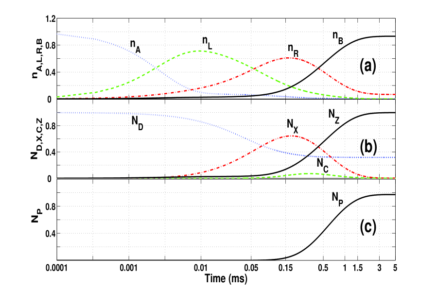
In Fig. 2, starting at , we show a process of population and depopulation of the electron, , and proton, , sites as well as the time dependence of the average number of protons pumped to the positive side of the membrane, . From here on we drop the brackets denoting the averaging over the environmental fluctuations and over the states of the proton reservoirs. The calculations are performed for the standard conditions ( meV, meV, , ) and for the transmembrane voltage meV. We assume that initially a single electron is located at the site (CuA), and a proton occupies the site . This means that at only one element of the density matrix is not equal to zero:
During the first phase of the process the electron moves from the site to the site (heme ). In 10 s near 70% of the electron density is transferred to the heme (site ) with the remaining 30 percent distributed almost equally between the site (CuA) and the site (heme ). This corresponds roughly to the 70 percent electron population of heme after the first s phase observed experimentally in Ref. BelPNAS07 . No pronounced changes in populations of the protonable sites accompany this stage [see Fig. 2 (b)].
The second phase of the electron transfer is postponed by the time 150 s, despite the fast intrinsic transition rate between the and redox sites. Besides the 55 meV potential difference between the sites and , the electron transfer in this phase is hampered by the involvement of protons. It is evident from Figs. 2a and 2b that, with a microsecond delay, the slightly uphill electron transfer from the site to the site is followed by the proton translocation from the site ( meV) to the pump site having much higher initial energy, meV. This transition has been made possible by the strong - Coulomb attraction ( = 555 meV) lowering the effective energies of both electron and proton sites. In line with the experimental data BelPNAS07 at s, the electron density is located mainly on the site (60%) and partially on the sites (20%), and on the site (15%). The site is practically empty at this stage. It is important that at almost the same moment of time (s) the population of the protonable pump site also reaches its maximum (65%).
It is evident from Fig. 2b that the occupation of the pump site is accompanied by the monotonic population of the the protonable catalytic site , thus lowering the energy of the redox site from its initial level, meV, to the final value of the order of meV (see also Fig. 3). The population of the -site, , closely follows (with a small delay) the population of the proton catalytic site (see Figs. 2a and 2b). It can be seen from Fig. 2b that in 300 microseconds the pumped proton moves from the site to the transient site , placed between and the P-side of the membrane, and after that to the positive side of the membrane.
In the third phase ( ms), the substrate (chemical) proton (Fig. 2b) occupies the catalytic site , . Then, with a microsecond delay, the electron (Fig. 2a) is transferred, , to the -center (CuB), so that the heme is practically re-oxidized, . This stage is correlated with the s phase mentioned in Ref. BelPNAS07 .
In the fourth phase ( ms), the pumped proton (Fig. 2c) moves to the positive site of the membrane, , the substrate proton populates the site , , and the electron is almost completely transferred to the site , . On average, about 1.3 protons are taken from the N-side of the membrane during the whole process.
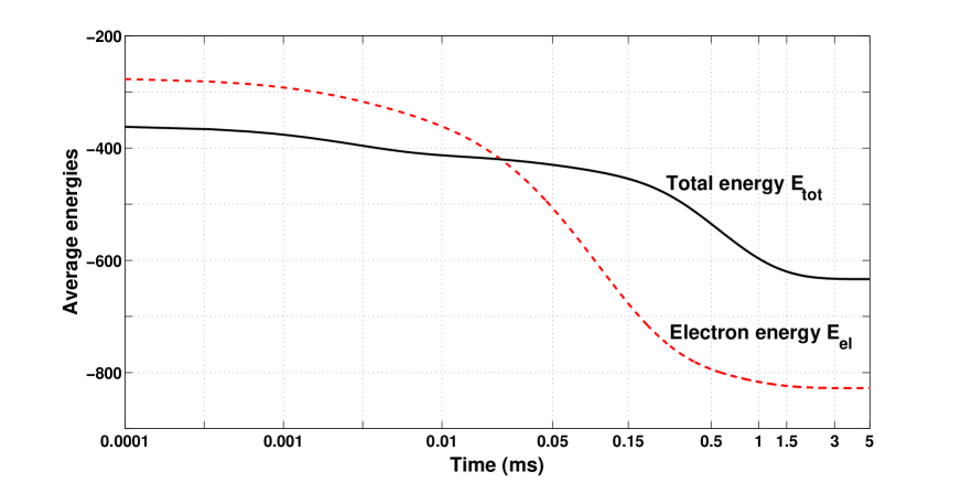
The variations of the average electron energy, and the total energy of the system,
with time are shown in Fig. 3. Here is the basic Hamiltonian of the system (2), is the Hamiltonian of the electron component (3), and are the average numbers of protons (37) translocated to the P- or N-side of the membrane, respectively. At the beginning, the electron has energy
and at the end of the process its energy sinks to the level
with the total drop meV, corresponding to the experimental value Brez04 . The total energy of the system, , shows a decrease of the order of meV, which is less than the drop of electron energy since one proton gains the energy during its pumping to the positive side of the membrane.
III.2 Pumping efficiency
It follows from Fig. 2(c), that at ms, the average number of pumped protons, , reaches its peak value, which can be used as a definition KimPNAS07 of the pumping efficiency : . According to this definition, the present model demonstrates an almost-perfect performance with an efficiency at K, meV, meV. This is comparable to the efficiency of cytochrome c oxidase Wik77 ; Brez04 pumping one proton across the membrane per one electron consumed at the oxygen reduction site. We find that the definition of the efficiency introduced above is not sensitive to the choice of the specific moment ms, since the number of pumped protons, , does not decrease noticeably with time during the interval from 5 ms to more than 100 ms at the standard conditions.
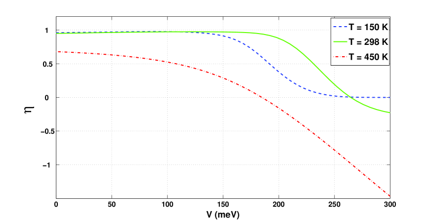
In Fig. 4 we plot the pumping efficiency versus the transmembrane voltage at three different temperatures: K (blue dashed line), K (green continuous curve), and K (red dash-dotted line). We assume that the electrochemical gradient varies in accordance to Eq. (38) where At K the pumping efficiency is almost constant at low voltages, meV, with a subsequent drop at high voltages. The pump works better at room temperatures, K, and keeps the efficiency steady up to voltages meV. Notice that in this case the efficiency , which is proportional to the average number of pumped protons, becomes negative at meV. The performance of the model is significantly deteriorated at high temperatures, K, when the proton flow is reversed starting with the relatively low voltage gradient, meV.
IV Discussion
The obtained time evolution of the electron and proton populations (see Fig. 2) features four experimentally observed phases of the proton pumping process: the first “s” phase, when the electron is transferred from CuA (site ) to heme a (site ); the second “s” phase when the electron moves from heme a to heme (site ), and, with a microsecond delay, a proton partially occupies the pump site ; the third “s” phase when the “chemical” proton is transferred to the catalytic sites and, a slightly later, the electron is transferred to the ultimate electron acceptor CuB. In the fourth phase, at ms, the pre-pumped proton is released to the P-side of the membrane.
It should be emphasized that, contrary to the models proposed in Refs.BelPNAS07 ; WV07 ; SugStuch08 , this process cannot be described as a sequence of transitions between clearly defined quasi-equilibrium states since many electron and proton transfers occur in a very short time one after the other. The present theoretical model, which includes four redox sites (two copper centers and two hemes) and four protonable sites, is able to explain the efficient performance () of the real cytochrome c oxidase Wik77 pumping almost one proton per one electron consumed against the electric potential difference, meV, and against the transmembrane electrochemical gradient, meV. We stress that all four kinetic phases appear naturally in our model for a reasonable set of the system parameters without artificial inclusions of consequent transfer processes.
The mechanism of the proton pumping analyzed above is based on the direct electrostatic interaction between the redox and protonable sites, especially between the electron located on the site (heme ) and the proton located on the pump site . The Coulomb coupling between the redox site CuB and the protonable catalytic site plays a very important role as well. The proton to be pumped is sequentially translocated to the P-side of the membrane from the sites and . At the beginning of the process these sites are empty since their energy levels are assumed to be higher than the energy levels of the proton source ( and ) and the proton drain (). After the first “s” phase the energy level of the -site is slightly ( meV) lower than the energy level of the -site. However, an interaction with the environment facilitates the slow electron transfer to the site . The population of the site with the electron is accompanied by the lowering of the -site energy level followed by the proton translocation from the site to the pump site . Because of the strong - electrostatic attraction, the effective energy of the -electron drops below the energy of the -site, which results in the second “s” phase where the major part (%) of the electron density is concentrated on the site , and the pump site is partially (%) populated with a proton. The electron transfer to the site also leads to lowering the energy of -site, thus inducing a monotonous population of the catalytic protonable site . No switch redirecting protons to the site or to the site (as proposed in Ref. WVH03 ) is needed here because both of these sites can be populated from the site .
It should also be emphasized that these three processes: the electron transfer to the -site, the occupation of the pump site , and the translocation of a proton to the -site, are strongly correlated in time. The proton transfer to the -site digs a deep potential well for the electron at the site , and in the third ( ms) phase the electron falls into this well. Afterwards, the Coulomb attraction between the pre-pumped -proton and the electron is almost compensated by the electrostatic repulsion between and protons, and the energy level of the -proton returns to its original high value. The reverse translocation of the -proton to the site is strictly suppressed since now the energy difference between the sites and ( meV) significantly exceeds the reorganization energy as well as the temperature broadening, , of the transition rates in Eq. (28). However, the pre-pumped proton can easily move to the slightly ( meV) lower energy level , and, after this, to the positive side of the membrane characterized by the even lower electrochemical potential meV. Our model does not require any nonlinear gates WVH03 to prevent a proton leakage from the positive to the negative side of the membrane.
V Conclusion
We have analyzed a simple model describing the kinetics of the proton pumping process in cytochrome oxidase initiated by a single-electron injection. Within our model, this electron is subsequently transferred along four sites electrostatically coupled to four protonable sites. We have shown that the energy loss by this electron facilitates the proton transfer against the transmembrane voltage from the negative to the positive sides of the membrane with the efficiency In contrast to previous studies, we have not broken the electron and proton transfers into a series of transitions between the independent quasi-equilibrium states but examined inseparable dynamics of the pumping process. We have derived the master equations of motion and solved them numerically for a reasonable set of the system parameters. The obtained time evolution naturally encompasses all four experimentally observed kinetic phases.
Appendix A Master equations
The kinetics of charge transfer in the CcO enzyme can be described by a set of master equations KimPNAS07 ; Haken04 ; Ferreira06 . For completeness we present here a derivation of these equations. We start from the formalism of second quantization PumpPRE08 ; Wingr93 ; FlagPRE08 , even though in this paper we only discuss the classical results, with an examination of quantum coherent effects to be performed in the future. Electrons, located on the redox sites , are described by the creation and annihilation Fermi operators , and protons located on the protonable sites () are described by the creation and annihilation Fermi operators . The spin degrees of freedom are neglected; thus, each site can only be occupied by a single particle. The electron population of the -site, , is expressed as , and for a proton population on site , we have the relation: . Protons on the negative (N) and on the positive (P) side of the membrane ( = N,P) are continuously distributed over the space of an additional “quasi-wavenumber” parameter and characterized by the creation and annihilation Fermi operators with the density operator .
A.1 Hamiltonian of the system
The total Hamiltonian of the electron-proton system incorporates a basic term,
| (2) |
where the first and second terms describe the electron () and proton () sites with energies and , respectively, and the third and fourth terms are responsible for the Coulomb interaction of protons with each other and the electron, respectively. It should be noted that in our single-electron model there is no inter-electron Coulomb interaction. We will also calculate the energy of the electron component, which is determined by the Hamiltonian
| (3) |
For protons in the N-side and P-side reservoirs we introduce the Hamiltonian
| (4) |
with the energy spectrum , whereas proton transitions between site and the N-side of the membrane, and site and the P-side are given by the transfer Hamiltonian
| (5) |
characterized by the coefficients and . The component
| (6) |
is responsible for electron tunneling between the pairs () of sites -, -, -, and for proton transitions between the pairs () of sites -, -, and -, with the corresponding amplitudes (for electrons) and (for protons), where and .
Protons are delivered from a solution to the active site by the water-filled D-channel Gennis04 ; Branden06 . It was argued Brez06 ; Nagle78 ; Wright06 that the D-channel contains hydrogen-bonded chains of water molecules, which can convey protons via the Grotthuss mechanism. In this case, the proton transfer is considered as a collective motion of a positive charge through the chain, but not as a motion of an individual proton. According to another point of view (see Refs. Olsson07 ; Olsson05 ; Kato06 ; BraunSand04 ), the proper orientation of water molecules required for the Grotthuss mechanism is characterized by a much smaller energetic penalty than the electrostatic barriers associated with a proton transfer through the channel. Thus, the dominant contribution to the kinetic rate of the proton transport in proteins is provided by the electrostatic energy. In the present work we model proton transitions (between the site and the N-side as well as between the site and the P-side of the membrane) by the Hamiltonian (5) with matrix elements that do not specify the transfer origin.
The transport of protons between the active sites -, -, and - are described by phenomenological coefficients in the Hamiltonian (6). To obtain kinetic rates for proton transitions between active sites in the presence of an environment, we resort to the Marcus formulation of the problem. The relevant approach based on the empirical valence bond method Warshel80 has been developed in Ref. BraunSand04 . As shown in Refs. Olsson06 ; Olsson07 ; Olsson05 , the modified Marcus relations can be successfully applied for modelling the proton transfer steps in cytochrome oxidase.
A.2 Environment
To take into account the interaction of the electron-proton system with its environment, we introduce a term :
| (7) |
where is the total number of protons in the -reservoir ( = N, P). The environment is represented as a set of harmonic oscillators Garg85 ; Krish01 with coordinates , momenta , masses , and frequencies . The shifts , , and define coupling strengths of electrons and protons to the environment. The total Hamiltonian is the sum of all above-mentioned components:
| (8) |
With the unitary transformation,
| (9) |
the total Hamiltonian, can be transformed to the form
| (10) | |||||
where the operators,
| (11) |
describe the effect of the environment on the electron and proton transitions. The protonable site is located near the P-side of the membrane, and the site is tightly coupled to the N-side by the D-channel. It is reasonable to assume, therefore, that -to-P and N-to- proton transitions have a negligible effect on the equilibrium position of the -oscillator of the environment: so that the corresponding phase factors in Eq. (11) related to the Hamiltonian and to the total Hamiltonian (10) can be omitted.
A.3 Basis states and eigenenergies
To quantitatively analyze the system with a single electron and with up to four protons we introduce a basis of 64 eigenstates of the Hamiltonian : Here is the vacuum state of the system with no electrons and no protons, is the state with an electron on site , is the state with an electron on site and a proton on site , has one electron on site and a proton on site , describes the state with an electron on site and a proton on site , and so on. Finally, is the state with a single electron on site and with one proton on each site and (i.e., a total of four protons). The state has the eigenenergy , the state has the energy and the last state , fully loaded with four protons, has the energy
The Hamiltonian (2) is diagonal in the new basis:
| (12) |
Other operators may have a non-diagonal form in the new basis, for example,
| (13) |
where
| (14) |
Here indices and sweep all integers from 1 to 64.
A.4 Electron and proton transitions
In addition to the diagonal parts and , the total Hamiltonian of the system contains the term responsible for the proton transitions between the N-side of the membrane and the site , and between the P-side and the site :
| (15) |
as well as the off-diagonal term describing the tunneling of electrons and the transfer of protons between the active sites,
| (16) |
Here the operator is represented by a linear combination of the bath operators [see Eqs. (11)], multiplied by the non-diagonal () transition matrix elements :
| (17) | |||||
It should also be noted that operators of the N and P proton reservoirs, and cannot be completely expressed in terms of the basis operators .
A.5 Derivation of the master equations
A probability to find the electron-proton system in the state is determined by the diagonal operator averaged over the states of the environment and over the distributions of protons on both, N and P, sides of the membrane. The time evolution of the operator is governed by the Heisenberg equation
| (18) |
To derive a master equation for the probabilities , we have to average Eq. (18) and calculate the correlation functions of the environment operators (17) and the operators of the system . The transition coefficients, and are supposed to be much smaller than the energy scales given by the basis spectrum This means that the effective interactions with the N and P proton reservoirs [see Eq. (15)] and with the bath of oscillators (see Eqs. (16),(17)) can be treated as a perturbation. In the framework of the theory of open quantum systems proposed in Ref. ES81 the correlation function (with , no summation over and ) can be written in the form
| (19) | |||||
Here is a variable of the free environment (with no coupling to the electron-proton system), and is the Heaviside unit step function. We introduce the following notations for a cumulant function of two operators and :
and for a commutator:
In Eq. (19) we take into account the backaction of the bath in a contrast to the approach of Ref. PumpPRE08 where this backaction is not included into consideration. Due to significant decoherence effects, off-diagonal elements of the density matrix, , disappear very fast. Because of this, the first term in the r.h.s. of Eq. (19) can be neglected despite the non-zero value of the average unperturbed operator . The times and involved in the integrands of Eq. (19) are separated by the correlation time of the correlators, which are similar to the function . The timescale is determined by the reorganization energy and temperature : (see Refs. Marcus56 ; Krish01 and Eq. (24) below). We assume that transitions between the active sites have a negligible effect on the time evolution of the operator between the times and , which are separated by the correlation time . Thus, the correlation functions and commutators of the operators and can be calculated using free-evolving functions:
where For the correlator (19) we obtain the formula
| (20) |
With Eq. (17), we can express the cumulant in terms of cumulant functions of the unperturbed bath operators :
| (21) |
The correlation function has a similar form, with cumulants being replaced by . Using the definitions (11) of the bath operators we can calculate their correlation functions. In particular,
| (22) |
where
| (23) |
and is the temperature of the environment (). These expressions can be simplified in the high-temperature limit when the thermal fluctuations are much faster () than the environment modes coupled to the charge transfer Krish01 : , and, correspondingly,
| (24) |
We introduce here the reorganization energy,
| (25) |
corresponding to the electron transition from the site to the site . Similar parameters can also be introduced for other electron transitions: from to , from to , as well as for proton transitions between sites and , and , and between and the catalytic site .
After a sequential substitution of Eqs. (24), (21), (20) into the averaged equation (18), we obtain the contribution of the inter-site transfers into the master equation
| (26) |
where the combined rate contains contributions of all possible electron and proton transitions,
| (27) |
The rates corresponding to the specific electron transfers, and the rates related to the proton transfers, are all determined by the Marcus equations Marcus56 ; Krish01 with coefficients given by the appropriate transition matrices. In particular,
| (28) |
| (29) |
It should be noted that the ratio between the transposed rate coefficients is equal to the Boltzmann factor, as
which results in the Boltzmann distribution for the equilibrium density matrix of the system.
The contribution, , of proton transitions between the site and the N-side of the membrane and between the exit site and the P-side of the membrane to the master equation (26) can be calculated with the methods of quantum transport theory Wingr93 ; PumpPRE08 ; FlagPRE08 . The coupling to the proton reservoirs is described by the relaxation matrix,
| (30) | |||||
where the energy-independent coefficient,
| (31) |
determines the rate of a proton delivery to the -site ( = N) or the rate of a proton removal from the -site ( = P). We assume here that protons on the -side of the membrane are described by the Fermi distribution,
| (32) |
characterized by a chemical potential .
A.6 Algebraic solution of the master equations
Determination of the time-dependent solution of the master equations (33) can be reduced to a purely algebraic problem. To accomplish this, we rewrite the equations (33) in the form
| (34) |
with a total relaxation matrix , where at , and The vector with the elements can be represented as a sum of the steady-state part, , and the time-dependent deviation , as Both the total probability vector and its steady-state value satisfy the normalization condition: The steady-state distribution can be found from the matrix equation , and for a time-dependent part we have a rate equation in the form Using the unitary operator, , the matrix can be transformed to the diagonal form with as the diagonal elements. This transformation should be accompanied by the transformation of the vector as Then, the vector obeys the diagonal equation with a simple solution for its -component: Correspondingly, the time evolution of the probability vector from its initial value is described by the formula
| (35) |
where , and is the diagonal matrix with the elements It should be noted that and where is the 6464 unit matrix.
A.7 Proton current
The time-dependent populations, and , of all redox and protonable sites in the model are expressed in terms of the evolving probability distribution . We recall that the index labels the redox sites = (CuA), (heme ), (heme ), and (CuB). The index labels the protonable sites and . Finally, the index labels the two sides of the membrane = N, P. With the density matrix probability distributions, , over the states, , of the system we can also find the proton flows from the N-side and P-side of the membrane into the system, where is the total number of protons on the -side of the membrane: . Using techniques developed in quantum transport theory Wingr93 ; PumpPRE08 , we obtain the formulas for the proton currents and :
| (36) |
Note that these currents depend on the time-dependent probability distribution and, accordingly, they also vary with time. The total number of protons, , transferred to the -side of the membrane ( = P,N) is calculated as the integral of the corresponding current:
| (37) |
A.8 Proton-motive force
The proton-motive force across the membrane can be defined as a difference of electrochemical potentials and involved in the Fermi distributions (32) of the proton reservoirs: . This gradient includes the transmembrane concentration difference () and the transmembrane voltage :
| (38) |
Here and are the gas and Faraday constant, respectively, and is the temperature (in degrees Kelvin, ) Alberts02 ; Nicholls92 . Both energy parameters, and , are measured in meV. At the standard conditions (), the concentration gradient contributes about 60 meV per -unit. This results in the transmembrane voltage meV, provided that the total proton-motive force, , is about 210 meV, and Alberts02 .
The transmembrane voltage, elevates the energies of protonable sites adjacent to the P-side and lowers the energies of the proton sites located near the N-side KimPNAS07 . The electron sites are simultaneously experiencing the opposite effect, for the same . As a result the electron energy levels, , and the proton energies, , involved in the Hamiltonian (2) are shifted from their initial values, and :
| (39) |
where is the membrane width. The positions of the redox and protonable sites, and , are counted here from the middle of the membrane with the x-axis directed toward the P-side: BelPNAS07 ; MedStuch05 .
Acknowledgements.
This work was supported in part by the National Security Agency (NSA), Laboratory of Physical Science (LPS), Army Research Office (ARO), National Science Foundation (NSF) grant No. 0726909, and JSPS-RFBR 06-02-91200. L.M. is partially supported by the NSF NIRT, grant ECS-0609146.
References
- (1) B. Alberts, A. Johnson, J. Lewis, M. Raff, K. Roberts, and P. Walter, Molecular Biology of the Cell (Garland Science, New York, 2002), Ch. 14.
- (2) D.G. Nicholls and S.J. Ferguson, Bioenergetics 2 (Academic Press, London, 1992).
- (3) M. Wikström, Nature (London) 266, 271 (1977).
- (4) M. Wikström, Biochim. Biophys. Acta 1655, 241 (2004).
- (5) R.B. Gennis, Frontiers in Bioscience 9, 581 (2004).
- (6) P. Brzezinski, Trends Biochem. Sci. 29, 380 (2004).
- (7) G. Bränden, R.B. Gennis, and P. Brzezinski, Biochim. Biophys. Acta 1757, 1052 (2006).
- (8) I. Belevich, D. A. Bloch, N. Belevich, M. Wikström, and M.I. Verkhovsky, Proc. Natl. Acad. Sci. U.S.A. 104, 2685 (2007).
- (9) M. Wikström and M.I. Verkhovsky, Biochim. Biophys. Acta 1767, 1200 (2007).
- (10) D.M. Medvedev, E.S. Medvedev, A.I. Kotelnikov, and A.A. Stuchebrukhov, Biochim. Biophys. Acta 1710, 47 (2005).
- (11) I. Belevich, M.I. Verkhovsky, and M. Wikström, Nature (London) 440, 829 (2006).
- (12) S.A. Siletsky, A.S. Pawate, K. Weiss, R.G. Gennis, and A.A. Konstantinov, J. Biol. Chem. 279, 52558 (2004).
- (13) P. Brzezinski and P. Ädelroth, Curr. Opin. Struct. Biol. 16, 465 (2006).
- (14) M. Ruitenberg, A. Kannt, E. Bamberg, K. Fendler, and H. Michel, Nature (London) 417, 99 (2002).
- (15) L. Salomonsson, K. Faxen, P. Ädelroth, and P. Brzezinski, Proc. Natl. Acad. Sci. U.S.A. 102, 17624 (2005).
- (16) M.H.M. Olsson and A. Warshel, Proc. Natl. Acad. Sci. U.S.A. 103, 6500 (2006).
- (17) M.H.M. Olsson, P.E.M. Siegbahn, M.R.A. Blomberg, and A. Warshel, Biochim. Biophys. Acta 1767, 244 (2007).
- (18) A.V. Pisliakov, P.K. Sharma, Z.T. Chu, M. Haranczuk, and A. Warshel, Proc. Natl. Acad. Sci. U.S.A. 105, 7726 (2008).
- (19) P.E.M. Siegbahn and M.R.A. Blomberg, Biochim. Biophys. Acta 1767, 1143 (2007).
- (20) P.E.M. Siegbahn and M.R.A. Blomberg, J. Phys. Chem. A 112, 12772 (2008).
- (21) J. Quenneville, D.M. Popovic, and A.A. Stuchebrukhov, Biochim. Biophys. Acta 1757, 1035 (2006).
- (22) Y.C. Kim, M. Wikström, and G. Hummer, Proc. Natl. Acad. Sci. U.S.A. 104, 2169 (2007).
- (23) R. Sugitani, E.S. Medvedev, and A.A. Stuchebrukhov, Biochim. Biophys. Acta 1777, 1129 (2008).
- (24) S. Iwata, C. Ostermeier, B. Ludwig, and H. Michel, Nature (London) 376, 660 (1995).
- (25) T. Tsukihara, H. Aoyama, E. Yamashita, T. Tomizaki, H. Yamaguchi, K. Shinzawa-Itoh, R. Nakashima, R. Yaono, and S. Yoshikawa, Science 272, 1136 (1996).
- (26) S. Yoshikawa, K. Shinzawa-Itoh, R. Nakashima, R. Yaono, E. Yamashita, N. Inoue, M. Yao, M.J. Fei, C.P. Libeu, T. Mizushima, H. Yamaguchi, T. Tomizaki, and T. Tsukihara, Science 280, 1723 (1998).
- (27) S. Yoshikawa, K. Muramoto, K. Shinzawa-Itoh, H. Aoyama, T. Tsukihara, K. Shimokata, Y. Katayama, and H. Shimada, Biochim. Biophys. Acta 1757, 1110 (2006).
- (28) C. Ostermeier, A. Harrenga, U. Ermler, and H. Michel, Proc. Natl. Acad. Sci. U.S.A. 94, 10547 (1998).
- (29) A.Yu. Smirnov, L.G. Mourokh, and F. Nori, Phys. Rev. E 77, 011919 (2008).
- (30) A. Warshel, P.K. Sharma, M. Kato, and W.W. Parson, Biochim. Biophys. Acta 1764, 1647 (2006).
- (31) C.N. Schutz and A. Warshel, Proteins 44, 400 (2001).
- (32) H. Michel, Proc. Natl. Acad. Sci. U.S.A. 95, 12819 (1998).
- (33) C.C. Moser, T.A. Farid, S.E. Chobot, and P.L. Dutton, Biochim. Biophys. Acta 1757, 1096 (2006).
- (34) O. Farver, E. Grell, B. Ludwig, H. Michel, and I. Pecht, Biophys. J. 90, 2131 (2006).
- (35) A. Jasaitis, F. Rapaport, E. Pilet, U. Liebl, and M.H. Vos, Proc. Natl. Acad. Sci. U.S.A. 102, 10882 (2005).
- (36) D.N. Silverman, Biochim. Biophys. Acta 1458, 88 (2000).
- (37) C.A. Wraight, in Biophysical and Structural Aspects of Bioenergetics, edited by M. Wikström (RSC Publishing, Cambridge, 2005).
- (38) S. Larsson, B. Källebring, P. Wittung, and B.G. Malmström, Proc. Natl. Acad. Sci. U.S.A. 92, 7167 (1995).
- (39) B.E. Ramirez, B.G. Malmström, J.R. Winkler, and H.B. Gray, Proc. Natl. Acad. Sci. U.S.A. 92, 11949 (1995).
- (40) E. Pilet, A. Jasaitis, U. Liebl, and M.H. Vos, Proc. Natl. Acad. Sci. U.S.A. 101, 16198 (2004).
- (41) J.F. Nagle and H.J. Morowitz, Proc. Natl. Acad. Sci. U.S.A. 75, 298 (1978).
- (42) F. Bartl, G. Deckers-Hebestreit, K. Altendorf, and G. Zundel, Biophys. J. 68, 104 (1995).
- (43) M. Wikström, M.I. Verkhovsky, and G. Hummer, Biochim. Biophys. Acta 1604, 61 (2003).
- (44) H. Haken Synergetics (Springer-Verlag, Berlin, 2004).
- (45) A.M. Ferreira and D. Bashford, J. Am. Chem. Soc. 128, 16778 (2006).
- (46) N.S. Wingreen, A.-P. Jauho, and Y. Meir, Phys. Rev. B 48, 8487 (1993).
- (47) A.Yu. Smirnov, S. Savel’ev, L.G. Mourokh, and F. Nori, Phys. Rev. E 78, 031921 (2008).
- (48) C.A. Wraight, Biochim. Biophys. Acta 1757, 886 (2006).
- (49) M.H.M. Olsson, P.K. Sharma, and A. Warshel, FEBS Letters 579, 2026 (2005).
- (50) M. Kato, A.V. Pisliakov, and A. Warshel, Proteins 64, 829 (2006).
- (51) S. Braun-Sand, M. Strajbl, and A. Warshel, Biophys. J. 87, 2221 (2004).
- (52) A. Warshel and R.M. Weiss, J. Am. Chem. Soc. 102, 6218 (1980).
- (53) A. Garg, J. N. Onuchic, and V. Ambegaokar, J. Chem. Phys. 83, 4491 (1985).
- (54) D. A. Cherepanov, L.I. Krishtalik, and A. Y. Mulkidjanian, Biophys. J. 80, 1033 (2001).
- (55) G.F. Efremov and A.Yu. Smirnov, Sov. Phys. JETP 53, 547 (1981).
- (56) R. Marcus, J. Chem. Phys. 24, 966 (1956).