Interferometry with independent Bose-Einstein condensates: parity as an EPR/Bell quantum variable

Abstract

When independent Bose-Einstein condensates (BEC), described quantum mechanically by Fock (number) states, are sent into interferometers, the measurement of the output port at which the particles are detected provides a binary measurement, with two possible results $\pm 1$. With two interferometers and two BEC’s, the parity (product of all results obtained at each interferometer) has all the features of an Einstein-Podolsky-Rosen quantity, with perfect correlations predicted by quantum mechanics when the settings (phase shifts of the interferometers) are the same. When they are different, significant violations of Bell inequalities are obtained. These violations do not tend to zero when the number $N$ of particles increases, and can therefore be obtained with arbitrarily large systems, but a condition is that all particles should be detected. We discuss the general experimental requirements for observing such effects, the necessary detection of all particles in correlation, the role of the pixels of the CCD detectors, and that of the alignments of the interferometers in terms of matching of the wave fronts of the sources in the detection regions.

Another scheme involving three interferometers and three BEC’s is discussed; it leads to Greenberger-Horne-Zeilinger (GHZ) sign contradictions, as in the usual GHZ case with three particles, but for an arbitrarily large number of them. Finally, generalizations of the Hardy impossibilities to an arbitrarily large number of particles are introduced. BEC’s provide a large versality for observing violations of local realism in a variety of experimental arrangements.

PACS numbers: 03.65.Ud, 03.75.Gg, 42.50.Xa

The original Einstein-Podolsky-Rosen (EPR) argument [1] considers a system of two microscopic particles that are correlated; assuming that various types of measurements are performed on this system in remote locations, and using local realism, it shows that the system contains more “elements of reality” than those contained in quantum mechanics. Bohr gave a refutation of the argument [2] by pointing out that intrinsic physical properties should not be attributed to microscopic systems, independently of their measurement apparatuses; in his view of quantum mechanics (often called “orthodox”), the notion of reality introduced by EPR is inappropriate. Later, Bell extended the EPR argument and used inequalities to show that local realism and quantum mechanics may sometimes lead to contradictory predictions [3]. Using pairs of correlated photons emitted in a cascade, Clauser et al. [5] checked that, even in this case, the results of quantum mechanics are correct; other experiments leading to the same conclusion were performed by Fry et al. [6], Aspect et al. [7], and many others. The body of all results is now such that it is generally agreed that violations of the Bell inequalities do occur in Nature, even if experiments are never perfect and if “loopholes” (such as sample bias [8, 9, 10]) can still be invoked in principle. All these experiments were made with a small number of particles, generally a pair of photons, so that Bohr’s point of view directly applies to them.

In this article, as in [11] we consider systems made of an arbitrarily large number of particles, and study some of their variables that can lead to an EPR argument and Bell inequalities. Mermin [12] has also considered a physical system made of many particles with spins, assuming that the initial state is a so called GHZ state [13, 14]; another many-particle quantum state has been studied by Drummond [15]. Nevertheless, it turns out that considering a double Fock state (DFS) with spins, instead of these states, sheds interesting new light on the Einstein-Bohr debate. The reason is that, in this case, the EPR elements of reality can be macroscopic, for instance the total angular momentum (or magnetization) contained in a large region of space; even if not measured, such macroscopic quantities presumably possess physical reality, which gives even more strength to the EPR argument. Moreover, one can no longer invoke the huge difference of scales between the measured properties and the measurement apparatuses, and Bohr’s refutation becomes less plausible.

Double Fock states with spins also lead to violations of the Bell inequalities [16, 17], so that they are appropriate for experimental tests of quantum violations of local realism. A difficulty, nevertheless, is that the violations require that all $N$ spins be measured in $N$ different regions of space, which may be very difficult experimentally if $N$ exceeds $2$ or $3$; with present experimental techniques, the schemes discussed in [16, 17] are therefore probably more thought experiments than realistic possibilities. Here we come closer to experiments by studying schemes involving only individual position measurement of the particles, without any necessity of accurate localization.

With Bose condensed gases of metastable helium atoms, micro-channel plates indeed allow one to detect atoms one by one [18, 19]. The first idea that then comes to mind is to consider the interference pattern created by a DFS, a situation that has been investigated theoretically by several authors [20, 21, 22, 23, 24], and observed experimentally [25]. The quantum effects occurring in the detection of the fringes have been studied in [26, 27], in particular the quantum fluctuations of the fringe amplitude; see also [28] for a discussion of fringes observed with three condensates, in correlation with populations oscillations. But, for obtaining quantum violations of Bell type inequalities, continuous position measurements are not necessarily optimal; it is more natural to consider measurement apparatuses with a dichotomic result, such as interferometers with two outputs, as in [29, 30]. Experimentally, laser atomic fluorescence may be used to determine at which output of an interferometer atoms are found, without requiring a very accurate localization of their position; in fact, since this measurement process has a small effect on the measured quantity (the position of the atom in one of the arms), one obtains in this way a quantum non-demolition scheme where many fluorescence cycles can be used to ensure good efficiency.

Quantum effects taking place in measurements performed with interferometers with 2 input and 2 output ports (Mach-Zhender interferometers) have been studied by several authors; refs [31, 32, 33] discuss the effect of quantum noise on an accurate measurement of phase, and compare the feeding of interferometers with various quantum states; refs [34, 35, 36] give a detailed treatment of the Heisenberg limit as well as of the role of the Fisher information and of the Cramer-Rao lower bound in this problem. But, to our knowledge, none of these studies leads to violations of Bell inequalities and local realism. Here, we will consider interferometers with 4 input ports and 4 output ports, in which a DFS is used to feed two of the inputs (the others receive vacuum), and 4 detectors count the particles at the 4 output ports - see Fig. 1; we will also consider a similar 6 input-6 output case. This can be seen as a generalization of the work described by Yurke and Stoler in refs. [37, 38], and also to some extent of the Rarity-Tapster experiment [39, 40] (even if, in that case, the two photons were not emitted by independent sources).

Another aspect of the present work is to address the question raised long ago by Anderson [41] in the context of a thought experiment and, more recently, by Leggett and Sols [42, 43]: “Do superfluids that have never seen each other have a well-defined relative phase?”.  A positive answer occurs in the usual view: when spontaneous symmetry breaking takes place at the Bose- Einstein transition, each condensate acquires a well-defined phase, though with a completely random value. However, in quantum mechanics, the Bose-Einstein condensates of superfluids are naturally described by Fock states, for which the phase of the system is completely undetermined, in contradiction with this view. Nevertheless, the authors of refs. [20, 21, 22, 23] and [29, 44] have shown how repeated quantum measurements of the relative phase of two Fock states make a well-defined value emerge spontaneously, with a random value. This seems to remove the contradiction; considering that the relative phase appears under the effect of spontaneous symmetry breaking, as soon as the BEC’s are formed, or later, under the effect of measurements, then appears as a matter of personal preference.

But a closer examination of the problem shows that this is not always true [16, 27, 42, 43]: situations do exist where the two points of view are not equivalent, and where the predictions of quantum mechanics for an ensemble of measurements are at variance with those obtained from a classical average over a phase. This is not so surprising after all: the idea of a pre-existing phase is very similar to the notion of  an EPR “element of reality” - for a double Fock state, the relative phase is nothing but what is often called a “hidden variable”. The tools offered by the Bell theorem are therefore appropriate to exhibit contradictions between the notion of a pre–existing phase and the predictions of quantum mechanics. Indeed, we will obtain violations of the BCHSH inequalities [45], new GHZ contradictions [13, 14] as well as Hardy impossibilities [46, 47]. Fock-state condensates appear as remarkably versatile, able to create violations that usually require elaborate entangled wave functions, and produce new $N$-body violations.

A preliminary short version of this work has been published in [48]. The present article gives more details and focusses on some issues that will inevitably appear in the planning of an experiment, such as the effect of non-perfect detection efficiency, losses, or the geometry of the wavefronts in the region of the detectors. In § 1 we basically use the same method as in [48] (unitary transformations of creation operators), following refs [37] and [38], but include the treatment of losses; in § 2, we develop a more elaborate theory of many-particle detection and high order correlation signals, performing a calculation in $3N$ configuration space, and including a treatment of the geometrical effects of wavefronts in the detection regions (this section may be skipped by the reader who is not interested in experimental considerations); finally, § 3 applies these calculations to three situations: BCHSH inequality violations with two sources, GHZ contradictions with three sources, and Hardy contradictions. Appendix I summarizes some useful technical calculations; appendix II extends the calculations to initial states other than the double Fock state (1), in particular coherent and phase states.

1 Quantum calculation

We first calculate the prediction of quantum mechanics for the experiment that is shown schematically in Fig. 1.  Each of two Bose-Einstein condensates, described by Fock states with populations $N_{\alpha}$ and $N_{\beta}$, crosses a beam splitter; both are then made to interfere at two other beam splitters, sitting in remote regions of space $D_{A}$ and $D_{B}$. There, two operators, Alice and Bob, count the number of particles that emerge from outputs 1 and 2 for Alice, outputs 3 and 4 for Bob. By convention, channels 1 and 3 are ascribed a result $\eta=+1$, channels 2 and 4 a result $\eta=-1$. We call $m_{j}$ the number of particles that are detected at output $j$ (with $j=1$, $2$, $3$, $4$), $m_{A}=m_{1}+m_{2}$ the total number of particles detected by Alice, $m_{B}=m_{3}+m_{4}$ the number of particles detected by Bob, and $M=m_{A}+m_{B}$ the total number of detected particles. From the series of results that they obtain in each run of the experiment, both operators can calculate various functions $\mathcal{A(}\eta_{1},..\eta_{m_{A}})$ and $\mathcal{B(}\eta_{m_{A}+1},..\eta_{M})$ of their results; we will focus on the case where they choose the parity, given by the product of all their $\eta$’s: $\mathcal{A}=(-1)^{m_{2}}$ for Alice, $\mathcal{B}=(-1)^{m_{4}}$ for Bob; for a discussion of other possible choices, see [17].

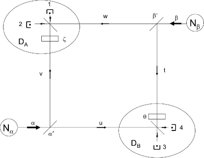
Figure 1: Two Fock states, with populations $N_{\alpha}$ and $N_{\beta}$, enter beam splitters, and are then made to interfere in two different regions of space $D_{A}$ and $D_{B}$, with detectors 1 and 2 in the former, 3 and 4 in the latter. The number of particles $m_{j}$ in each of the channels $j=1,2,3,4$ are counted.

We now calculate the probability of any sequence of results with the same approach as in [48]. This provides correct results if one assumes that the experiment is perfect; a more elaborate approach is necessary to study the effects of experimental imperfections, and will be given in § 2.

1.1 Probabilities of the various results

We consider spinless particles and we assume that the initial state is:

$$\left|\Phi_{0}\right\rangle=\left|N_{\alpha},N_{\beta}\right\rangle\equiv~{}\frac{1}{\sqrt{N_{\alpha}!N_{\beta}!}}~{}\left[\left(a_{\alpha}\right)^{\dagger}\right]^{N_{\alpha}}\left[\left(a_{\beta}\right)^{\dagger}\right]^{N_{\beta}}\left|0\right\rangle$$ (1)

where $\left|0\right\rangle$ is the vacuum state; single particle state $\alpha$ corresponds to that populated by the first source, $\beta$ to that populated by the second source. The destruction operators $a_{1}\cdots a_{4}$ of the output modes can be written in terms of those of the modes at the sources $a_{\alpha},$ $a_{\beta},$ $a_{\alpha^{\prime}}$ and $a_{\beta^{\prime}}$ (including the vacuum input modes, $a_{\alpha^{\prime}}$ and $a_{\beta^{\prime}}$, which are included to maintain unitarity) by tracing back from the detectors to the sources, providing a phase shift of $\pi/2$ at each reflection and $\zeta$ or $\theta$ at the shifters, and a $1/\sqrt{2}$ for normalization at each beam splitter. Thus we find:

$$\left(\begin{array}[c]{l}a_{1}\\ a_{2}\\ a_{3}\\ a_{4}\end{array}\right)=\frac{1}{2}\left(\begin{array}[c]{llll}ie^{i\zeta}&e^{i\zeta}&i&-1\\ -e^{i\zeta}&ie^{i\zeta}&1&i\\ i&-1&ie^{i\theta}&e^{i\theta}\\ 1&i&-e^{i\theta}&e^{i\theta}\end{array}\right)\left(\begin{array}[c]{l}a_{\alpha}\\ a_{\alpha^{\prime}}\\ a_{\beta}\\ a_{\beta^{\prime}}\end{array}\right)$$ (2)

Since $a_{\alpha^{\prime}}$ and $a_{\beta^{\prime}}$ do not contribute we can write simply:

$$\begin{array}[c]{l}a_{1}=\frac{1}{2}\left[ie^{i\zeta}a_{\alpha}+ia_{\beta}\right]\\ a_{2}=\frac{1}{2}\left[-e^{i\zeta}a_{\alpha}+a_{\beta}\right]\\ a_{3}=\frac{1}{2}\left[ia_{\alpha}+ie^{i\theta}a_{\beta}\right]\\ a_{4}=\frac{1}{2}\left[a_{\alpha}-e^{i\theta}a_{\beta}\right]\end{array}$$ (3)

In short, we write these expressions as:

$$a_{j}=v_{j\alpha}a_{\alpha}+v_{j\beta}a_{\beta}.$$ (4)

We suppose that Alice finds $m_{1}$ positive results and $m_{2}$ negative results for a total of $m_{A}$ measurements; Bob finds $m_{3}$ positive and $m_{4}$ negative results in his $m_{B}$ total measurements. The quantum probability of this series of results is the squared modulus of the scalar product of state $\left|\Phi_{0}\right\rangle$ by the state associated with the measurement:

$$\mathcal{P(}m_{1},m_{2},m_{3},m_{4})=\frac{1}{m_{1}!m_{2}!m_{3}!m_{4}!}~{}\left|\left\langle 0\right|\left(a_{1}\right)^{m_{1}}\cdots\left(a_{4}\right)^{m_{4}}\left|N_{\alpha},N_{\beta}\right\rangle\right|^{2}$$ (5)

where the matrix element is non-zero only if:

$$m_{1}+m_{2}+m_{3}+m_{4}=N_{\alpha}+N_{\beta}=N$$ (6)

We can calculate this matrix element by substituting (1) and (4) and expanding in binomial series:

$$\begin{array}[c]{l}\displaystyle\left\langle 0\right|\left(a_{1}\right)^{m_{1}}\cdots\left(a_{1}\right)^{m_{4}}\left|N_{\alpha},N_{\beta}\right\rangle=\frac{1}{\sqrt{N_{\alpha}!N_{\beta}!}}\left\langle 0\right|\prod_{j=1}^{4}\left(v_{j\alpha}a_{\alpha}+v_{j\beta}a_{\beta}\right)^{m_{j}}\left(a_{\alpha}^{\dagger}\right)^{N_{\alpha}}\left(a_{\beta}^{\dagger}\right)^{N_{\beta}}\left|0\right\rangle\\ \lx@intercol\hfil\displaystyle=\frac{1}{\sqrt{N_{\alpha}!N_{\beta}!}}\sum_{p_{\alpha 1}=0}^{m_{1}}\frac{m_{1}!}{p_{\alpha 1}!p_{\beta 1}!}\left(v_{1\alpha}\right)^{p_{\alpha 1}}\left(v_{1\beta}\right)^{p_{\beta 1}}...\hfil\lx@intercol\\ \lx@intercol\hfil\displaystyle..\sum_{p_{\alpha 4}=0}^{m_{4}}\frac{m_{4}!}{p_{\alpha 4}!p_{\beta 4}!}\left(v_{4\alpha}\right)^{p_{\alpha 4}}\left(v_{4\beta}\right)^{p_{\beta 4}}~{}\left\langle 0\right|\left(a_{\alpha}\right)^{p_{\alpha 1}+\cdots+p_{\alpha 4}}\left(a_{\beta}\right)^{p_{\beta 1}+\cdots+p_{\beta 4}m_{i}}\left(a_{\alpha}^{\dagger}\right)^{N_{\alpha}}\left(a_{\beta}^{\dagger}\right)^{N_{\beta}}\left|0\right\rangle\lx@intercol\end{array}$$ (7)

where $p_{\beta j}=m_{j}-p_{\alpha j}$ for any $j$. The matrix element at the end of this expression is:

$$N_{\alpha}!N_{\beta}!~{}\delta_{N_{\alpha},~{}p_{\alpha 1}+\cdots+~{}p_{\alpha 4}}~{}\delta_{N_{\beta},~{}p_{\beta 1}+\cdots~{}+p_{\beta 4}}$$ (8)

But by definition the sum of all $p$’s is equal to $m_{1}+m_{2}+m_{3}+m_{4}$ which, according to (6), is $N_{\alpha}+N_{\beta}$; the two Kronecker delta’s in (8) are therefore redundant. For the matrix element to be non zero and equal to $N_{\alpha}!N_{\beta}!$, it is sufficient that the difference between the sums $p_{\alpha 1}+\cdots+~{}p_{\alpha 4}$ and $p_{\beta 1}+\cdots~{}+p_{\beta 4}$ be equal to $N_{\alpha}-N_{\beta}$, a condition which we can express through the integral:

$$\int_{-\pi}^{\pi}\frac{d\mu}{2\pi}e^{i(N_{\beta}-N_{\alpha}+p_{\alpha 1}+\cdots+~{}p_{\alpha 4}-p_{\beta 1}+\cdots~{}-p_{\beta 4})\mu}=\delta_{N_{\alpha}-N_{\beta},~{}p_{\alpha 1}+\cdots+~{}p_{\alpha 4}-p_{\beta 1}-\cdots~{}-p_{\beta 4}}$$ (9)

When this is inserted into (7), in the second line every $v_{j\alpha}$ becomes $v_{j\alpha}e^{i\mu}$, every $v_{j\beta}$ becomes $v_{j\beta}e^{-i\mu}$, and we can redo the sums and write the probability amplitude as:

$$\sqrt{N_{\alpha}!N_{\beta}!}\int_{-\pi}^{\pi}\frac{d\mu}{2\pi}e^{{}^{i\left(N_{\beta}-N_{\alpha}\right)\mu}}\prod_{j=1}^{4}\left(v_{j\alpha}e^{i\mu}+v_{j\beta}e^{-i\mu}\right)^{m_{j}}$$ (10)

Thus the probability is:

$$\mathcal{P(}m_{1},m_{2},m_{3},m_{4})=\frac{N_{\alpha}!N_{\beta}!}{m_{1}!m_{2}!m_{3}!m_{4}!}\int_{-\pi}^{\pi}\frac{d\mu}{2\pi}\int_{\pi}^{\pi}\frac{d\mu^{\prime}}{2\pi}~{}~{}e^{{}^{i\left(N_{\beta}-N_{\alpha}\right)\left(\mu-\mu^{\prime}\right)}}\prod_{j=1}^{4}\left[\Omega_{j}^{\ast}(\mu^{\prime})\Omega_{j}(\mu)\right]^{m_{i}}$$ (11)

with:

$$\Omega_{j}(\mu)=v_{j\alpha}e^{i\mu}+v_{j\beta}e^{-i\mu}$$ (12)

Each of the factors $\Omega_{j}^{\ast}(\mu^{\prime})\Omega_{j}(\mu)$ can now be simplified according to:

$$\Omega_{j}^{\ast}(\mu^{\prime})\Omega_{j}(\mu)=\left|v_{j\alpha}\right|^{2}e^{i\left(\mu-\mu^{\prime}\right)}+\left|v_{j\beta}\right|^{2}e^{i\left(\mu^{\prime}-\mu\right)}+v_{j\alpha}^{\ast}v_{j\beta}~{}e^{-i\left(\mu+\mu^{\prime}\right)}+v_{j\alpha}v_{j\beta}^{\ast}~{}e^{i\left(\mu+\mu^{\prime}\right)}$$ (13)

which, when (3) is inserted, gives:

$$\frac{1}{2}\left[\cos\left(\mu-\mu^{\prime}\right)\pm\cos\left(\zeta+\mu+\mu^{\prime}\right)\right]~{}~{}~{}~{}~{}\text{or}~{}~{}~{}~{}~{}\frac{1}{2}\left[\cos\left(\mu-\mu^{\prime}\right)\pm\cos\left(-\theta+\mu+\mu^{\prime}\right)\right]$$

depending on the value of $j$. Now, if we define:

$$\begin{array}[c]{l}\lambda=\mu+\mu^{\prime}\\ \Lambda=\mu-\mu^{\prime}\end{array}$$ (14)

we finally obtain:

$$\begin{array}[c]{l}\displaystyle\mathcal{P(}m_{1},m_{2},m_{3},m_{4})=\frac{N_{\alpha}!N_{\beta}!}{m_{1}!m_{2}!m_{3}!m_{4}!}~{}2^{-N}\int_{-\pi}^{\pi}\frac{d\lambda}{2\pi}\int_{-\pi}^{\pi}\frac{d\Lambda}{2\pi}\cos\left[(N_{\beta}-N_{\alpha})\Lambda\right]\\ \lx@intercol\hfil\displaystyle\times\left[\cos\Lambda+\cos\left(\zeta+\lambda\right)\right]^{m_{1}}\left[\cos\Lambda-\cos\left(\zeta+\lambda\right)\right]^{m_{2}}\left[\cos\Lambda+\cos\left(\theta-\lambda\right)\right]^{m_{3}}\left[\cos\Lambda-\cos\left(\theta-\lambda\right)\right]^{m_{4}}\lx@intercol\end{array}$$ (15)

where we have used $\Lambda$ parity to reduce $e^{i\left(N_{\beta}-N_{\alpha}\right)\Lambda}$ to a cosine.

1.2 Effects of particle losses

We now study cases where losses occur in the experiment; some particles emitted by the sources are missed by the detectors sitting at the four output ports. The total number of particles they detect is $M$, with $M\leq N$; an analogous situation was already considered in the context of spin measurements [16, 17]. We first focus on losses taking place near the sources of particles, then on those in the detection regions.

1.2.1 Losses at the sources

As a first simple model for treating losses, we consider the experimental configuration shown in Fig. 2, where additional beam splitters divert some particles before they reach the input of the interferometer. If $T$ and $R$ are the transmission and the reflection coefficients of the additional beam splitters, with:

$$R+T=1$$ (16)

the unitary transformations become:

$$\begin{array}[c]{l}a_{1}=\frac{i\sqrt{T}}{2}\left[e^{i\zeta}a_{\alpha}+\alpha_{\beta}\right]\\ a_{2}=\frac{\sqrt{T}}{2}\left[-e^{i\zeta}a_{\alpha}+\alpha_{\beta}\right]\\ a_{3}=\frac{i\sqrt{T}}{2}\left[a_{\alpha}+e^{i\theta}a_{\beta}\right]\\ a_{4}=\frac{\sqrt{T}}{2}\left[a_{\alpha}-e^{i\theta}a_{\beta}\right]\\ a_{5}=i\sqrt{R}\left[a_{\alpha}\right]\\ a_{6}=i\sqrt{R}\left[a_{\beta}\right]\end{array}$$ (17)

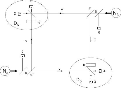
Figure 2: The experiment is the same as in figure 1, but now we assume that two beam splitters are inserted between the two sources and the inputs of the interferometer. Then, the total number of particles $M$ measured at the output of the interferometer may be less than $N$.

The probability amplitude associated with a series of results $m_{1}$, …$m_{5}$, $m_{6}$ is now:

$$\frac{\left\langle 0\right|\left(a_{1}\right)^{m_{1}}\cdots\left(a_{4}\right)^{m_{4}}\left(a_{5}\right)^{m_{5}}\left(a_{6}\right)^{m_{6}}\left|N_{\alpha},N_{\beta}\right\rangle}{\sqrt{m_{1}!....m_{5}!~{}m_{6}!}}$$ (18)

or, taking into account the last two equations (17):

$$R^{{}^{\left(m_{5}+m_{6}\right)/2}}\sqrt{\frac{N_{\alpha}!}{\left(N_{\alpha}-m_{5}\right)!~{}m_{5}!}\times\frac{N_{\beta}!}{\left(N_{\beta}-m_{6}\right)!~{}m_{6}!}}\frac{\left\langle 0\right|\left(a_{1}\right)^{m_{1}}\cdots\left(a_{4}\right)^{m_{4}}\left|N_{\alpha}-m_{5},N_{\beta}-m_{6}\right\rangle}{\sqrt{m_{1}!...m_{4}!}}$$ (19)

The fraction on the right of this expression can be obtained from the calculations of § 1.1, by just replacing $N_{\alpha}$ by $N_{\alpha}-m_{5}$, $N_{\beta}$ by $N_{\beta}-m_{6}$ in (10). With this substitution, the numerical factor in front of that expression combines with that of (19) to give a prefactor:

$$R^{{}^{\left(m_{5}+m_{6}\right)/2}}\sqrt{\frac{N_{\alpha}!N_{\beta}!}{m_{5}!m_{6}!}}$$ (20)

The next step is to sum the probabilities over $m_{5}$ and $m_{6}$, keeping the four $m_{1}$, ..$m_{4}$ constant; we vary $m_{5}$ and $m_{6}$ with a constant sum $N-M$, where $M$ is defined as:

$$M=m_{1}+m_{2}+m_{3}+m_{4}\leq N$$ (21)

The $\cos\left[\left(N_{\beta}-N_{\alpha}\right)\Lambda\right]$ inside the integral of (15) arose from an exponential $e^{i\left[\left(N_{\beta}-N_{\alpha}\right)\Lambda\right]}$, which now becomes:

$$e^{i\left(N_{\beta}-N_{\alpha}+m_{5}-m_{6}\right)\Lambda}$$ (22)

so that the summation over $m_{5}$ and $m_{6}$ reconstructs a power of a binomial:

$$\frac{1}{\left(N-M\right)!}\left[e^{i\Lambda}+e^{-i\Lambda}\right]^{N-M}=\frac{2^{(N-M)}}{\left(N-M\right)!}\left[\cos\Lambda\right]^{N-M}$$ (23)

When the powers of $R$ and $T$ are included as well as the factors $2^{-M}$ and $2^{(N-M)}$, equation (15) is now replaced by:

$$\begin{array}[c]{l}\displaystyle\mathcal{P}_{M}\mathcal{(}m_{1},m_{2},m_{3},m_{4})=\frac{N_{\alpha}!N_{\beta}!}{m_{1}!m_{2}!m_{3}!m_{4}!}2^{N-2M}\frac{T^{M}~{}R^{N-M}~{}}{\left(N-M\right)!}\int_{-\pi}^{\pi}\frac{d\lambda}{2\pi}\int_{-\pi}^{\pi}\frac{d\Lambda}{2\pi}\cos\left[(N_{\beta}-N_{\alpha})\Lambda\right]~{}\left[\cos\Lambda\right]^{N-M}\\ \lx@intercol\hfil\displaystyle\times\left[\cos\Lambda+\cos\left(\zeta+\lambda\right)\right]^{m_{1}}\left[\cos\Lambda-\cos\left(\zeta+\lambda\right)\right]^{m_{2}}\lx@intercol\\ \lx@intercol\hfil\displaystyle\times\left[\cos\Lambda+\cos\left(\theta-\lambda\right)\right]^{m_{3}}\left[\cos\Lambda-\cos\left(\theta-\lambda\right)\right]^{m_{4}}\lx@intercol\end{array}$$ (24)

where $M$ is defined in (21). This result is similar to (15), but includes a power of $\cos\Lambda$ inside the integral, which we will discuss in § 1.3. We note that this power of $\cos\Lambda$ introduces exactly the same factor as that already obtained in [16], in the context of spin condensates and particles missed in transverse spin measurements.

If $T=1$ and $R=0$, expression (24) vanishes unless $M$ has its maximal value $M=N$; then expression (15) is recovered, as expected. If $R$ and $T$ have intermediate values, $M$ has a probability distribution including any value less than $N$, with of course smaller values favored when $T$ is small and $R$ large.

1.2.2 Losses at the detectors

Instead of inserting additional beam splitters just after the sources, we can put them just before the detectors, as in Fig. 3; this provides a model for losses corresponding to imperfect detectors with quantum efficiencies less than $100\%$.

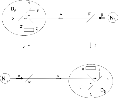
Figure 3: The experiment is the same as that in figure 2, but now 4 beam splitters are inserted just before the 4 particle detectors, which sit in channels $1$,$2$,$3$,$4$; the other channels, $1^{\prime}$, $2^{\prime}$, $3^{\prime}$, $4^{\prime}$ contain no detector. This provides a model for calculating the effect of limited quantum efficiencies of the detectors.

Instead of 6 destruction operators as in (17), we now have 8; each operator $a_{j}$ ($j=1,2,3,4)$ corresponding to one of the 4 the detectors is now associated with a second operator $a_{j}^{\prime}$ corresponding to the other output port with no detector. For instance, for $j=1$, one has:

$$a_{1}=\frac{i\sqrt{T}}{2}\left[e^{i\zeta}a_{\alpha}+\alpha_{\beta}\right]\text{ \ \ \ \ \ \ ; \ \ \ \ \ \ \ \ }a_{1}^{\prime}=\frac{-\sqrt{R}}{2}\left[e^{i\zeta}a_{\alpha}+\alpha_{\beta}\right]$$ (25)

and similar results for $j=2$,$3$,$4$. The calculation of the probability associated with results $m_{1}$,..$m_{4}$ (with their sum equal to $M$) and $m_{1}^{\prime}$, ..$m_{4}^{\prime}$ (with their sum equal to $N-M$) is very similar to that of § 1.1; formula (5) becomes:

$$\mathcal{P(}m_{1},..m_{4};m_{1}^{\prime},..m_{4}^{\prime})=\frac{1}{m_{1}!..!m_{4}!\times m_{1}^{\prime}!..!m_{4}^{\prime}!}~{}\left|\left\langle 0\right|\left(a_{1}\right)^{m_{1}}\cdots\left(a_{4}\right)^{m_{4}}\times\left(a_{1}^{\prime}\right)^{m_{1}^{\prime}}\cdots\left(a_{4}^{\prime}\right)^{m_{4}^{\prime}}\left|N_{\alpha},N_{\beta}\right\rangle\right|^{2}$$

Since $a_{j}$ and $a_{j}^{\prime}$ are almost the same operator (they just differ by a coefficient), the result is still given by the right hand side of (15), with the following changes:

(i) each $m_{j}$ is now replaced by the sum $m_{j}+m_{j}^{\prime}$

(ii) $m_{1}!..!m_{4}!$ in the denominator is multiplied by $m_{1}^{\prime}!..!m_{4}^{\prime}!$

(ii) a factor $T^{M}\times R^{N-M}$ appears in front of the expression.

Now, we consider the observed results $m_{1}$,..$m_{4}$ as fixed, and add the probabilities associated with all possible non-observed values $m_{1}^{\prime}$, ..$m_{4}^{\prime}$; this amounts to distributing $N-M$ unobserved particles in any possible way among all output channels without detectors. The summation is made in two steps:

(i) summations over $m_{1}^{\prime}$ and $m_{2}^{\prime}$ at constant sum $m_{1}^{\prime}+m_{2}^{\prime}=m_{A}^{\prime}$, and over $m_{3}^{\prime}$ and $m_{4}^{\prime}$ at constant sum $m_{3}^{\prime}+m_{4}^{\prime}=m_{B}^{\prime}$

(ii) summation over $m_{A}^{\prime}$ and $m_{B}^{\prime}$ at constant sum $m_{A}^{\prime}+m_{B}^{\prime}=N-M$

The first summation provides:

$$\sum_{m_{1}^{\prime}+m_{2}^{\prime}=m_{A}^{\prime}}\frac{1}{m_{1}^{\prime}!m_{2}^{\prime}!}\left[\cos\Lambda+\cos\left(\zeta+\lambda\right)\right]^{m_{1}^{\prime}}\left[\cos\Lambda-\cos\left(\zeta+\lambda\right)\right]^{m_{2}^{\prime}}=\frac{1}{m_{A}^{\prime}!}\left[2\cos\Lambda\right]^{m_{A}^{\prime}}$$ (26)

and similarly for the summation over $m_{3}^{\prime}$ and $m_{4}^{\prime}$. Then the last summation provides:

$$\sum_{m_{A}^{\prime}+m_{B}^{\prime}=N-M}\frac{1}{m_{A}^{\prime}!m_{B}^{\prime}!}\left[2\cos\Lambda\right]^{m_{A}^{\prime}}\left[2\cos\Lambda\right]^{m_{B}^{\prime}}=\frac{1}{N-M!}\left[4\cos\Lambda\right]^{N-M}$$ (27)

At the end, as in § 1.2.1, we see that each unobserved particle introduces a factor $\cos\Lambda$ so that, in the integral giving the probability, a factor $\left[\cos\Lambda\right]^{N-M}$ appears; actually, we end up with an expression that is again exactly (24). The presence of this factor inside the integral seems to be a robust property of the effects of imperfect measurements (for brevity, we do not prove the generality of this statement, for instance by studying the effect of additional beam splitters that are inserted elsewhere, for instance in other parts of the interferometer).

1.3 Discussion

The discussion of the physical content of equation (15) and (24) is somewhat similar to that for spin measurements [16]. One difference is that, here, we consider that the total number of measurements $m_{A}=m_{1}+m_{2}$ made by Alice, as well as the total number of measurements $m_{B}=m_{3}+m_{4}$ made by Bob, are left to fluctuate with a constant sum $M$; the particles emitted by the sources may localize in any of the four detection regions. With spins, the numbers of detections depends on the number of spin apparatuses used by Alice and Bob, so that it was more natural to assume that $m_{A}$ and $m_{B}$ are fixed. This changes the normalization and the probabilities, but not the dependence on the experimental parameters, which is given by (15) and (24). A discussion of the normalization integrals is given in the Appendix.

1.3.1 Effects of $N_{\alpha}$, $N_{\beta}$ and of the number of measurements

If the numbers of particles in the sources are different  ($N_{\alpha}\neq N_{\beta}$), a term in $\cos\left[(N_{\beta}-N_{\alpha})\Lambda\right]$ appears in both equations; let us assume for simplicity that all $N$ particles are measured $(M=N)$, so that equation (15) applies, and for instance that $N_{\alpha}>N_{\beta}$. Then, in the product of factors inside the integral, only some terms can provide a non-zero contribution after integration over $\Lambda$; we must choose at least $N_{\alpha}-N_{\beta}$ factors contributing through $\cos\left(\Lambda\right)$, and thus at most $N-(N_{\alpha}-N_{\beta})=2N_{\beta}$ factors contributing through the $\theta$ dependent terms. Therefore $2N_{\beta}$ is the maximum number of particles providing results that depends on the settings of the interferometer; all the others have equal probabilities $1/2$, whatever the phase shift is. This is physically understandable, since $(N_{\alpha}-N_{\beta})$ particles from the first source unmatched particles from the other, and can thus not contribute to an interference effect. All particles can contribute coherently to the interference only if $N_{\alpha}=N_{\beta}$.

If the numbers of particles in the sources are equal ($N_{\alpha}=N_{\beta}$), the sources are optimal; equation (24) contains the effect of missing some particles in the measurements. If the number of experiments $M$ is much less than a very large $N$, because $\cos\Lambda^{N-M}$ peaks up sharply at $\Lambda=0$, the result simplifies into:

$$\mathcal{P}_{M}\mathcal{(}m_{1},m_{2},m_{3},m_{4})\sim\frac{1}{m_{1}!m_{2}!m_{3}!m_{4}!}\int_{-\pi}^{\pi}\frac{d\lambda}{2\pi}~{}~{}\left[1+\cos\left(\zeta+\lambda\right)\right]^{m_{1}}\left[1-\cos\left(\zeta+\lambda\right)\right]^{m_{2}}$$

$$\times\left[1+\cos\left(\theta-\lambda\right)\right]^{m_{3}}\left[1-\cos\left(\theta-\lambda\right)\right]^{m_{4}}$$ (28)

We then recover “classical” results, similar to those of refs. [29] or [49]. Suppose that we introduce a classical phase $\lambda$ and calculate classically the interference effects at both beam splitters. This leads to intensities proportional to $\left[1+\cos\left(\zeta+\lambda\right)\right]$ and $\left[1-\cos\left(\zeta+\lambda\right)\right]$ on both sides of the interferometer in $D_{A}$, and similar results for $D_{B}$. Now, if we assume that each particle reaching the beam splitter has crossing and reflecting probabilities that are proportional to these intensities (we treat each of these individual processes as independent), and if we consider that this classical phase is completely unknown, an average over $2\pi$ then reconstructs exactly (28). In this case, the classical image of a pre-existing phase leads to predictions that are the same as those of quantum mechanics; this phase will take a completely random value for each realization of the experiment, with for instance no way to force it to take related values in two successive runs. All this fits well within the concept of the Anderson phase, originating from spontaneous symmetry breaking at the phase transition (Bose-Einstein condensation): at this transition point, the quantum system “chooses” a phase, which takes a completely random value, and then plays the role of a classical variable (in the limit of very large systems).

On the other hand, if $N-M$ vanishes, the peaking effect of $\cos\Lambda^{N-M}$ does not occur anymore, $\Lambda$ can take values close to $\pi/2$ , so that the terms in the product inside the integral are no longer necessarily positive; an interpretation in terms of classical probabilities then becomes impossible. In these cases, the phase does not behave as a semi-classical variable, but retains a strong quantum character; the variable $\Lambda$ controls the amount of quantum effects. It is therefore natural to call $\Lambda$ the “quantum angle” and $\lambda$ the “classical phase”.

One could object that, if expression (15) contains negative factors, this does not prove that the same probabilities $\mathcal{P}$ can not be obtained with another mathematical expression without negative probabilities. To show that this is indeed impossible, we have to resort to a more general theorem, the Bell/BCHSH theorem, which proves it in a completely general way; this is what we do in § 3.

1.3.2 Perfect correlations

We now show that, if $N_{\alpha}$ and $N_{\beta}$ are equal and if the number of measurements is maximal ($M=N$), when Alice and Bob choose opposite phase shifts ($\theta=-\zeta$) they always measure the same parity. In this case, the integrand of (15) becomes:

$$\left[\cos\Lambda+\cos\left(\lambda+\zeta\right)\right]^{m_{1}+m_{3}}\left[\cos\Lambda-\cos\left(\lambda+\zeta\right)\right]^{m_{2+}m_{4}}$$ (29)

which can also be written as:

$$2^{N}\left[\sin(\lambda^{\prime}+\frac{\zeta}{2})\right]^{m_{1}+m_{3}}\left[\sin(\lambda^{\prime\prime}-\frac{\zeta}{2})\right]^{m_{1}+m_{3}}\left[\cos(\lambda^{\prime}+\frac{\zeta}{2})\right]^{m_{2}+m_{4}}\left[\cos(\lambda^{\prime\prime}-\frac{\zeta}{2})\right]^{m_{2}+m_{4}}$$ (30)

with the following change of integration variables:

$$\begin{array}[c]{cc}\lambda^{\prime}=\frac{\lambda+\Lambda}{2}&\lambda^{\prime\prime}=\frac{\Lambda-\lambda}{2}\end{array}$$ (31)

If, for instance, $m_{1}+m_{3}$ is odd, instead of $\lambda^{\prime}$ one can take $(\lambda^{\prime}+\zeta/2)$ as an integration variable, and one can see that the integral vanishes because its periodicity - the same is true of course for the $\lambda^{\prime\prime}$ integration, which also vanishes. Similarly, if $m_{2}+m_{4}$ is odd, one can take $(\lambda^{\prime}-\frac{\zeta}{2})$ and $(\lambda^{\prime\prime}-\frac{\zeta}{2})$ as integration variables, and the result vanishes again. Finally, the probability is non-zero only if both $m_{1}+m_{3}$ and $m_{2}+m_{4}$ are even; the conclusion is that Alice and Bob always observe the same parity for their results. This perfect correlation is useful for applying the EPR reasoning to parities.

2 A more elaborate calculation

The advantage of measuring the positions of particles after a beam splitter, that is interference effects providing dichotomic results, is that one has a device that is close to quantum non-demolition experiments. With a resonant laser, one can make an atom fluoresce and emit many photons, without transferring the atom from one arm of the interferometer to the other. This is clearly important in experiments where, as we have seen, all the atoms must be detected to obtain quantum non-local effects. On the other hand, it is well know experimentally that a difficulty with interferometry is the alignment of the devices in order to obtain an almost perfect matching of the wave front. We discuss this problem now.

A general assumption behind the calculation of § 1 is that, in each region of space (for instance at the inputs, or at the 4 outputs), only one mode of the field is populated (only one $a^{\dagger}$ operator is introduced per region). The advantage of this approach is its simplicity, but it nevertheless eludes some interesting questions. For instance, suppose that the energies of the particles emerging from each source differ by some arbitrarily small quantity; after crossing all beam splitters, they would reach the detection regions in two orthogonal modes, so that the probability of presence would be the sum of the corresponding probabilities, without any interference term. On the other hand, all interesting effects obtained in [48] are precisely interference effects arising because, in each detection region, there is no way to tell which source emitted the detected particles. Does this mean that these effects disappear as soon as the sources are not strictly identical, so that the quantum interferences will never be observable in practice?

To answer this kind of question, here we will develop a more detailed theory of the detection of many particles in coincidence, somewhat similar to Glauber’s theory of photon coincidences [50]; nevertheless, while in that theory only the initial value of the n-th time derivative was calculated, here we study the whole time dependence of the correlation function. Our result will be that, provided the interferometers and detectors are properly aligned, it is the detection process that restores the interesting quantum effects, even if the sources do not emit perfectly identical wavefronts in the detection regions, as was assumed in the calculations of § 1. As a consequence, the reader who is not interested in experimental limitations may skip this section and proceed directly to § 3.

In this section we change the definition of the single particle states: $\alpha$ now corresponds to a state for which the wave function originates from the first source, is split into two beams when reaching the first beam splitter, and into two beams again when it reaches the beam splitters associated with the regions of measurement $D_{A}$ and $D_{B}$;  the same is true for state $\beta$. In this point of view, all the propagation in the interferometers is already included in the states. We note in passing that the evolution associated with the beam splitters is unitary; the states $\alpha$ and $\beta$ therefore remain perfectly orthogonal, even if they overlap in some regions of space. Having changed the definition of the single particle states, we keep (1) to define the N particle state of the system.

2.1 Pixels as independent detectors

We model the detectors sitting after the beam splitters by assuming that they are the juxtaposition of a large number $\mathcal{Q}$ of independent pixels, which we treat as independent detectors. This does not mean that the positions of the impact of all particles are necessarily registered in the experiment; our calculations still apply if, for instance, only the total number of impact in each channel is recorded. The only thing we assume is that the detection of particles in different points leads to orthogonal states of some part of the apparatus (or the environment), so that we can add the probabilities of the events corresponding to different orthogonal states; whether or not the information differentiating these states is recorded in practice does not matter.

If the number of pixels $\mathcal{Q}$ is very large, the probability of detection of two bosons at the same pixel is negligible. If we note $N=N_{\alpha}+N_{\beta}$, this probability is bounded by:

$$\frac{1}{\mathcal{Q}}+\frac{2}{\mathcal{Q}}+....+\frac{N}{\mathcal{Q}}=\frac{N(N+1)}{2\mathcal{Q}}$$ (32)

so that we will assume that:

$$\mathcal{Q}\gg N^{2}$$ (33)

Moreover, we consider events where all $N$ particles are detected (the probabilities of events where some particles are missed can be obtained from the probabilities of these events in a second step, as in [16]).

2.2 Flux of probability at the pixels in a stationary state

Each pixel $j$ is considered as defining a region of space $\Delta_{j}$ in which the particles are converted into a macroscopic electric current, as in a photomultiplier. The particles enter this region through the front surface $S_{j}$ of the pixel; all particles crossing $S_{j}$ disappear in a conversion process that is assumed to have 100% efficiency. What we need, then, is to calculate the flux of particles entering the front surfaces of the pixels. It is convenient to reason in the $3N$ dimension configuration space, in which the hyper-volume associated with the $N$ different pixels is:

$$V_{N}=\Delta_{1}\otimes\Delta_{2}\otimes\Delta_{3}....\otimes\Delta_{N}$$ (34)

which has an front surface given by:

$$S_{N}=S_{1}\otimes\Delta_{2}\otimes\Delta_{3}....\otimes\Delta_{N}~{}+~{}\Delta_{1}\otimes S_{2}\otimes\Delta_{3}....\otimes\Delta_{N}+~{}..+~{}~{}\Delta_{1}\otimes\Delta_{2}\otimes\Delta_{3}....\otimes S_{N}$$ (35)

The density of probability in this space is defined in terms of the boson field operator $\Psi(\mathbf{r})$ as:

$$\rho_{N}(\mathbf{r}_{1},\mathbf{r}_{2},...,\mathbf{r}_{N})=\Psi^{\dagger}(\mathbf{r}_{1})\Psi(\mathbf{r}_{1})~{}\Psi^{\dagger}(\mathbf{r}_{2})\Psi(\mathbf{r}_{2})~{}...~{}\Psi^{\dagger}(\mathbf{r}_{N})\Psi(\mathbf{r}_{N})$$ (36)

where we assume that all $\mathbf{r}_{j}$’s are different (all pixels are disjoint). The components of the $3N$ dimension current operator $\mathbf{J}_{N}$ are:

$$\mathbf{J}_{N}=\left\{\begin{array}[c]{l}\frac{\hbar}{2mi}\left[\Psi^{\dagger}(\mathbf{r}_{1})\mathbf{\nabla}\Psi(\mathbf{r}_{1})-\mathbf{\nabla}\Psi^{\dagger}(\mathbf{r}_{1})\Psi(\mathbf{r}_{1})\right]~{}~{}\Psi^{\dagger}(\mathbf{r}_{2})\Psi(\mathbf{r}_{2})~{}...\Psi^{\dagger}(\mathbf{r}_{N})\Psi(\mathbf{r}_{N})+\\ +\frac{\hbar}{2mi}\Psi^{\dagger}(\mathbf{r}_{1})\Psi(\mathbf{r}_{1})~{}\left[\Psi^{\dagger}(\mathbf{r}_{2})\mathbf{\nabla}\Psi(\mathbf{r}_{2})-\mathbf{\nabla}\Psi^{\dagger}(\mathbf{r}_{2})\Psi(\mathbf{r}_{2})\right]...\Psi^{\dagger}(\mathbf{r}_{N})\Psi(\mathbf{r}_{N})+\\ +...\\ +\frac{\hbar}{2mi}\Psi^{\dagger}(\mathbf{r}_{1})\Psi(\mathbf{r}_{1})~{}\Psi^{\dagger}(\mathbf{r}_{2})\Psi(\mathbf{r}_{2})~{}...\left[\Psi^{\dagger}(\mathbf{r}_{N})\mathbf{\nabla}\Psi(\mathbf{r}_{N})-\mathbf{\nabla}\Psi^{\dagger}(\mathbf{r}_{N})\Psi(\mathbf{r}_{N})\right]\end{array}\right.$$ (37)

In the Heisenberg picture, the quantum operator $\rho_{N}$ obeys the evolution equation:

$$\frac{d}{dt}\rho_{N}(\mathbf{r}_{1},\mathbf{r}_{2},...,\mathbf{r}_{N};t)+\mathbf{\nabla}_{N}\cdot\mathbf{J}_{N}=0$$ (38)

where $\mathbf{\nabla}_{N}$ is the $N$ dimensional divergence. The flux of probability entering the $3N$ dimension volume $S_{N}$ it then:

$$\begin{array}[c]{l}\mathcal{F}(\Delta_{1},\Delta_{2},...\Delta_{N})~{}=~{}<\Phi_{0}\mid F\left(\Delta_{1}\right)\times G\left(\Delta_{2}\right)\times....G\left(\Delta_{N}\right)\mid\Phi_{0}>\\ \lx@intercol\hfil+~{}<\Phi_{0}\mid G\left(\Delta_{1}\right)\times F\left(\Delta_{2}\right)\times....G\left(\Delta_{N}\right)\mid\Phi_{0}>+...\lx@intercol\\ \lx@intercol\hfil+~{}<\Phi_{0}\mid G\left(\Delta_{1}\right)\times G\left(\Delta_{2}\right)\times....F\left(\Delta_{N}\right)\mid\Phi_{0}>\lx@intercol\end{array}$$ (39)

where $F(\Delta_{j})$ is the operator defined as a flux surface integral associated to pixel $j$:

$$F\left(\Delta_{j}\right)=\frac{\hbar}{2mi}~{}\int_{S_{j}}d^{2}\mathbf{s\cdot}~{}\left[\Psi^{\dagger}(\mathbf{r}^{{}^{\prime}})\mathbf{\nabla}\Psi(\mathbf{r}^{{}^{\prime}})-\mathbf{\nabla}\Psi^{\dagger}(\mathbf{r}^{{}^{\prime}})\Psi(\mathbf{r}^{{}^{\prime}})\right]$$ (40)

($d^{2}\mathbf{s}$ the differential vector perpendicular to the surface) and where $G(\Delta_{j})$ is a volume integral associated to the same pixel:

$$G\left(\Delta_{j}\right)=\int_{\Delta_{j}}d^{3}r^{\prime}~{}\Psi^{\dagger}(\mathbf{r}^{{}^{\prime}})\Psi(\mathbf{r}^{{}^{\prime}})$$ (41)

The value of $\mathcal{F}(\Delta_{1},\Delta_{2},...\Delta_{N})$ provides the time derivative of the probability of detection at all selected pixels, which we calculate in § 2.4.

Now, because the various pixels do not overlap, the field operators commute and we can push all $\Psi^{\dagger}$’s to the left, all $\Psi$’s to the right; then we expand these operators on a basis that has $u_{\alpha}$ and $u_{\beta}$ as its two first vectors:

$$\Psi(\mathbf{r})=u_{\alpha}(\mathbf{r})~{}a_{\alpha}~{}+u_{\beta}(\mathbf{r})~{}a_{\beta}+...~{}$$ (42)

The end of the expansion, noted $....$, corresponds to the components of $\Psi(\mathbf{r})$ on other modes that must be added to modes $\alpha$ and $\beta$ to form a complete orthogonal basis in the space of states of one single particle; it is easy to see that they give vanishing contributions to the average in state $\mid\Phi_{0}>$. The structure of any term in (39) then becomes (for the sake of simplicity, we just write the first term):

$$\begin{array}[c]{l}<\Phi_{0}\mid\mathcal{O}_{a,a\dagger}~{}~{}\frac{\hbar}{2mi}\left\{\int_{\Delta_{1}}\left[u_{\alpha}^{\ast}(\mathbf{r}_{1}^{\prime})a_{\alpha}^{\dagger}+u_{\beta}^{\ast}(\mathbf{r}_{1}^{\prime})a_{\beta}^{\dagger}\right]~{}d^{2}\mathbf{s}_{1}\cdot\left[\mathbf{\nabla}u_{\alpha}(\mathbf{r}_{1}^{\prime})a_{\alpha}+\mathbf{\nabla}u_{\beta}(\mathbf{r}_{1}^{\prime})a_{\beta}\right]-\text{c.c.}\right\}\times\\ \lx@intercol\hfil\times{\displaystyle\prod\limits_{j=2}^{N}}\left[u_{\alpha}^{\ast}(\mathbf{r}_{j}^{\prime})a_{\alpha}^{\dagger}+u_{\beta}^{\ast}(\mathbf{r}_{j}^{\prime})a_{\beta}^{\dagger}\right]\left[u_{\alpha}(\mathbf{r}_{j}^{\prime})a_{\alpha}+u_{\beta}(\mathbf{r}_{j}^{\prime})a_{\beta}\right]\mid\Phi_{0}>\lx@intercol\end{array}$$ (43)

where c.c. means complex conjugate and where $\mathcal{O}_{a,a\dagger}$ is the normal ordering operator that puts all the creation operators $a_{\alpha,\beta}^{\dagger}$ to the left of all annihilation operators $a_{\alpha,\beta}$. Each term of the product inside this matrix element contains a product of operators that give, either zero, or always the same matrix element $N_{\alpha}!N_{\beta}!$. For obtaining a non-zero value, two conditions are necessary:

(i) the number of $a_{\alpha}^{\dagger}$’s should be equal to that of $a_{\alpha}$’s

(ii) the number of $a_{\alpha}$’s, minus that of $a_{\beta}$’s, should be equal to $N_{\alpha}-N_{\beta}$.

These conditions are fulfilled with the help of two integrals:

$$\int_{-\pi}^{\pi}\frac{d\lambda}{2\pi}~{}~{}\int_{-\pi}^{\pi}\frac{d\Lambda}{2\pi}~{}~{}e^{i(N_{\beta}-N_{\alpha})\Lambda}$$ (44)

and by multiplying:

(i) every $u_{\alpha}(\mathbf{r}_{j}^{\prime})$ by $e^{i\lambda}$, and every $u_{\alpha}^{\ast}(\mathbf{r}_{j}^{\prime})$ by $e^{-i\lambda}$ (without changing the wave functions related to $\beta$)

(ii) then every $u_{\alpha}(\mathbf{r}_{j}^{\prime})$ by $e^{i\Lambda}$, and every $u_{\beta}(\mathbf{r}_{j}^{\prime})$ by $e^{-i\Lambda}$ (without touching the complex conjugate wave functions).

This provides:

$$\begin{array}[c]{l}\mathcal{F\sim}\int_{-\pi}^{\pi}\frac{d\lambda}{2\pi}~{}~{}\int_{-\pi}^{\pi}\frac{d\Lambda}{2\pi}~{}~{}e^{i(N_{\beta}-N_{\alpha})\Lambda}\\ \frac{\hbar}{2mi}\int_{\Delta_{1}}d^{2}\mathbf{s}_{1}\cdot\left[u_{\alpha}^{\ast}(\mathbf{r}_{1}^{\prime})\mathbf{\nabla}u_{\alpha}(\mathbf{r}_{1}^{\prime})e^{i\Lambda}+u_{\beta}^{\ast}(\mathbf{r}_{1}^{\prime})\mathbf{\nabla}u_{\beta}(\mathbf{r}_{1}^{\prime})e^{-i\Lambda}+u_{\alpha}^{\ast}(\mathbf{r}_{1}^{\prime})\mathbf{\nabla}u_{\beta}(\mathbf{r}_{1}^{\prime})e^{-i(\lambda+\Lambda)}+u_{\beta}^{\ast}(\mathbf{r}_{1}^{\prime})\mathbf{\nabla}u_{\alpha}(\mathbf{r}_{1}^{\prime})e^{i(\lambda+\Lambda)}\right.\\ \lx@intercol\hfil\left.-u_{\alpha}(\mathbf{r}_{1}^{\prime})\mathbf{\nabla}u_{\alpha}^{\ast}(\mathbf{r}_{1}^{\prime})e^{i\Lambda}-u_{\beta}(\mathbf{r}_{1}^{\prime})\mathbf{\nabla}u_{\beta}^{\ast}(\mathbf{r}_{1}^{\prime})e^{-i\Lambda}-u_{\alpha}(\mathbf{r}_{1}^{\prime})\mathbf{\nabla}u_{\beta}^{\ast}(\mathbf{r}_{1}^{\prime})e^{i(\lambda+\Lambda)}-u_{\beta}(\mathbf{r}_{1}^{\prime})\mathbf{\nabla}u_{\alpha}^{\ast}(\mathbf{r}_{1}^{\prime})e^{-i(\lambda+\Lambda)}\right]\lx@intercol\\ \lx@intercol\hfil\times{\displaystyle\prod\limits_{j=2}^{N}}\left[u_{\alpha}^{\ast}(\mathbf{r}_{j}^{\prime})u_{\alpha}(\mathbf{r}_{j}^{\prime})e^{i\Lambda}+u_{\beta}^{\ast}(\mathbf{r}_{j}^{\prime})u_{\beta}(\mathbf{r}_{j}^{\prime})e^{-i\Lambda}+u_{\alpha}^{\ast}(\mathbf{r}_{j}^{\prime})u_{\beta}(\mathbf{r}_{j}^{\prime})e^{-i(\lambda+\Lambda)}+\text{c.c.}\right]~{}+\text{sim.}\lx@intercol\end{array}$$ (45)

where “sim.” is for the $N-1$ similar terms where the gradients occur for $j=2,3,..N$, instead of $j=1$.

Now we assume that the experiment is properly aligned so that the wavefronts of the wave functions $\alpha$ and $\beta$ coincide in all detection regions; then, in the gradients:

$$\mathbf{\nabla}u_{\alpha}(\mathbf{r})=iu_{\alpha}(\mathbf{r})~{}\mathbf{k}_{\alpha}~{}\text{ \ \ \ \ \ \ ; \ \ \ \ \ \ \ }\mathbf{\nabla}u_{\beta}(\mathbf{r})=iu_{\beta}(\mathbf{r})~{}\mathbf{k}_{\beta}~{}$$ (46)

the vectors $\mathbf{k}_{\alpha}$ and $\mathbf{k}_{\beta}$ are parallel; actually, on each pixel $j$ we take these two vectors as equal to the same constant value $\mathbf{k}_{\Delta_{j}}$, assuming that the pixels are small and that the wavelengths of the two wave functions are almost equal. Then (45) simplifies into:

$$\begin{array}[c]{l}\mathcal{F\sim}\int_{-\pi}^{\pi}\frac{d\lambda}{2\pi}~{}~{}\int_{-\pi}^{\pi}\frac{d\Lambda}{2\pi}~{}~{}e^{i(N_{\beta}-N_{\alpha})\Lambda}\frac{\hbar}{2m}\int_{S_{1}}\mathbf{k}_{\Delta_{1}}\cdot d^{2}\mathbf{s}_{1}...\int_{\Delta_{2}}d^{3}r_{2}^{\prime}...\int_{\Delta_{i}}d^{3}r_{i}^{\prime}~{}...\\ \lx@intercol\hfil{\displaystyle\prod\limits_{j=1}^{N}}\left[u_{\alpha}^{\ast}(\mathbf{r}_{j}^{\prime})u_{\alpha}(\mathbf{r}_{j}^{\prime})e^{i\Lambda}+u_{\beta}^{\ast}(\mathbf{r}_{j}^{\prime})u_{\beta}(\mathbf{r}_{j}^{\prime})e^{-i\Lambda}+u_{\alpha}^{\ast}(\mathbf{r}_{j}^{\prime})u_{\beta}(\mathbf{r}_{j}^{\prime})e^{-i(\lambda+\Lambda)}+u_{\beta}^{\ast}(\mathbf{r}_{j}^{\prime})u_{\alpha}(\mathbf{r}_{j}^{\prime})e^{i(\lambda+\Lambda)}\right]~{}+\text{ sim.}\lx@intercol\end{array}$$ (47)

In this expression, the integrand in the $\lambda$ and $\Lambda$ integrals is a product of $N$ factors corresponding to the individual pixels, but this does not imply the absence of correlations (the integral of a product is not the product of integrals). The probability flux $\mathcal{F}$ contains surface integrals through the front surfaces of the pixels, as expected, but also volume integrals in other pixels, which is less intuitive. As a consequence, for obtaining a non-zero probability flux $\mathcal{F}$ in $3N$ dimensions, it is not sufficient to have a non-zero three dimension probability flux through one (or several) pixels; it is also necessary that some probability has already accumulated in the other pixels. In other words, at the very moment where the wave functions reach the front surface of the pixels, the first time derivative of the probability density in $3N$ dimension remains zero, while only the $N$-th order time derivative is non-zero (this will be seen more explicitly in § 2.3). This is analogous to the photon detection process with $N$ atoms in quantum optics, see for instance Glauber [50].

2.3 Time dependence

Consider an experiment where each source emits a wave packet in a finite time. We assume that, in each wave packet, all the particles still remain in the same quantum state, but that this state is now time dependent; the state of the system is then still given by (1), but with time dependent states $\alpha$ and $\beta$, so that the creation operators are now $\left(a_{\alpha}\right)^{\dagger}(t)$ and $\left(a_{\beta}\right)^{\dagger}(t)$. All the calculation of the previous section remains valid, the main difference being that the wave functions are time dependent: $u_{\alpha}(\mathbf{r},t)$ and $u_{\beta}(\mathbf{r},t)$.

We must therefore take into account possible time dependences of the wave fronts of the two wave functions, as well as those of their amplitudes and phases. If, for instance, the interferometer is perfectly symmetric, and if the two wave packets are emitted at the same time, they will reach the beam splitters of the detection regions at the same time with wave fronts that will perfectly overlap at the detectors; the amplitudes of the two wave functions will always be the same. See for instance ref. [51, 52] for a discussion of the time evolution of the phase of Bose-Einstein condensates, including the effects of the interactions within the condensate.

If we consider separately each factor inside the $\lambda$ and $\Lambda$ integral of (47), we come back to the usual three dimension space; two different kinds of integrals then occur:

$$\begin{array}[c]{l}f_{j}(t)=\frac{\hbar}{2m}\int_{S_{j}}\mathbf{k}_{\Delta_{j}}\cdot d^{2}\mathbf{s}_{j}\left[u_{\alpha}^{\ast}(\mathbf{r}_{j}^{\prime},t)u_{\alpha}(\mathbf{r}_{j}^{\prime},t)e^{i\Lambda}+u_{\beta}^{\ast}(\mathbf{r}_{j}^{\prime},t)u_{\beta}(\mathbf{r}_{j}^{\prime},t)e^{-i\Lambda}\right.\\ \lx@intercol\hfil\left.+u_{\alpha}^{\ast}(\mathbf{r}_{j}^{\prime},t)u_{\beta}(\mathbf{r}_{j}^{\prime},t)e^{-i(\lambda+\Lambda)}+u_{\beta}^{\ast}(\mathbf{r}_{j}^{\prime},t)u_{\alpha}(\mathbf{r}_{j}^{\prime},t)e^{i(\lambda+\Lambda)}\right]\lx@intercol\end{array}$$ (48)

and:

$$\begin{array}[c]{l}g_{j}(t)=\int_{\Delta_{i}}d^{3}r_{i}^{\prime}\left[u_{\alpha}^{\ast}(\mathbf{r}_{j}^{\prime},t)u_{\alpha}(\mathbf{r}_{j}^{\prime},t)e^{i\Lambda}+u_{\beta}^{\ast}(\mathbf{r}_{j}^{\prime},t)u_{\beta}(\mathbf{r}_{j}^{\prime},t)e^{-i\Lambda}+\right.\\ \lx@intercol\hfil\left.u_{\alpha}^{\ast}(\mathbf{r}_{j}^{\prime},t)u_{\beta}(\mathbf{r}_{j}^{\prime},t)e^{-i(\lambda+\Lambda)}+u_{\beta}^{\ast}(\mathbf{r}_{j}^{\prime},t)u_{\alpha}(\mathbf{r}_{j}^{\prime},t)e^{i(\lambda+\Lambda)}\right]\lx@intercol\end{array}$$ (49)

The conservation law in ordinary space implies that $f_{j}(t)$ is related to the time derivative of $g_{j}(t)$: it gives the contribution of the front surface of the pixel to the time variation of the accumulated probability $g_{j}(t)$ in volume $\Delta_{i}$. The total time derivative of $g_{j}(t)$ is given by:

$$\frac{d}{dt}g(t)=f_{j}(t)-f_{j}^{-}(t)$$ (50)

where $f_{j}^{-}(t)$ is the flux of the three dimensional probability current through the lateral and rear surfaces of volume $\Delta_{j}$; the first term in the right hand side is the entering flux, the second term the out-going flux, with a leak through the rear surface that begins to be non-zero as soon as the wave functions have crossed the entire detection volume $\Delta_{j}$. But we do not have to take into account this out-going flux of probability: we assume that the detection process absorbs all bosons. For instance, once they enter volume $\Delta_{j}$, the atoms are ionized and the emitted electron is amplified into an cascade process, as in a photomultiplier; the detection probability accumulated over time does not decrease under the effect of $f_{j}^{-}(t)$. Therefore we must ignore the second term in the rhs of (50), and replace (49) by the more appropriate definition of $g_{j}(t)$:

$$g_{j}(t)=\int_{0}^{t}dt^{\prime}~{}f_{j}(t^{\prime})$$ (51)

(we assume that time $t=0$ occurs just before the wave packets reach the detectors). With this relation, we no longer have to manipulate two independent functions $f$ and $g$; moreover, the value of $g_{j}(t)$ now depends only of the values of wave functions on the front surface of the detector, which is physically satisfying (while (49) contains contributions of the wave functions in all volume $\Delta_{j}$, an unphysical result if this volume has a large depth).

We have already assumed in (46) that the wavefronts of the two waves are parallel on every pixel; we moreover assume that $\mathbf{k}_{\Delta_{j}}$ is perpendicular to the surface of the pixel, and then call $\varphi(\Delta_{j})$ their relative phase over this pixel, taking it as a constant over the pixel and over time, during the propagation of the wave functions (which is the case if the interferometer is symmetrical, as in the figure). Moreover, we assume that the two wave functions $u_{\alpha}$ and $u_{\beta}$ have the same square modulus $\left|u_{\Delta_{j}}(t)\right|^{2}$ at this pixel, so that the interference contrast is optimal (again, this is related to a proper alignment of the interferometer). Then (48) becomes:

$$f_{j}(t)\simeq\frac{\hbar}{2m}S_{j}\left|\mathbf{k}_{\Delta_{j}}\right|\left|u_{\Delta_{j}}(t)\right|^{2}\left\{\cos\Lambda+\cos\left[\varphi(\Delta_{j})-\Lambda-\lambda\right]\right\}=\frac{d}{dt}p_{j}(t)\times\left\{\cos\Lambda+\cos\left[\varphi(\Delta_{j})-\Lambda-\lambda\right]\right\}$$ (52)

with:

$$p_{j}(t)=\frac{\hbar}{2m}S_{j}\left|\mathbf{k}_{\Delta_{j}}\right|\int_{0}^{t}dt^{\prime}\left|u_{\Delta_{j}}(t^{\prime})\right|^{2}$$ (53)

where $S_{j}$ is the area of pixel $j$.

Finally, we assume that all the pixels are identical so that their detection areas have the same value $S$. We then obtain the simplified expression:

$$\mathcal{F(}t\mathcal{)\sim~{}}S^{N}\int_{-\pi}^{\pi}\frac{d\lambda}{2\pi}~{}~{}\int_{-\pi}^{\pi}\frac{d\Lambda}{2\pi}~{}~{}\cos\left[(N_{\beta}-N_{\alpha})\Lambda\right]~{}~{}\frac{\text{d}}{\text{dt}}{\displaystyle\prod\limits_{j=1}^{N}}p_{j}(t)\left\{\cos\Lambda+\cos\left[\varphi(\Delta_{j})-\Lambda-\lambda\right]\right\}~{}$$ (54)

(we have used $\Lambda$ parity to replace the exponential in $(N_{\beta}-N_{\alpha})\Lambda$ by a cosine, so that the reality of the expression is more obvious) and the accumulated probability at time $t$ is:

$$\mathcal{P(}t\mathcal{)\sim}\int_{-\pi}^{\pi}\frac{d\lambda}{2\pi}~{}~{}\int_{-\pi}^{\pi}\frac{d\Lambda}{2\pi}~{}~{}\cos\left[(N_{\beta}-N_{\alpha})\Lambda\right]~{}\times{\displaystyle\prod\limits_{j=1}^{N}}p_{j}(t)~{}\left\{\cos\Lambda+\cos\left[\varphi(\Delta_{j})-\Lambda-\lambda\right]\right\}$$ (55)

We finally consider a situation where $m_{1}$ pixels belong to the first detector, $m_{2}$ to the second, etc., each sitting in one detection region after the last beam splitters. We assume that the front surface of the detectors are parallel to the wave fronts, so that all phases differences $\varphi(\Delta_{j})$ collapse into 4 values only, two (in region $D_{A}$) containing the phase shift $\zeta$, two (in region $D_{B}$) containing the phase shift $\theta$:

$$\begin{array}[c]{l}\varphi_{A}-\zeta\text{ for the }m_{1}\text{ first measurements}\\ \varphi_{A}-\zeta+\pi\text{ for the next }m_{2}\text{ measurements}\\ \varphi_{B}+\theta\text{ for the next }m_{3}\text{ measurements}\\ \varphi_{B}+\theta+\pi\text{ for the last }m_{4}\text{ measurements}\end{array}$$ (56)

We note that unitarity (particle conservation) requires that the third and fourth angle are obtained by adding $\pi$ to the first and third angles). So the time derivative of the probability of obtaining a particular sequence $(m_{1},m_{2},m_{3},m_{4})$ with given pixels is (with the new variable $\lambda^{\prime}=\Lambda-\lambda$, $\zeta^{\prime}=\zeta-\varphi_{A}$, $\theta^{\prime}=\theta-\varphi_{B}$):

$$\begin{array}[c]{l}\displaystyle\mathcal{P(}t\mathcal{)\sim~{}}{\displaystyle\prod\limits_{j=1}^{N}}p_{j}(t)\int_{-\pi}^{\pi}\frac{d\lambda^{\prime}}{2\pi}~{}~{}\int_{-\pi}^{\pi}\frac{d\Lambda}{2\pi}~{}~{}\cos\left[(N_{\beta}-N_{\alpha})\Lambda\right]~{}~{}\left[\cos\Lambda+\cos\left(\zeta^{\prime}-\lambda^{\prime}\right)\right]^{m_{1}}\left[\cos\Lambda-\cos\left(\zeta^{\prime}-\lambda^{\prime}\right)\right]^{m_{2}}\\ \lx@intercol\hfil\times\left[\cos\Lambda+\cos\left(\theta^{\prime}-\lambda^{\prime}\right)\right]^{m_{3}}\left[\cos\Lambda-\cos\left(\theta^{\prime}-\lambda^{\prime}\right)\right]^{m_{4}}\lx@intercol\end{array}$$ (57)

For short times, when the wave packets begin to reach the detectors, the probabilities $p_{j}(t)$ grow linearly in time from zero, as usual in a 3 dimensional problem. The coincidence probability $\mathcal{P(}t\mathcal{)}$ contains a product of $N$ values of $p_{j}(t)$, so that it will initially grow much more slowly, with only a $N$-th order non-zero time derivative. For longer times, when the $p_{j}(t)$’s have grown to larger values, any derivative of $\mathcal{P(}t\mathcal{)}$ may be non-zero. At the end of the experiment, when the wave packets have entirely crossed the detectors and all the particles are absorbed, the $p_{j}(t)$’s reach their limiting value $\overline{p}_{j}$, and the probability is (from now on, we drop the primes, which just introduce a redefinition of the origin of the angles) :

$$\begin{array}[c]{l}\mathcal{P(}m_{1},m_{2},m_{3},m_{4})\mathcal{\sim}{\displaystyle\prod\limits_{j=1}^{N}}\overline{p}_{j}\int_{-\pi}^{\pi}\frac{d\lambda}{2\pi}~{}~{}\int_{-\pi}^{\pi}\frac{d\Lambda}{2\pi}~{}~{}\cos\left[(N_{\beta}-N_{\alpha})\Lambda\right]~{}~{}\left[\cos\Lambda+\cos\left(\zeta-\lambda\right)\right]^{m_{1}}\left[\cos\Lambda-\cos\left(\zeta-\lambda\right)\right]^{m_{2}}\\ \lx@intercol\hfil\times\left[\cos\Lambda+\cos\left(\theta-\lambda\right)\right]^{m_{3}}\left[\cos\Lambda-\cos\left(\theta-\lambda\right)\right]^{m_{4}}\lx@intercol\end{array}$$ (58)

2.4 Counting factors and probabilities

At this point, we must take counting factors into account. There are:

$$\frac{\mathcal{Q}!}{m_{1}!(\mathcal{Q}-m_{1})!}$$ (59)

different configurations of the pixels in the first detector that lead to the same number of detections $m_{1}$. For the two detectors in $D_{A}$, this number becomes:

$$\frac{\mathcal{Q}!}{m_{1}!(\mathcal{Q}-m_{1})!}\frac{\mathcal{Q}!}{m_{2}!(\mathcal{Q}-m_{2})!}$$ (60)

But, if we note $m_{A}=m_{1}+m_{2}$ and use the Stirling formula, we can approximate:

$$\begin{array}[c]{l}\log(\mathcal{Q}-m_{1})!+\log(\mathcal{Q}-m_{2})!\\ \lx@intercol\hfil\sim\left(\mathcal{Q}-m_{1}+\frac{1}{2}\right)\left[\log\mathcal{Q}+\log\left(1-\frac{m_{1}}{\mathcal{Q}}\right)\right]-\left(\mathcal{Q}-m_{1}\right)+\left(\mathcal{Q}-m_{2}+\frac{1}{2}\right)\left[\log\mathcal{Q}+\log\left(1-\frac{m_{2}}{\mathcal{Q}}\right)\right]-\left(\mathcal{Q}-m_{2}\right)\lx@intercol\end{array}$$ (61)

or, if we expand the logarithms of $(1-m_{1,2}/\mathcal{Q})$:

$$\left(2\mathcal{Q}-m_{A}+1\right)\log\mathcal{Q}-\mathcal{Q}\frac{m_{A}}{\mathcal{Q}}+\frac{m_{1}^{2}+m_{2}^{2}}{\mathcal{Q}}-2\mathcal{Q}+m_{A}+...$$ (62)

the second and the fifth term cancel each other, the third can be ignored because of (33); an exponentiation then provides the following term in the denominator of the counting factor:

$$\frac{\left(\mathcal{Q}!\right)^{2}}{\mathcal{Q}^{m_{A}}}$$ (63)

The $\mathcal{Q}!$ disappear, and the number of different configurations in region $D_{A}$ is:

$$\frac{1}{m_{1}!m_{2}!}Q^{m_{A}}$$ (64)

Finally, we also have to take into account the factors $\overline{p}_{j}$ in (58). These factors fluctuate among all the pixel configurations we have counted, since some pixels near the center of the modes are better coupled to the boson field and have larger $\overline{p}_{j}$’s than those that are on the sides. If we assume that the number of pixels of each detector is much larger than $m_{1}$ and $m_{2}$, in the summation over all possible configurations of the pixels, we can replace each $\overline{p}_{j}$ by its average $<\overline{p}>$ over the detector. If we assume that all detectors are identical, this introduces a factor $<\overline{p}>^{m_{A}}$ in the counting factor. When we take into account the other detection region $D_{B}$, the factor $Q^{m_{A}}$, together with the factor $\mathcal{Q}^{m_{B}}$, can be grouped with the prefactor $S^{N}$ in (57) to provide $\left(\mathcal{QS}\right)^{N}$, which contains the total detection volume to the power $N$, as natural; on the other hand, the factor $<\overline{p}>^{N}$ is irrelevant, since it does not affect the relative values. At the end, we recover expression (15) for the probability of obtaining the series of results $\mathcal{(}m_{1},m_{2},m_{3},m_{4})$.

This calculation shows precisely what are the experimental parameters that are important to preserve the interesting interference effects, and expresses them in geometrical terms. The main physical idea is that the detection process should not give any indication, even in principle, of the source from which the particles have originated: on the detection surface, the two sources produce indistinguishable wave functions. Therefore, in practice, what is relevant is not the coherence length of the wave functions over the entire detection regions, as the calculation of § 1 could suggest, since in these regions the modes are defined mathematically in a half-infinite space; what really matters is the parallelism of the wave fronts of the two wave functions with the input surface of the detectors. Moreover, if necessary, formulas such as (45) and (48) allow us to calculate the corrections introduced by wave front mismatch, and therefore to have a more realistic idea of the experimental requirements; for instance, if the $\mathbf{k}_{\alpha}$ and $\mathbf{k}_{\beta}$ are not strictly parallel and perpendicular to the surface of the photodetectors, one can write write $\mathbf{k}_{\alpha,\beta}=\mathbf{k}_{\Delta}\pm\delta\mathbf{k}(\mathbf{r})$ and calculate the correction to (45) to first order in $\delta\mathbf{k}$, etc.

3 EPR argument and Bell theorem for parity

EPR variables are pairs of variables for which the result of a measurement made by Alice can be used to predict the result of a measurement made by Bob with certainty. For instance, the numbers of particles detected by Alice and by Bob are such a pair, provided we assume that the experiment has 100% efficiency (no particle is missed by the detectors): Alice knows that, if she has measured $m_{A}$ particles, Bob will detect $N-m_{A}$ particles. It is therefore possible to use the EPR argument to show that $m_{A}$ and $m_{B}$ correspond to elements of reality that were determined before any measurement took place. Moreover, this also allows us to define an ensemble of events for which $m_{A}$ and $m_{B}$ are fixed as an ensemble that is independent of the settings used by Alice and Bob; this independence is essential for the derivation of the Bell inequalities within local realism [10]. So we may either study situations where $m_{A}$ and $m_{B}$ are left to fluctuate freely, or where they are fixed (as with spin condensates [16]).

When $N_{\alpha}=N_{\beta}$, we have seen in § 1.3.2 that another pair of EPR variables is provided by the parities $\mathcal{A}=(-1)^{m_{2}}$ and $\mathcal{B}=(-1)^{m_{4}}$ of the results observed by Alice and Bob: if they choose opposite values $\zeta=-\theta$ for their settings, perfect correlations occur, even if Alice and Bob are at an arbitrarily large distance from each other. We now study quantum violations of local realism with these variables.

3.1 Parity and BCHSH inequalities

We suppose that in the experiment of Fig. 1, Alice and Bob each use two different angle settings, $\zeta$ and $\zeta^{\prime}$ for Alice and $\theta$ and $\theta^{\prime}$ for Bob. Within local realism (EPR argument), for each realization of the experiment the observed results depend only on the local settings. We can then define $\mathcal{A}$ as the parity observed by Alice if she chooses setting $\zeta$, and $\mathcal{A}^{\prime}$ the parity if she chooses $\zeta^{\prime}$; similarly, Bob obtains results $\mathcal{B}$ or $\mathcal{B}^{\prime}$ depending on his choice $\theta$ or $\theta^{\prime}$; all these results are parities equal to $\pm 1.$ Then, since either $\mathcal{B}+\mathcal{B}^{\prime}$ or $\mathcal{B}-\mathcal{B}^{\prime}$ vanishes, within local realism we have the relation:

$$-2\geq\mathcal{AB+AB}^{\prime}\mathcal{+A}^{\prime}\mathcal{B-A}^{\prime}\mathcal{B}^{\prime}\leq 2$$ (65)

For an ensemble of events, the average of this quantity over many realizations must then also have a value between $-2$ and $+2$ (BCHSH theorem).

In quantum mechanics “unperformed experiments have no results” [53]: any given realization of the experiment necessarily corresponds to one single whole experimental arrangement, and it is never possible to define simultaneously all 4 numbers in Eq. (65). One can nevertheless calculate the quantum average of the product of the results for given settings, and derive the expression:

$$Q=\left\langle\mathcal{AB}\right\rangle+\left\langle\mathcal{AB}^{\prime}\right\rangle+\left\langle\mathcal{A}^{\prime}\mathcal{B}\right\rangle-\left\langle\mathcal{A}^{\prime}\mathcal{B}^{\prime}\right\rangle$$ (66)

but there is no reason to expect $Q$ to be between $-2$ and $+2$.

Since (24) reduces to (15) (with $M=N$) when $R=0$ and $T=1\,$, we can proceed from the more general formula (24). The calculation of the average $\left\langle\mathcal{AB}\right\rangle$ is very similar to that of section (iv) of the Appendix, but with a factor $(-1)^{m_{2}+m_{4}}$ included in the sum on $m_{1},\cdots,m_{4}.$ The equivalent of (107), obtained after summations over $m_{1}$ and $m_{2}$ (with constant sum $m_{A}$) and over $m_{3}$ and $m_{4}$ (with constant sum $m_{B}$) is:

$$\begin{array}[c]{l}\frac{N_{\alpha}!N_{\beta}!}{m_{A}!m_{B}!}\frac{2^{N-2M}}{\left(N-M\right)!}T^{M}R^{N-M}~{}\int_{-\pi}^{+\pi}\frac{d\Lambda}{2\pi}\cos\left[\left(N_{\alpha}-N_{\beta}\right)\Lambda\right]\left[\cos\Lambda\right]^{N-M}\\ \lx@intercol\hfil\times\int_{-\pi}^{\pi}\frac{d\lambda}{2\pi}\left[2\cos\left(\zeta+\lambda\right)\right]^{m_{A}}\left[2\cos\left(\theta-\lambda\right)\right]^{m_{B}}\lx@intercol\end{array}$$ (67)

Formula (103) of the Appendix can then be used, with $M$ replaced by $N-M$. Therefore we see that the average $\left\langle\mathcal{AB}\right\rangle$ of the product vanishes, unless the two following conditions are met:

$$\left\{\begin{array}[c]{l}M\text{ is even}\\ M\leq 2N_{\alpha}\text{ and }M\leq 2N_{\beta}\end{array}\right.$$ (68)

It these two conditions are met, the first line of (67) becomes:

$$\frac{N_{\alpha}!N_{\beta}!}{m_{A}!m_{B}!}~{}2^{-M}\frac{T^{M}R^{N-M}}{\left(N_{\alpha}-\frac{M}{2}\right)!\left(N_{\beta}-\frac{M}{2}\right)!}$$ (69)

while the second line provides, with the help of formula (98) of the Appendix:

$$2^{M}\left[\cos\left(\frac{\zeta+\theta}{2}\right)\right]^{M}\int_{-\pi}^{\pi}\frac{d\lambda}{2\pi}\left[\cos\left(\lambda+\frac{\zeta-\theta}{2}\right)\right]^{M}=~{}M!\left[\left(\frac{M}{2}\right)!\right]^{-2}\left[\cos\left(\frac{\zeta+\theta}{2}\right)\right]^{M}$$ (70)

Finally, the sum over $m_{A}$ and $m_{B}~{}$(with constant sum $M$) gives the result:

$$\left\langle\mathcal{AB}\right\rangle=\frac{N_{\alpha}!N_{\beta}!}{\left(N_{\alpha}-\frac{M}{2}\right)!\left(N_{\beta}-\frac{M}{2}\right)!\left[\left(\frac{M}{2}\right)!\right]^{2}}T^{M}R^{N-M}\left[\cos\left(\frac{\zeta+\theta}{2}\right)\right]^{M}$$ (71)

If $M$ is left to fluctuate, a summation of this expression over $M$ should be done. But another point of view is to decide to count only the events where $M$ is fixed. Then this average should be compared with the probability that $M$ particles will be detected, given by formula (109) in the Appendix; dividing (71) by (109) now provides:

$$\left\langle\mathcal{AB}\right\rangle=\frac{N_{\alpha}!N_{\beta}!M!(N-M)!}{N!\left(N_{\alpha}-\frac{M}{2}\right)!\left(N_{\beta}-\frac{M}{2}\right)!\left[\left(\frac{M}{2}\right)!\right]^{2}}\left[\cos\left(\frac{\zeta+\theta}{2}\right)\right]^{M}$$ (72)

In the case $M=N,$ the second condition (68) requires than $N_{\alpha}=N_{\beta}=M/2$, in which case we get:

$$\left\langle\mathcal{AB}\right\rangle=\cos\left(\frac{\zeta+\theta}{2}\right)^{N}\text{ \ \ for~{}}~{}\text{~{}}~{}M=N~{}\text{~{}}~{}\text{~{}}~{}$$ (73)

One can put this into $Q$ of Eq. (66): Alice’s measurement angle is taken for convenience as $\phi_{a}=2\zeta$ and Bob’s as $\phi_{b}=-2\theta.$ Then defining $E(\phi_{a}-\phi_{b})=\cos^{N}\left(\phi_{a}-\phi_{b}\right)$ and setting $\phi_{a}-\phi_{b}=\phi_{b}-\phi_{a^{\prime}}=\phi_{b^{\prime}}-\phi_{a}=\omega$ and $\phi_{b^{\prime}}-\phi_{a^{\prime}}=3\omega$ we can maximize $Q=3E(\omega)-E(3\omega)$ to find the greatest violation of the inequality for each $N$. For $N=2$ we find $Q_{\max}=2.41$ in agreement with Ref. [37]; for $N=4,$ $Q_{\max}=2.36;$ and for $N\rightarrow\infty,$ $Q_{\max}\rightarrow 2.33$. These values are obtained for a value of the angles corresponding to $\omega=\sqrt{\ln 3/N}$, which decreases relatively slowly with $N$. The conclusion is that the system continues to violate local realism for arbitrarily large condensates. As already noted in § 1.3.1, this is a direct consequence of the effects of the quantum angle $\Lambda$, since no such violation could occur if this angle was zero.

Suppose now we measure $M=N-1$ particles with $N_{\beta}=M/2,$ $N_{\alpha}=M/2+1.$ Then the coefficient of the cosine in Eq. (72) is $(M/2+1)/(M+1)$, which is 2/3 at $M=2$ and smaller for larger $M,$ so that this case never violates the BCHSH inequality since $2/3\times 2.41=1.61<2$. If (71) had been used instead of (72), we would be even even further from any violation, since the first average value is smaller than the second. The conclusion is that even one single missed particle ruins the quantum violation.

3.2 Three Fock states and three interferometers; GHZ contradictions

With a triple-Fock state source (TFS) as shown in Fig.4 we can demonstrate GHZ contradictions [13, 14]. Such a contradiction occurs when local realism predicts a quantity to be, say, $+1$ while quantum mechanics predicts the opposite, $-1.$ Previous such contradictions were carried out with states known variously as GHZ states, NOON states, or maximally entangled states. These wave functions are of the form $u\left|+++\cdots\right\rangle+v\left|---\cdots\right\rangle$ with particular values of the phases $u$ and $v.$ The original GHZ calculations [13] were done with three- and four-body NOON states, and this was generalized to $N$ particles by Mermin [12]. Yurke and Stoler [38] showed how an interferometer with three one-particle sources also could give a GHZ contradiction. We will replace their sources with Bose condensates to show how new $N$-body contradictions can be developed.

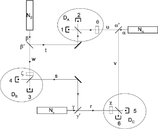
Figure 4: Interferometer with three Fock-state condensate sources and three detectors. The particles from each source can reach two detectors. Each detector has two subdetectors, which will register a $+1$ for the odd-numbered subdetector and $-1$ for the even-numbered. We average the quantity $\mathcal{ABC}$ where $\mathcal{A}=\pm 1$ for Alice’s detector, and $\mathcal{B}=\pm 1$ for Bob’s, and $\mathcal{C}=\pm 1$ for Carole’s.

The initial TFS is:

$$\left|\Phi\right\rangle~{}=\left|N_{\alpha},N_{\beta},N_{\gamma}\right\rangle=\frac{1}{\sqrt{N_{\alpha}!N_{\beta}!N_{\gamma}!}}a_{\alpha}^{\dagger N_{\alpha}}a_{\beta}^{\dagger N_{\beta}}a_{\gamma}^{\dagger N_{\gamma}}\left|0\right\rangle$$ (74)

As in § 1, the output modes (destruction operators) $a_{1}\cdots a_{6}$ can be written in terms of the modes at the sources $a_{\alpha},a_{\beta}$ and $a_{\gamma}$ with three phase shifts of $\zeta,$ $\chi,$ or $\theta$. We find:

$$a_{1} =\frac{1}{2}\left[e^{i\zeta}a_{\alpha}-ia_{\beta}\right],~{}\text{~{}}~{}\text{~{}}~{}\text{~{}}~{}a_{2}=\frac{1}{2}\left[ie^{i\zeta}a_{\alpha}-a_{\beta}\right],$$

$$a_{3} =\frac{1}{2}\left[e^{i\theta}a_{\beta}-ia_{\gamma}\right],~{}\text{~{}}~{}\text{~{}}~{}\text{~{}}~{}a_{4}=\frac{1}{2}\left[ie^{i\theta}a_{\beta}-a_{\gamma}\right],$$

$$a_{5} =\frac{1}{2}\left[-a_{\alpha}+e^{i\chi}a_{\gamma}\right],\text{~{}~{}}~{}\text{~{}}~{}\text{~{}}a_{6}=\frac{1}{2}\left[ia_{\alpha}+ie^{i\chi}a_{\beta}\right].$$ (75)

We write generally $a_{i}=v_{i\alpha}a_{\alpha}+v_{i\beta}a_{\beta}+v_{i\gamma}a_{\gamma}$. We consider only the case where every particle in the source is detected, so the probability that we find $m_{i}$ particles in detector $i=1\cdots 6,$ is:

$$\mathcal{P(}m_{1},\cdots,m_{6})\sim\frac{1}{m_{1}!\cdots m_{6}!}\left|\left\langle 0\right|a_{1}^{m_{1}}\cdots a_{6}^{m_{6}}\left|N_{\alpha},N_{\beta},N_{\gamma}\right\rangle\right|^{2}$$ (76)

(this relation is actually an equality, but we write it only as a proportionality relation since we will change the normalization below). We can develop the matrix element just as we did in § 1.1:

$$\begin{array}[c]{l}\displaystyle\left\langle 0\right|\prod_{i=1}^{6}\left(v_{i\alpha}a_{\alpha}+v_{i\beta}a_{\beta}+v_{i\gamma}a_{\gamma}\right)^{m_{i}}a_{\alpha}^{\dagger N_{\alpha}}a_{\beta}^{\dagger N_{\beta}}a_{\gamma}^{\dagger N_{\gamma}}\left|0\right\rangle=N_{\alpha}!N_{\beta}!N_{\gamma}!~{}\times\\ \lx@intercol\hfil\displaystyle\times\sum_{p_{1=0}}^{m_{1}}...\sum_{p_{6=0}}^{m_{6}}\left[\prod_{i=1}^{6}\left(\frac{m_{i}!}{p_{i\alpha}!p_{i\beta}!p_{i\gamma}!}u_{i\alpha}^{p_{i\alpha}}u_{i\beta}^{p_{i\beta}}u_{i\gamma}^{p_{i\gamma}}\right)~{}\delta_{p_{1\alpha}+\cdots+p_{6\alpha},N_{\alpha}}~{}\delta_{p_{1\beta}+\cdots+p_{6\beta},N_{\beta}}~{}\delta_{p_{1\gamma}+\cdots+p_{6\gamma},N_{\gamma}}\right]\lx@intercol\end{array}$$ (77)

where the sums are over all $p_{i\alpha}$, $p_{i\beta}$ and $p_{i\gamma}$ such that $p_{i\alpha}+p_{i\beta}+p_{i\gamma}=m_{i}$. We now replace the $\delta$-functions by integrals:

$$\delta_{p_{1\alpha}+\cdots+p_{6\alpha},N_{\alpha}}=\int_{-\pi}^{\pi}\frac{d\lambda_{\alpha}}{(2\pi)^{3}}e^{i(p_{1\alpha}+\cdots+p_{6\alpha}-N_{\alpha})\lambda_{\alpha}}$$ (78)

with similar integrals over $\lambda_{\beta}$ and $\lambda_{\gamma}.$ In the sum above then, we have every $v_{i\alpha}^{p_{i\alpha}}$ replaced by $\left(v_{i\alpha}e^{i\lambda_{\alpha}}\right)^{p_{i\alpha}}$ etc. so that we can redo the sums over the $p_{i\alpha},$ etc. to find the probability for the $m_{i}$ arrangement under the condition that all the source particles are detected:

$$\mathcal{P(}m_{1},\cdots,m_{6})\sim\frac{1}{m_{1}!\cdots m_{6}!}\int d\tau^{\prime}\int d\tau e^{-i[N_{\alpha}(\lambda_{\alpha}-\lambda_{\alpha}^{\prime})+N_{\beta}(\lambda_{\beta}-\lambda_{\beta}^{\prime})+N_{\gamma}(\lambda_{\gamma}-\lambda_{\gamma}^{\prime})]}\prod_{i=1}^{6}\left(\Omega_{i}^{\prime\ast}\Omega_{i}\right)^{m_{i}}$$ (79)

where $\Omega_{i}$ $=v_{i\alpha}e^{i\lambda_{\alpha}}+v_{i\beta}e^{i\lambda_{\beta}}+v_{i\gamma}e^{i\lambda_{\gamma}}$ and $\Omega_{i}^{\prime}$ has the same expression with primed $\lambda$’s; $d\tau$ represents the integrals over $\lambda_{\alpha},$ $\lambda_{\beta},$ and $\lambda_{\gamma},$ and $d\tau^{\prime}$ over the $\lambda_{\alpha}^{\prime},$ $\lambda_{\beta}^{\prime},$ and $\lambda_{\gamma}^{\prime}.$

In a ideal experiment with 100% detection efficiency, the numbers of particles detected in each region are EPR variables, since the value of two of these variables determines the value of the third with certainty; these perfect correlations are independent of the settings (phase shifts of $\zeta,$ $\chi,$ or $\theta$), so that choosing the number of detections in each region defines a class of events that is independent of the settings. Here, assuming that each source emits $N/3$ particles (otherwise, we find zero average values, see below):

$$N_{\alpha}=N_{\beta}=N_{\gamma}=N/3$$

we will also assume that each detector registers exactly $N/3$ particles. We can put in this restriction, when we sum on $m_{1}\cdots m_{6}$ to get averages, by including three $\delta$-functions of the form:

$$\delta_{m_{1}+m_{2},N/3}=\int_{-\pi}^{\pi}\frac{d\rho_{A}}{2\pi}~{}e^{i\rho_{A}(m_{1}+m_{2}-N/3)}$$ (80)

with similar ones specifying $m_{3}+m_{4}=N/3$ and $m_{5}+m_{6}=N/3$. The $m_{i}$ sums are then done independently of one another giving a normalization sum of:

$$\mathcal{N} =\int d\tau_{\rho}\int d\tau^{\prime}\int d\tau e^{-i[N_{\alpha}(\lambda_{\alpha}-\lambda_{\alpha}^{\prime})+N_{\beta}(\lambda_{\beta}-\lambda_{\beta}^{\prime})+N_{\gamma}(\lambda_{\gamma}-\lambda_{\gamma}^{\prime})]}$$

$$\times e^{-iN/3[\rho_{A}+\rho_{B}+\rho_{C}]}\exp\left[\sum_{i=1}^{6}\left(\Omega_{i}^{\prime\ast}\Omega_{i}e^{i\rho_{i}}\right)\right]$$ (81)

where $\rho_{1}=\rho_{2}=\rho_{A},$ $\rho_{3}=\rho_{4}=\rho_{B},$ and $\rho_{5}=\rho_{6}=\rho_{C}$ and $\int d\tau_{\rho}$ represents the new three-fold integration. The sum in the exponential is easily done:

$$\sum_{i=1}^{6}\left(\Omega_{i}^{\prime\ast}\Omega_{i}e^{i\rho_{i}}\right) =\frac{1}{2}\left[e^{-i(\lambda_{\alpha}-\lambda_{\alpha}^{\prime})}\left(e^{i\rho_{A}}+e^{i\rho_{C}}\right)\right.$$

$$\left.+e^{-i(\lambda_{\beta}-\lambda_{\beta}^{\prime})}\left(e^{i\rho_{B}}+e^{i\rho A}\right)+e^{i(\lambda_{\gamma}-\lambda_{\gamma}^{\prime})]}\left(e^{i\rho_{C}}+e^{i\rho_{B}}\right)\right]$$ (82)

We expand the exponential of this quantity in series in $e^{-i(\lambda_{\alpha}-\lambda_{\alpha}^{\prime})},$ $e^{-i(\lambda_{\beta}-\lambda_{\beta}^{\prime})},$ and $e^{i(\lambda_{\gamma}-\lambda_{\gamma}^{\prime})}$ and do the integrals. When each source emits exactly $N/3$ particles, we obtain:

$$\mathcal{N}=\frac{1}{2^{N}}\sum_{l=0}^{\infty}\left(\frac{1}{l!(\frac{N}{3}-l)!}\right)^{3}$$ (83)

Similarly we average the quantities $\mathcal{A},$ $\mathcal{B},$ and $\mathcal{C}$ each $\pm 1$ measured by Alice, Bob, and Carole according to:

$$\left\langle\mathcal{ABC}\right\rangle=\sum_{m_{1}\cdots m_{6}}{}^{\prime}(-1)^{m_{2}+m_{4}+m_{6}}\mathcal{P(}m_{1},\cdots,m_{6})$$ (84)

where the prime on the sum means we again restrict the sums to the case of $N/3$ particles reaching each detector. With this requirement the average vanishes unless each source emits exactly $N/3$ particles, which is why above we considered just that case. We have then:

$$\left\langle\mathcal{ABC}\right\rangle=\frac{\sum_{q}\left(\frac{N/3!}{(N/3-q)!q!}~{}\right)^{3}e^{i(\zeta+\theta+\chi)(N/3-2q)}}{\sum_{q}\left(\frac{N/3!}{(N/3-q)!q!}~{}\right)^{3}}$$ (85)

Note that if $\zeta+\theta+\chi=0$ we find $\left\langle\mathcal{ABC}\right\rangle=1$: perfect correlations exist between the results since their product is fixed. Thus, if we know the parity of the results of two of the experimenters, we immediately know that of the third, even if that person is very far away. Thus an EPR argument applies to these variables.

For the case $N=3,$ we find $\left\langle\mathcal{ABC}\right\rangle=\cos(\zeta+\theta+\chi),$ which is the same form of the original GHZ case found from a three-body NOON state. This result agrees with the interferometer result of Ref. [38] as expected. Local realism predicts that, for each realization of the experiment, the product of the results is given by a product $A(\zeta)B(\theta)C(\chi)$. To get agreement with quantum mechanics in situations of perfect correlations we must have:

$$A(\pi/2)~{}B(\pi/2)~{}C(0) =-1$$

$$A(\pi/2)~{}B(0)~{}C(\pi/2) =-1$$

$$A(0)~{}B(\pi/2)~{}C(\pi/2) =-1$$ (86)

But then we obtain by product $A(0)B(0)C(0)=-1,$ while quantum mechanics gives $+1$, in complete contradiction. In our case we get new contradictions for larger $N$; consider for instance $N=9,$ in which case:

$$\left\langle\mathcal{ABC}\right\rangle=\frac{1}{28}\left[27\cos(\zeta+\theta+\chi)+\cos 3(\zeta+\theta+\chi)\right]$$ (87)

The above argument goes through exactly in the same way. More generally, any time $N/3$ is odd we get a similar result for arbitrary $N.$

Thus the TFS provides new GHZ-type contradictions for $N$ particles without having to prepare NOON states.

3.3 Hardy impossibilities

Hardy impossibilities are treated by use of the interferometer shown in Fig. 5, based on the one discussed in Ref. [46] for $N=2$.

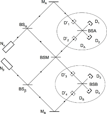
Figure 5: An interferometer with particle sources $\alpha$ and $\beta$, with beam splitters designated by BS and mirrors by M. In both detection regions, the detectors at D_i may be replaced by the D${}_{i}^{\prime}$, placed before the beam splitters.

The heart of the system is the beam splitter at the center; due to Bose interference it has the property that, if an equal number of particles approaches each side, then an even number must emerge from each side. The detection beam splitters BSA and BSB are each set to have a transmission probability of 1/3, and the path differences are such that, by destructive interference, no particle reaches $D_{2}$ if only source $N_{\alpha}$ is used; similarly, no particle reaches $D_{3}$ if $N_{\beta}$ alone is used. Alice can use either the detectors $D_{1,2}$ after her beam splitter, or $D_{1,2}^{\prime}$ before; Bob can choose either D_3,4, or D${}_{3,4}^{\prime}$. This gives $4$ arrangements of experiments: $DD$, $DD^{\prime}$, $D^{\prime}D$, or $D^{\prime}D^{\prime}$, with probability amplitudes $C_{XY}(m_{1},m_{2};m_{3},m_{4})$, where $XY$ is any of these $4$ arrangements and the $m$ values are the numbers of particles detected at each counter.

We find the destruction operators for the detector modes as we have done in previous sections. For the primed detectors we find:

$$\begin{array}[c]{l}a_{D_{1}^{\prime}}=\frac{i}{\sqrt{2}}a_{\alpha},~{}\text{~{}}~{}\text{~{}}~{}\text{~{}}~{}\text{~{}}~{}\text{~{}}~{}\text{~{}}~{}\text{~{}}a_{D_{2}^{\prime}}=\frac{1}{2}\left(-a_{\alpha}+ia_{\beta}\right)\\ a_{D_{3}^{\prime}}=\frac{1}{2}\left(ia_{\alpha}-a_{\beta}\right),~{}\text{~{}}~{}a_{D_{4}^{\prime}}=\frac{i}{\sqrt{2}}a_{\beta}\end{array}$$ (88)

and for the unprimed detectors:

$$\begin{array}[c]{l}a_{D_{1}}=-\frac{\sqrt{3}}{2}a_{\alpha}+\frac{i}{2\sqrt{3}}a_{\beta},~{}\text{~{}}~{}\text{~{}}~{}\text{~{}}~{}a_{D_{2}}=-\frac{1}{\sqrt{6}}a_{\beta}\\ a_{D_{3}}=-\frac{1}{\sqrt{6}}a_{\alpha},~{}\text{~{}}~{}\text{~{}}~{}\text{~{}}~{}\text{~{}}~{}\text{~{}}~{}\text{~{}}~{}\text{~{}}~{}\text{~{}}~{}\text{~{}}~{}\text{~{}}~{}a_{D_{4}}=\frac{i}{2\sqrt{3}}a_{\alpha}-\frac{\sqrt{3}}{2}a_{\beta}\end{array}$$ (89)

In general we write these results as:

$$a_{i}=v_{i\alpha}a_{\alpha}+v_{i\beta}a_{\beta}$$ (90)

Note that, because of the $1/3$ transmission probability at BSA and BSB, Bose interference causes $a_{\alpha}$ and $a_{\beta}$ to drop out of the second and third of Eqs (89), respectively.

The amplitude is given by:

$$C_{\mathrm{XY}}(m_{1},m_{2};m_{3},m_{4})\sim\left\langle 0\right|\prod_{i=1}^{6}\left(v_{i\alpha}a_{\alpha}+v_{i\beta}a_{\beta}\right)^{m_{i}}a_{\alpha}^{\dagger N_{\alpha}}a_{\beta}^{\dagger N_{\beta}}\left|0\right\rangle$$ (91)

As we have done in previous sections, we expand the binomials, evaluate the operator matrix element, replace the resulting $\delta$-functions by integrals and resum the series to find:

$$C_{\mathrm{XY}}(m_{1},m_{2};m_{3},m_{4})\sim\int_{-\pi}^{\pi}\frac{d\lambda_{\alpha}}{2\pi}\int_{-\pi}^{\pi}\frac{d\lambda_{\beta}}{2\pi}e^{{}^{-iN_{\alpha}\lambda_{\alpha}}}e^{{}^{-iN_{\beta}\lambda_{\beta}}}\prod_{i=1}^{4}\left(v_{i\alpha}e^{i\lambda_{\alpha}}+v_{i\beta}e^{i\lambda_{\beta}}\right)^{m_{i}}$$ (92)

In all the following we assume that each source emits $N/2$ particles, where $N/2$ is odd, and that detector A and detector B each receive exactly $N/2$ particles; this is possible since, as above, the number of particles detected in each region can define a sample of realizations that is independent of the settings (we have to make this assumption since it turns out that the argument works only in this case). First consider both Alice and Bob using primed detectors. The amplitude for receiving $N/2$ particles in each of D${}_{2}^{\prime}$ and D${}_{3}^{\prime}$ is:

$$C_{\mathrm{D}^{\prime}\mathrm{D}^{\prime}}(0,\frac{N}{2};0,\frac{N}{2}) \sim\int_{-\pi}^{\pi}\frac{d\lambda_{\alpha}}{2\pi}\int_{-\pi}^{\pi}\frac{d\lambda_{\beta}}{2\pi}e^{{}^{-i\frac{N}{2}(\lambda_{\alpha}+\lambda_{\beta})}}\left(-e^{i\lambda_{\alpha}}+ie^{i\lambda_{\beta}}\right)^{N/2}\left(ie^{i\lambda_{\alpha}}-e^{i\lambda_{\beta}}\right)^{N/2}$$

$$\sim\int_{-\pi}^{\pi}\frac{d\lambda_{\alpha}}{2\pi}\int_{-\pi}^{\pi}\frac{d\lambda_{\beta}}{2\pi}e^{{}^{-i\frac{N}{2}(\lambda_{\alpha}+\lambda_{\beta})}}\left(e^{i2\lambda_{\alpha}}+e^{i2\lambda_{\beta}}\right)^{N/2}=0$$ (93)

This quantity must vanish because $N/2$ is odd. This situation is an example of the beam splitter rule mentioned above. The result is that D${}_{2}^{\prime}$ and D${}_{3}^{\prime}$ cannot collect all the particles if $N/2$ are detected on each side.

Consider next the case where one experimenter uses a primed set of detectors and the other the unprimed:

$$C_{\mathrm{DD}^{\prime}}(0,\frac{N}{2};m_{3}^{\prime},m_{4}^{\prime}) \sim\int_{-\pi}^{\pi}\frac{d\lambda_{\alpha}}{2\pi}\int_{-\pi}^{\pi}\frac{d\lambda_{\beta}}{2\pi}e^{{}^{-i\frac{N}{2}(\lambda_{\alpha}+\lambda_{\beta})}}\left(e^{i\lambda_{\beta}}\right)^{N/2}\left(ie^{i\lambda_{\alpha}}-e^{i\lambda_{\beta}}\right)^{m_{3}^{\prime}}\left(e^{i\lambda_{\beta}}\right)^{m_{4}^{\prime}}$$

$$\sim\delta_{m_{4}^{\prime},0}$$ (94)

The factor $\left(e^{i\lambda_{\beta}}\right)^{N/2}$ combines with the first exponential so that $m_{4}^{\prime}$ must vanish. This quantity vanishes because of the destructive interference effects at BSA and BSB caused by the 1/3 transmission probability of the beam splitters; but $C_{\mathrm{DD}^{\prime}}(0,\frac{N}{2};\frac{N}{2},0)\neq 0$. Thus, if Alice observes $N/2$ particles at D₂, when Bob uses the primed detectors he observes with certainty $N/2$ particles at D${}_{3}^{\prime}$; similarly, if Bob has seen $N/2$ particles in D₃, in the D^′D configuration Alice must see $N/2$ in D${}_{2}^{\prime}$ .

We now consider events where both experimenters do unprimed experiments and each of them finds $N/2$ particles in D₂ and D₃; the corresponding probability is:

$$C_{\mathrm{DD}}(0,\frac{N}{2};\frac{N}{2},0)\sim\int_{-\pi}^{\pi}\frac{d\lambda_{\alpha}}{2\pi}\int_{-\pi}^{\pi}\frac{d\lambda_{\beta}}{2\pi}e^{{}^{-i\frac{N}{2}(\lambda_{\alpha}+\lambda_{\beta})}}\left(e^{i\lambda_{\beta}}\right)^{N/2}\left(e^{i\lambda_{\alpha}}\right)^{N/2}\neq 0,$$ (95)

(for $N=6$, the normalized value is $1/216$), which means that events exist where $N/2$ particles are detected at both detectors D₂ and D₃. However, in any of these events, if Bob had at the last instant changed to the primed detectors, he would surely have obtained $N/2$ particles in D${}_{3}^{\prime}$, because of the certainty mentioned above (while Alice still has $N/2$ particles in D₂). Similarly, if it is Alice who chooses primed detectors at the last moment, she always obtains $N/2$ particles in D${}_{2}^{\prime}$ (while Bob continues to have $N/2$ particles in D₃). Now, had both changed their minds after the emission and chosen the primed arrangement, local realism implies that they would have found $N/2$ particles each in D${}_{2}^{\prime}$ and D${}_{3}^{\prime}$: such events must exist. But the corresponding quantum probability is zero, in complete contradiction. The result is the Hardy impossibility of Ref. [46] generalized to $N$ particles.

4 Conclusion

Fock-state condensates appear as remarkably versatile, able to create violations that usually require elaborate entangled wave functions, and produce new $N$-body violations. Compared to GHZ states or other elaborate quantum states, they have the advantage of being accessible through the phenomenon of Bose-Einstein condensation, with no limitation in principle concerning the number of particles involved. By contrast, the production of GHZ states requires elaborate measurement procedures, so that it seems difficult to produce them with more than a few particles (to our knowledge, the present world record is 5, see [54]); moreover, they are much more sensitive to decoherence, which destroys their quantum coherence properties [33].

From an experimental point of view, the major requirement is that all particles present in the initial double Fock state should be detected, which will of course put a practical limit on the number of particles involved. Using Bose condensed gases of metastable He atoms seems to be an attractive possibility, since the detection of individual atoms is possible with micro-channel plates [18, 19]. With alkali atoms, one could also measure the position of the particles at the outputs of interferometers by laser fluorescence, obtaining a non-destructive quantum measurement of $m_{1}$, ..$m_{4}$. The realization of interferometers seems also possible, since interferometry with Bose-Einstein condensates has already been performed [55] with the help of Bragg scattering optical beam splitters [56, 57]. Another possibility may be to use cavity quantum electrodynamics and quantum non-demolition photon counting methods [58] to prepare multiple Fock states. Experiments therefore do not seem to be out of reach.

Laboratoire Kastler Brossel is “UMR 8552 du CNRS, de l’ENS, et de l’Université Pierre et Marie Curie”.

APPENDIX I

In this appendix, we give some formulas that are useful for the calculations of this article, in particular to check the normalization of (15) and (24).

(i) Wallis integral. We consider the integral:

$$K=\int_{-\pi}^{+\pi}\frac{d\lambda}{2\pi}~{}\left[\cos\lambda\right]^{N}$$ (96)

which, if the limits are changed to $0$ and $\pi/2$, becomes a Wallis integral (divided by $2\pi$ if one takes the usual definition of these integrals). Expanding the integrand provides:

$$2^{-N}\left[e^{i\lambda}+e^{-i\lambda}\right]^{N}=2^{-N}\sum_{q=0}^{N}\frac{N!}{q!(N-q)!}~{}e^{i\left(N-2q\right)\lambda}$$ (97)

The only exponentials that survive the $\lambda$ integration are those with vanishing exponent ($N-2q=0$). Therefore:

$$\begin{array}[c]{l}\text{if }N\text{ is odd, }K=0\\ \text{if }N\text{ is even, }K=2^{-N}\frac{N!}{\left[(N/2)!\right]^{2}}\end{array}$$ (98)

(ii) Normalization integral. We define:

$$J=\int_{-\pi}^{+\pi}\frac{d\Lambda}{2\pi}\cos\left[\left(N_{\alpha}-N_{\beta}\right)\Lambda\right]\left[\cos\Lambda\right]^{M}=\operatorname{Re}\left\{\int_{-\pi}^{+\pi}\frac{d\Lambda}{2\pi}e^{i\left(N_{\alpha}-N_{\beta}\right)\Lambda}\left[\cos\Lambda\right]^{M}\right\}$$ (99)

and expand:

$$\left[\cos\Lambda\right]^{M}=\left[\frac{e^{i\Lambda}+e^{-i\Lambda}}{2}\right]^{M}=2^{-M}\sum_{q=0}^{M}\frac{M!}{q!(M-q)!}~{}e^{i\left(M-2q\right)\lambda}$$ (100)

Only a term with $M-2q=N_{\alpha}-N_{\beta}$ can survive the integration, so that:

$$q=\frac{N_{\beta}-N_{\alpha}-M}{2}$$ (101)

Therefore, $J$ is non-zero only if:

$$M\text{ has the same parity as }N_{\alpha}-N_{\beta}\text{ \ ; \ }-M\leq N_{\alpha}-N_{\beta}\leq+M$$ (102)

and then:

$$J=2^{-M}\frac{M!}{\left(\frac{M+N_{\alpha}-N_{\beta}}{2}\right)!\left(\frac{M-N_{\alpha}+N_{\beta}}{2}\right)!}$$ (103)

(iii) Normalization of (15). We now consider the probabilities $\mathcal{P(}m_{1},m_{2},m_{3},m_{4})$ given by (15) and calculate their sum over $m_{1},m_{2},m_{3},m_{4}$, when these variables have a constant sum $N$. We do these sums in three steps: a summation over $m_{1}$ and $m_{2}$ (with constant sum $m_{A}$), a summation over $m_{3}$ and $m_{4}$ (with constant sum $m_{A}$), and a summation over $m_{A}$ and $m_{B}$ (with constant sum $M$). The first two sums reconstruct powers of a binomial, the $\lambda$ integral disappears, and we obtain:

$$N_{\alpha}!N_{\beta}!~{}2^{-N}\int_{-\pi}^{+\pi}\frac{d\Lambda}{2\pi}\cos\left[\left(N_{\alpha}-N_{\beta}\right)\Lambda\right]\times\frac{1}{m_{A}!m_{B}!}\left[2\cos\Lambda\right]^{N}$$ (104)

which, with (103) for $M=N=N_{\alpha}+N_{\beta}$, gives:

$$2^{-N}\text{~{}}\times\frac{M!}{m_{A}!m_{B}!}$$ (105)

Then the summation over $m_{A}$ and $m_{B}$ gives:

$$2^{-N}\left(1+1\right)^{N}=1$$ (106)

as expected.

(iv) Normalization of (24). We now consider the probabilities $\mathcal{P(}m_{1},m_{2},m_{3},m_{4})$ given by (24) and calculate their sum over any $m_{1},m_{2},m_{3},m_{4}$. We do this by the same three summation as above (with $m_{A}+m_{B}=M$, instead of $N$), plus a summation over $M$ ranging from $0$ to $N$. The first two summations give:

$$\frac{N_{\alpha}!N_{\beta}!}{m_{A}!m_{B}!}\frac{2^{N-2M}}{\left(N-M\right)!}T^{M}R^{N-M}\int_{-\pi}^{+\pi}\frac{d\Lambda}{2\pi}\cos\left[\left(N_{\alpha}-N_{\beta}\right)\Lambda\right]\left[\cos\Lambda\right]^{N-M}\left[2\cos\Lambda\right]^{M}$$ (107)

or, when (103) is inserted:

$$\frac{N!}{m_{A}!m_{B}!}\frac{2^{-M}}{\left(N-M\right)!}T^{M}R^{N-M}$$ (108)

The summation over $m_{A}$ and $m_{B}$ with constant sum $M$ then gives:

$$\frac{N!}{M!\left(N-M\right)!}T^{M}R^{N-M}$$ (109)

which provides the probability of detecting $M$ particles, independently of which of the 4 detectors is activated. This probability is maximal when:

$$\frac{N-M}{M}\frac{T}{R}\sim 1~{}\ \ \ \ \ \ \ \text{\ or \ \ \ \ \ \ \ }\frac{M}{N}\sim T$$ (110)

The larger the transmission coefficient $T$, the larger the most likely value of $M$, as one could expect physically. Finally, a summation of (109) over $M$ between $0$ and $N$ gives:

$$\left(R+T\right)^{N}=1$$ (111)

and the total probability is $1$, as expected.

APPENDIX II

In this appendix, we investigate how Eq. (15) is changed when the initial state $\left|\Phi_{0}\right\rangle$ is different from the double Fock state considered in (1).

(a) Coherent states

We first assume that each of the modes $\alpha$, $\beta$ is in a coherent state with phases $\phi_{\alpha}$, $\phi_{\beta}$ and the same amplitude $E$:

$$\left|\Phi_{0}\right\rangle=\left|\phi_{\alpha}\right\rangle\otimes\left|\phi_{\beta}\right\rangle$$ (112)

with the usual expression of the coherent states:

$$\left|\phi_{\alpha,\beta}\right\rangle\sim\sum_{r=0}^{\infty}\frac{\left[E~{}e^{i\phi_{\alpha,\beta}}\right]^{r}}{\sqrt{r!}}\left|N_{\alpha,\beta}=r\right\rangle$$ (113)

The calculation of § 1.1 is then simplified since this state is a common eigenvector of both annihilation operators $a_{\alpha}$ and $a_{\beta}$. There is no need to introduce conservation rules, and neither $\lambda$ nor $\Lambda$ enter the expressions. Eq. (15) becomes:

$$\begin{array}[c]{l}\mathcal{P(}m_{1},m_{2},m_{3},m_{4})\sim\left[1+\cos\left(\zeta+\phi_{\alpha}-\phi_{\beta}\right)\right]^{m_{1}}\left[1-\cos\left(\zeta+\phi_{\alpha}-\phi_{\beta}\right)\right]^{m_{2}}\\ \lx@intercol\hfil\times\left[1+\cos\left(\theta+\phi_{\beta}-\phi_{\alpha}\right)\right]^{m_{3}}\left[1-\cos\left(-\theta+\phi_{\beta}-\phi_{\alpha}\right)\right]^{m_{4}}\lx@intercol\end{array}$$ (114)

Here, no $\lambda$ distribution occurs, in contrast with (15): the relative phase of the two states is perfectly defined and takes the exact value $\phi_{\alpha}-\phi_{\beta}$. Now, we can also assume that the initial phases of the two coherent states completely random. Then, an average over all possible values of $\phi_{\alpha}$and $\phi_{\beta}$ leads to:

$$\begin{array}[c]{l}\mathcal{P(}m_{1},m_{2},m_{3},m_{4})\sim\int\frac{d\phi}{2\pi}~{}\left[1+\cos\left(\zeta+\phi\right)\right]^{m_{1}}\left[1-\cos\left(\zeta+\phi\right)\right]^{m_{2}}\\ \lx@intercol\hfil\left[1+\cos\left(-\theta+\phi\right)\right]^{m_{3}}\left[1-\cos\left(-\theta+\phi\right)\right]^{m_{4}}\lx@intercol\end{array}$$ (115)

We now obtain an expression that is similar to Eq. (15), but with a difference: the terms of the product in the integral are always positive, as if the quantum angle $\Lambda$ had been set equal to zero; no violation of Bell inequalities is therefore possible. This was expected: with coherent states, the phase pre-exists the measurement and is not created under the effect of quantum measurement, as was the case with Fock states; an unknown classical variable does not lead to violations local realism. Moreover, the requirement of measuring all particles does not apply in this case, since the initial state does not have an upper bound for the populations.

(b) Phase state

We now assume choose a state that has a fixed number of particles, but a well defined phase $\phi_{0}$ between the two modes:

$$\left|\Phi_{0},N\right\rangle=\frac{1}{\sqrt{N!}}\left[e^{i\phi_{0}}a_{\alpha}^{\dagger}+a_{\beta}^{\dagger}\right]^{N}\left|0\right\rangle=\sqrt{N!}\sum_{q=0}^{N}~{}\frac{e^{iq\phi_{0}}}{q!\left(N-q\right)!}~{}\left(a_{\alpha}^{\dagger}\right)^{q}\left(a_{\beta}^{\dagger}\right)^{N-q}\left|0\right\rangle$$ (116)

with $N$ even. We assume that all particles are measured: $\sum_{i}m_{i}=N$. The probability amplitude we wish to calculate is:

$$C_{m_{1}\cdots m_{4}}=\frac{1}{\sqrt{\prod_{j}m_{j}!}}\left\langle 0\right|\prod_{j=1}^{4}a_{j}^{m_{j}}\left|\Phi_{0},N\right\rangle$$ (117)

where the $a_{i}$ are defined in (3) and written more generically in (4). We will use two different methods to do the calculation, first a method based on the specific properties of phase states, and then a more generic method extending the results of § 1.1.

(i) The phase state $\left|\Phi_{0},N\right\rangle$ is by definition a state where all bosons are created in one single state $\left[e^{i\phi_{0}}\left|\alpha\right\rangle+\left|\beta\right\rangle\right]/\sqrt{2}$, none in the orthogonal state $\left[-e^{i\phi_{0}}\left|\alpha\right\rangle+\left|\beta\right\rangle\right]/\sqrt{2}$. Therefore the action of the two annihilation operators:

$$\begin{array}[c]{l}a_{\phi_{0}}=\frac{e^{-i\phi_{0}}a_{\alpha}+a_{\beta}}{\sqrt{2}}\\ a_{\phi_{0+\pi}}=\frac{-e^{-i\phi_{0}}a_{\alpha}+a_{\beta}}{\sqrt{2}}\end{array}$$ (118)

is straightforward: the former transforms $\left|\Phi_{0},N\right\rangle$ into $\left|\Phi_{0},N-1\right\rangle$, the latter gives zero. Now, we can use (4) and (118) to expand each $a_{i}$ as:

$$a_{j}=v_{j\alpha}e^{i\phi_{0}}\frac{a_{\phi_{0}}-a_{\phi_{0+\pi}}}{\sqrt{2}}+v_{j\beta}\frac{a_{\phi_{0}}+a_{\phi_{0+\pi}}}{\sqrt{2}}$$ (119)

where the action of $a_{\phi_{0+\pi}}$ gives zero. We conclude that:

$$a_{j}\left|\Phi_{0},N\right\rangle=\sqrt{\frac{N}{2}}(e^{i\phi_{0}}v_{j\alpha}+v_{j\beta})\left|\Phi_{0},N-1\right\rangle$$ (120)

in which case:

$$C_{m_{1}\cdots m_{4}}=\sqrt{\frac{N!}{2^{N}\prod_{j}m_{j}!}}\prod_{j=1}^{4}(e^{i\phi_{0}}v_{j\alpha}+v_{j\beta})^{m_{j}}$$ (121)

The probability is then:

$$\begin{array}[c]{l}\displaystyle\mathcal{P}(m_{1},m_{2},m_{3},m_{4})=\frac{N!}{\prod_{j}2^{N}m_{j}!}\prod_{j=1}^{4}\left[(e^{-i\phi_{0}}v_{j\alpha}^{\ast}+v_{j\beta}^{\ast})(e^{i\phi_{0}}v_{j\alpha}+v_{j\beta})\right]^{m_{j}}\\ \lx@intercol\hfil\displaystyle=\frac{N!}{4^{N}~{}m_{1}!...m_{4}!}\left[(1+\cos(\zeta+\phi_{0})\right]^{m_{1}}\left[(1-\cos(\zeta+\phi_{0})\right]^{m_{2}}\hfil\lx@intercol\\ \lx@intercol\hfil\displaystyle\times\left[(1+\cos(\theta-\phi_{0})\right]^{m_{3}}\left[(1-\cos(\theta-\phi_{0})\right]^{m_{4}}\lx@intercol\end{array}$$ (122)

As in case (a), we have a state for which the quantum angle vanishes so that no violation of the BCHSH inequalities can take place.

(ii) We can also do the calculation by a method that is similar to that of § 1.1. From (116) and (117), we obtain:

$$C_{m_{1}\cdots m_{4}}=\frac{\sqrt{N!}}{\sqrt{\prod_{j}m_{j}!}}\sum_{q=0}^{N}~{}\frac{e^{iq\phi_{0}}}{q!\left(N-q\right)!}~{}\prod_{j=1}^{4}~{}\left\langle 0\right|a_{j}^{m_{j}}\left(a_{\alpha}^{\dagger}\right)^{q}\left(a_{\beta}^{\dagger}\right)^{N-q}\left|0\right\rangle$$

The calculation is the same as in § 1.1, with $N_{\alpha}$ replaced by $q$ and $N_{\beta}$ by $N-q$; the prefactors of (1) and (116) combine to introduce a factor $\sqrt{N!/q!\left(N-q\right)!}$, and the equivalent of (10) is now:

$$\sqrt{N!}\sum_{q=0}^{N}e^{iq\phi_{0}}\int_{-\pi}^{\pi}\frac{d\mu}{2\pi}e^{{}^{i\left(N-2q\right)\mu}}\prod_{j=1}^{4}\left(v_{j\alpha}e^{i\mu}+v_{j\beta}e^{-i\mu}\right)^{m_{j}}$$ (123)

In the probability, a sum over $q$ and $q^{\prime}$ appears, including term $q\neq q^{\prime}$ corresponding to non-diagonal probability terms between two different states $\left\langle N_{\alpha}=q^{\prime}~{};N_{\beta}=N-q^{\prime}\right|$ and $\left|N_{\alpha}=q~{};N_{\beta}=N-q\right\rangle$. One finally obtains:

$$\begin{array}[c]{l}\displaystyle\mathcal{P(}m_{1},m_{2},m_{3},m_{4})=\frac{N!}{m_{1}!m_{2}!m_{3}!m_{4}!}2^{-N}\int_{-\pi}^{\pi}\frac{d\lambda}{2\pi}\int_{-\pi}^{\pi}\frac{d\Lambda}{2\pi}~{}G\left(\lambda,\Lambda\right)~{}\left[\cos\Lambda+\cos\left(\zeta+\lambda\right)\right]^{m_{1}}\\ \displaystyle\times\left[\cos\Lambda-\cos\left(\zeta+\lambda\right)\right]^{m_{2}}\left[\cos\Lambda+\cos\left(\theta-\lambda\right)\right]^{m_{3}}\left[\cos\Lambda-\cos\left(\theta-\lambda\right)\right]^{m_{4}}\end{array}$$ (124)

with:

$$G\left(\lambda,\Lambda\right)=\sum_{q,q^{\prime}=0}^{N}e^{i\left(q-q^{\prime}\right)\left(\phi_{0}-\lambda\right)}~{}e^{i\left(N-q-q^{\prime}\right)\Lambda}$$ (125)

The result is therefore similar to (15), except for the presence of the function $G\left(\lambda,\Lambda\right)$, which introduces a distribution of the phase $\lambda$ and of the quantum angle $\Lambda$.

Equations (124) and (125) are equivalent to (122), although they do not contain the same distribution $G\left(\lambda,\Lambda\right)$. Equation (122) corresponds to an infinitely narrow distribution, since it can be obtained by replacing in (124) $G\left(\lambda,\Lambda\right)$ by the product $\delta(\lambda-\phi_{0})$ $\delta(\Lambda)$; by contrast, (125) defines a distribution with finite width. This illustrates the fact that, in (124), different distributions $G\left(\lambda,\Lambda\right)$ may lead to the same set of probabilities.

(c) General state

Consider finally the more general state $\left|\Phi_{0}\right\rangle$ combining two modes with a fixed total number of particles can be written as:

$$\left|\Phi_{0}\right\rangle=\sum_{q=0}^{N}x_{q}~{}\left|N_{\alpha}=q~{};~{}N_{\beta}=N-q\right\rangle$$ (126)

where the complex coefficients $x_{q}$ are arbitrary. The calculation is similar to that of §(ii) above, but now one obtains (124) with a different expression of $G(\lambda,\Lambda)$:

$$G(\lambda,\Lambda)=\sum_{q,q^{\prime}}x_{q}x_{q^{\prime}}^{\ast}~{}e^{i(N-q-q^{\prime})}e^{-i\lambda(q-q^{\prime})}\sqrt{q^{\prime}!(N-q^{\prime})!q!(N-q)!}$$ (127)

Depending on the choice of the coefficients $x_{q}$, one can build states in which the initial phase is well determined, as in § (ii), or completely indetermined as for Fock states; a similar conclusion holds for the quantum angle $\Lambda$.

References

• [1] A. Einstein, B. Podolsky and N. Rosen, “Can quantum mechanical description of physical reality be considered complete?”, Phys. Rev. 47, 777-780 (1935).
• [2] N. Bohr, “Can quantum mechanical description of physical reality be considered complete?”, Phys. Rev. 48, 696-702 (1935)
• [3] J.S. Bell, “On the Einstein-Podolsky-Rosen paradox”, Physics 1, 195-200 (1964); reprinted in [4].
• [4] J.S. Bell, “Speakable and unspeakable in quantum mechanics”, Cambridge University Press (1987).
• [5] S.J. Freedman and J.F. Clauser, “Experimental test of local hidden variable theories”, Phys. Rev. Lett. 28, 938-941 (1972); S.J. Freedman, thesis, University of California, Berkeley; J.F. Clauser, “Experimental investigations of a polarization correlation anomaly”, Phys. Rev. Lett. 36, 1223 (1976).
• [6] E.S. Fry and R.C. Thompson, “Experimental test of local hidden variable theories”, Phys. Rev. Lett. 37, 465-468 (1976).
• [7] A. Aspect, P. Grangier et G. Roger, “Experimental tests of realistic local theories via Bell’s theorem”, Phys. Rev. Lett. 47, 460-463 (1981); “Experimental realization of Einstein-Podolsky-Bohm gedankenexperiment : a new violation of Bell’s inequalities”, 49, 91-94 (1982).
• [8] P.M. Pearle, “Hidden-variable example based on data rejection”, Phys. Rev. D 2, 1418 (1970).
• [9] J. F. Clauser and M.A. Horne, “Experimental consequences of objective local theories”, Phys. Rev. D 10, 526 (1974).
• [10] J.F. Clauser and A. Shimony, “Bell’s theorem: experimental tests and implications”, Rep. on Progress in Phys. 41, 1883-1926 (1978).
• [11] F. Laloë, “Bose-Einstein condensates and quantum non-locality”, page 35 in “Beyond the quantum”, T.M. Nieuwenhuizen, V. Spicka, B. Mehmadi and A. Khrennikov editors, World Scientific (2007); cond-mat/0611043.
• [12] N.D. Mermin, “Extreme quantum entanglement in a superposition of macroscopically distinct states”, Phys. Rev. Lett. 65, 1838 (1990).
• [13] D.M. Greenberger, M.A. Horne and A. Zeilinger, in Bell theorem, quantum theory, and conceptions of the universe, ed. M. Kafatos, (Kluwer, 1989) page 74.
• [14] Greenberger, M.A. Horne, A. Shimony and A. Zeilinger, Am. J. Phys. 58, 1131 (1990).
• [15] P. Drummond, “Violations of Bell’s inequality in cooperative states”, Phys. Rev. Lett. 50, 1407 (1983).
• [16] F. Laloë and W.J. Mullin, “Nonlocal quantum effects with Bose-Einstein condensates”, Phys. Rev. Lett. 99, 150401 (2007).
• [17] F. Laloë and W.J. Mullin, “EPR argument and Bell inequalities for Bose-Einstein spin condensates”, Phys. Rev. A 77, 022108 (2008).
• [18] B. Saubamea, T.W. Hijmans, S. Kulin, E. Rasel, E. Peik, M. Leduc and C. Cohen-Tannoudji, “Direct measurements of the spatial correlation function of ultracold atoms”, Phys. Rev. Lett. 79, 3146 (1997).
• [19] A. Robert, O. Sirjean, A. Browaeys, J. Poupard, S. Nowak, D. Bouron, C.I Wesbrook and A. Aspect, “A Bose-Einstein condensate of metastable atoms”, Science 292, 461 (2001).
• [20] J. Javanainen and Sun Mi Yoo, “Quantum phase of a Bose-Einstein condensate with an arbitrary number of atoms”, Phys. Rev. Lett. 76, 161-164 (1996).
• [21] T. Wong, M.J. Collett and D.F. Walls, “Interference of two Bose-Einstein condensates with collisions”, Phys. Rev. A 54, R3718-3721 (1996)
• [22] J.I. Cirac, C.W. Gardiner, M. Naraschewski and P. Zoller, “Continuous observation of interference fringes from Bose condensates”, Phys. Rev. A 54, R3714-3717 (1996).
• [23] C.J. Pethick and H. Smith, “Bose-Einstein condensation in dilute gases”, Cambridge University Press (2002); see chap. 13.
• [24] A. Dragan and P. Zin, “Interference of Fock states in a single measurement ”, Phys. Rev. A 76, 042124 (2007).
• [25] M.R. Andrews, C.G. Townsend, H.-J. Miesner, D.S. Durfee, D.M. Kurn, W. Ketterle, “Observation of Interference Between Two Bose Condensates”, Science, 275, 637 (1997).
• [26] A. Polkovnikov, E. Altman dne E. Demler, “Interference between independent fluctuating condensates”, Proc. Nat. Acad. Sci. USA 103, 6125 (2006).
• [27] A. Polkovnikov, “Shot noise of interference between independent atomic systems”, Eur. Phys. Lett. 78, 10006 (2007).
• [28] J.A. Dunningham, K. Burnett, R. Roth and W.D. Phillips, “Creation of macroscopic superposition states from arrays of Bose-Einstein condensates”, New J. Phys. 8, 182 (2006).
• [29] Y. Castin and J. Dalibard, “Relative phase of two Bose-Einstein condensates”, Phys. Rev. A 55, 4330-4337 (1997).
• [30] A. Sinatra and Y. Castin, “Phase dynamics of Bose-Einstein condensates: losses versus revivals”, Eur. Phys. Journal D 4, 247-260 (1998).
• [31] M.J. Holland and K. Burnett, “Interferometric detection of optical phase shifts at the Heisenberg limit”, Phys. Rev. Lett. 71, 1355 (1993).
• [32] J.P. Dowling, “Correlated input-port, matter-wave interferometer: quantum-noise limits to the atom-laser gyroscope”, Phys. Rev A 57, 4736 (1998).
• [33] J.A. Dunningham, K. Burnett and S.M. Barnett, “Interferometry below the standard quantum limit with Bose-Einstein condensates”, Phys. Rev. Lett. 89, 150401 (2002).
• [34] L. Pezze and A. Smerzi, “Phase sensitivity of a Mach-Zhender interferometer”, Phys. Rev. A 73, 011801 (2006)
• [35] L. Pezze, A. Semerzi, G. Khoury, J.F. Hodelin and D. Bouwmeester, “Phase detection at the quantum limit with multiphoton Mach-Zhender interferometry”, Phys. Rev. Lett. 99, 223602 (2007).
• [36] L. Pezze and A. Smerzi, “Mach-Zhender interferometry at the Heisenberg limit with coherent and squeezed-vacuum light”, Phys. Rev. Lett. 100, 073601 (2008).
• [37] B. Yurke and D. Stoler, “Bell’s-inequality experiments using independent-particle sources”, Phys. Rev. A 46, 2229 (1992).
• [38] B. Yurke and D. Stoler, “Einstein-Podolsky-Rosen effects from independent particle sources”, Phys. Rev. Lett 68, 1251 (1992).
• [39] J.D. Franson, “Bell inequality for position and time”, Phys. Rev. Lett. 62, 2205 (1989).
• [40] J.G. Rarity and P.R. Tapster, “Experimental violation of Bell’s insquality based on phase and momentum”, Phys. Rev. Lett. 64, 2495 (1990).
• [41] P.W. Anderson, “Measurement in quantum theory and the problem of complex systems”, in The Lesson of Quantum Theory, eds. J. de Boer, E. Dahl, and O. Ulfbeck (Elsevier, New York, 1986).
• [42] A.J. Leggett and F. Sols, “On the concept of spontaneously broken gauge symmetry in condensed matter physics”, Found. Phys. 21, 353-364 (1991)
• [43] A.J. Leggett, “Broken gauge symmetry in a Bose condensate”,  in Bose-Einstein condensation, eds. A. Griffin, D.W. Snoke and S. Stringari, Cambridge University Press (1995).
• [44] W.J. Mullin, R. Krotkov and F. Laloë, “Evolution of additional (hidden) quantum variables in the interference of Bose-Einstein condensates”, Phys. Rev. A74, 023610 (2006).
• [45] J.F. Clauser, M.A. Horne, A. Shimony and R.A. Holt, “Proposed experiment to test local hidden-variables theories”, Phys. Rev. Lett. 23, 880-884 (1969).
• [46] L. Hardy, “A quantum optical experiment to test local realism”, Phys. Lett. A 167, 17-23 (1992).
• [47] L. Hardy, “Nonlocality for two particles without inequalities for almost all entangled states”, Phys. Rev. Lett. 71, 1665 (1993).
• [48] W.J. Mullin and F. Laloë, “Interference of Bose-Einstein condensates: quantum non-local effects”, Phys. Rev. A78, 0610605(R) (2008); ”Interference tests of quantum non-locality using Bose-Einstein condensates” Jour. Phys. Conf. Ser. 150. 032068 (2009).
• [49] F. Laloë, “The hidden phase of Fock states, quantum non-local effects”, Europ. Phys. J. D, 33, 87-97 (2005).
• [50] R. Glauber, “Optical coherence and photon statistics”, lecture V, “The n-atom photon detector”, in “Quantum optics and electronics”, Les Houches summer school 1964, edited by C. de Witt, A. Blandin and C. Cohen-Tannoudji, Gordon and Breach (1965).
• [51] E.W. Hagley, L. Deng, M. Kozuma, M. Trippenbach, Y.B.Band, M. Edwards, M. Doery, P.S. Julienne, K. Helmerson, S.L. Rolston and W.D. Phillips, “Measurement of the coherence of a Bose-Einstein condensate”, Phys. Rev. Lett. 83, 3112 (1999).
• [52] J.E. Simsarian, J. Denschlag, M. Edwards, C. W. Clark, L. Deng, E.W. Hagley, K. Helmerson, S.L. Rolston and W.D. Phillips, “Imaging the phase of an evolving Bose-Einstein condensate wave function”, Phys. Rev. Lett. 85, 2040 (2000).
• [53] A. Peres, “Unperformed experiments have no results”, Amer. J. Phys. 46, 645 (1978).
• [54] Zhi Zhao, Yu-Ao Chen, An-Ning Zhang, Tao  Yang, Hans J. Briegel and Jian-Wei Pan, “Experimental demonstration of five-photon entanglement and open destination teleportation”, Nature 430, 54 (1 July 2004).
• [55] J. Stenger, S. Inouye, A.P. Chikkatur, D.M. Stamper-Kurn, D.E. Pritchard and W. Ketterle, “Bragg spectroscopy of a Bose-Einstein condensate”, Phys. Rev. Lett. 82, 4569 (1999).
• [56] Y.B. Ovchinnikov, J.H. Muller, M.R. Doery, E.J.D. Vredenbregt, K. Helmerson, S.L. Rolston and W.D. Phillips, “Diffraction of a released Bose-Einstein condensate by a pulsed standing light wave”, Phys. Rev. Lett. 83, 284 (1999).
• [57] J. Sebby-Strabley, B.L. Brown, M. Anderlini, P.J. Lee, W.D. Phillips, J.V. Porto and P.R. Johnson, “Preparing and probing atomic number states with an atom interferometer”, Phys. Rev. Lett. 98, 200405 (2007).
• [58] C. Guerlin, J. Bernu, S. Deléglise, C. Sayrin, S. Gleyzes, S. Kuhr, M. Brune, J-M. Raimond and S. Haroche, “Progressive field-state collapse and quantum non-demolition photon counting”, Nature, 448, 889 (2007).