Stellar Population Models and Individual Element Abundances II: Stellar Spectra and Integrated Light Models

Abstract

The first paper in this series explored the effects of altering the chemical mixture of the stellar population on an element by element basis on stellar evolutionary tracks and isochrones to the end of the red giant branch. This paper extends the discussion by incorporating the fully consistent synthetic stellar spectra with those isochrone models in predicting integrated colors, Lick indices, and synthetic spectra. Older populations display element ratio effects in their spectra at higher amplitude than younger populations. In addition, spectral effects in the photospheres of stars tend to dominate over effects from isochrone temperatures and lifetimes, but, further, the isochrone-based effects that are present tend to fall along the age-metallicity degeneracy vector, while the direct stellar spectral effects usually show considerable orthogonality.

1. Introduction

Little is known about the influence of individual element abundances on the integrated flux of a stellar population. As present, it is impossible to derive an accurate age within 10% from the integrated light of a cluster-like single-age and single-abundance stellar population, and the primary reason is the complication due to abundance ratio effects (Worthey, 1998). The secondary reason is that the input ingredients and choices made in even the most sophisticated stellar evolution calculations induce scatter in the results (Charlot et al., 1996). The tertiary reason is the set of difficulties associated with stellar flux knowledge, such as colors, line strengths, or spectra, that are needed at each stellar evolutionary phase to represent the component stars. Additional uncertainties exist, such as dust extinction, stellar rotation and activity, the blue straggler frequency, and the effects of close binaries.

Paper I in this series, Dotter et al. (2007b), explored the effects of 12 chemical mixtures on the $L$, $T_{\rm eff}$, and lifetimes of stars along stellar evolutionary isochrones and upon the opacities needed to calculate the stellar models. The mixtures explored were solar, $\alpha$-element enhanced, and ten cases where only one element at a time was enhanced, for elements C, N, O, Ne, Mg, Si, S, Ca, Ti, and Fe. The mixtures were re-scaled so that the mass fraction of heavy elements, $Z$, was constant.

The conclusions from that paper could be summarized by splitting the elements that were investigated into three categories. “Displacers” include O, C, N, and Ne. These are elements that are abundant but supply less opacity per unit mass than heavier elements. At fixed $Z$, boosting a displacer element will therefore decrease the opacity. This leads to shorter stellar lifetimes and hotter stars. “Boosters” include Mg and Si. These elements are good opacity sources, so that boosting a booster will increase opacity and make cooler stars that live somewhat longer. “Oddball” elements defy these trends, and include Ca and Ti, both of which make cooler stars, that, nevertheless, have shorter lifetimes. Another oddball is S, which decreases low-temperature opacity but increases high-temperature opacity so that its ultimate effect on temperatures and lifetimes is small. An element worth special mention is Fe, because its high-temperature opacity has considerable structure. One of its opacity peaks corresponds to the temperatures characteristic of the outer edge of the convective core that develops in stars slightly more massive than the sun. Increasing the Fe abundance therefore strongly couples to the onset of convective core overshooting effects, and leads to a strong luminosity effect in the region of the main sequence turnoff. The temperature, luminosity, and lifetime effects are illustrated in Paper I, but further consequences will be illuminated in this paper.

Besides isochrones, the other major ingredient in any population synthesis effort is some representation of stellar flux for each star in the isochrone. The effects of individual element abundances on the spectra of stars have been studied for years, and enormous progress has been made in finding the structure of stellar atmospheres and calculating the emergent flux. The two most-cited programs for constructing model atmospheres of stars are ATLAS (Kurucz, 1970) and MARCS (Gustafsson et al., 1975) and we use results from these code in this work. For spectral synthesis of the emergent flux we use SYNTHE (Kurucz, 1970), FANTOM (Coelho et al., 2005; Cayrel et al., 1991), and SSG (Bell et al., 1994). For ordinary population synthesis, empirical spectra or colors can be used (Vazdekis, 1999), but for investigating element-by-element effects, using synthetic spectra is clearly the way forward. Investigations into the effects of individual elements on stellar spectra, but with the intent of applying the results to galaxy spectra, include Tripicco & Bell (1995) and Korn et al. (2005), who gauged the effects of ten individual elements on the Lick system of 25 pseudo-equivalent width indices (Worthey et al., 1994; Worthey & Ottaviani, 1997). Serven et al. (2005) investigated 24 elements in spectra that ran from 3500 Å to 9000 Å with velocity smoothing appropriate for dynamically hot systems such as elliptical galaxies.

The present paper combines the new isochrones described in Paper I with greatly extended and updated synthetic spectra in order to obtain ab initio population synthesis models as a function of individual element abundances. All parts of the models, including high temperature and low temperature opacities, stellar evolutionary models, and synthetic spectra, include the altered abundances in the same way. At present the grid includes only solar $Z$, but calculations are underway to extend to many different abundances. This paper describes the new spectra and their color index results in $\S$ 2, Lick index results in $\S$ 3, concluding with a discussion and summary section.

2. Description of New Model Ingredients

The new isochrones were described in Paper I (Dotter et al., 2007b), and we refer the reader to that paper for details. Twelve chemical mixtures were explored self-consistently with both high-temperature and low-temperature opacities adjusted properly, and evolution is complete only to the end of the red giant branch. It should be emphasized that the models are thus incomplete and should not be used blindly when comparing to real stellar populations until the helium-burning phases are properly incorporated. This is planned for the ongoing improvement of these models. In careful, differential ways, the present models give us important pointers to the behavior of stellar populations with variable element mixtures, but the absolute values of colors and indices are not to be trusted. The mixtures explored were solar, $\alpha$-element enhanced, and ten cases where only one element at a time was enhanced (C, N, O, Ne, Mg, Si, S, Ca, Ti, and Fe). The mixtures were re-scaled so that the mass fraction of heavy elements, $Z$, was held constant.

2.1. Synthetic Spectra

New for the present work is a collection of synthetic spectra from three different sources. Spectra for the coolest stars, at 3000 and 3190 K for log $g$ = 0, were calculated using the FANTOM synthesis code and Plez (1992) model atmospheres. At 3500 and 3750 K for log $g$ = 0 and 5 spectra were calculated using the FANTOM synthesis code and ATLAS model atmospheres exactly as described in Coelho et al. (2005), from 3000 Å to 10000 Å in 0.02-Å steps. Spectra for the medium-temperature stars were calculated using the SSG synthesis code and MARCS model atmospheres from 3000 Å to 10000 Å in 0.01-Å steps. There were 9 temperatures in this range, from 4000 K to 6000 K, in 250 K steps. Gravities of log $g$ = 4.5 and 2.5 were used for all nine temperatures, but log $g$ = 0.5 was included for the three coolest. Spectra for hot stars, at 7000 K, 8000 K, 10000 K, and 20000 K, were calculated using the SYNTHE synthesis code starting from ATLAS model atmospheres in high resolution with logarithmic wavelength spacings. Gravities of $\log g$ = 4.5 and 2.5 were used except the 20000 K models, where 4.5 and 3.0 were used. The lines lists were not completely homogeneous between the three regimes, although they share much in common. The hot stars were computed with R. Kurucz (kurucz.harvard.edu) line lists, the medium-temperature stars included custom modifications by R. Bell, M. Tripicco, and M. Houdashelt, and the cool stars benefitted from the TiO re-scalings described in Coelho et al. (2005).

These spectra were then rebinned to a common wavelength range of 3000 Å to 10000 Å and a common linear wavelength binning of 0.01 Å per flux point for future high-resolution studies, and then rebinned again to a common linear wavelength binning of 0.5 Å per flux point for more convenient use for working with colors and spectral indices.

For each star in the grid of spectra described above, multiple realizations of the same spectrum were calculated with single-element abundance adjustments, so that the effects of C, N, O, Ne, Mg, Si, S, Ca, Ti, and Fe could be individually gauged. For neon enhancement, we use the scaled-solar spectra because of the small effect on the optical stellar spectrum from neon. Any isochrone-level temperature, luminosity, or stellar lifetime effects that we depicted in Paper I from neon are, however, included. Thus, at solar metallicity, 35 gravity and temperature combinations $\times$ 10 element adjustments (counting the non-adjusted solar abundance spectrum) makes a total of 350 spectra.

Another convenience is the definition of $R$, which stands for “generic heavy element.” Usually, one refers to relative abundance changes relative to iron, such as [O/Fe] or [Mg/Fe]. However, this stops making sense in the case of wanting to change Fe with respect to other elements; i.e., using [Fe/Fe] leads to nonsense. So we use the “generic heavy element” R to stand for “all heavy elements that remain scaled with the solar mixture, where all other element tweaks must be specified.” With that notation, [Fe/R] is perfectly acceptable, and the specification of constant [R/H] means that all elements except the one (or, more generically, ones) under consideration are held in solar lockstep.

2.2. Synthetic Spectra Accuracy

An interpolation routine was constructed so that spectra of arbitrary temperature, gravity, and abundance mixture could be produced on demand. Linear interpolation in the log of the flux seemed to give the most predictive results. Interpolation was done for all input variables: temperature, log $g$, and the whole set of abundance parameters. Tests in which one star in the grid was compared with its interpolated version calculated from the flanking temperature grid points indicate that, within the dense 4000-6000 K part of the grid, interpolations yield better than 1% accuracy at any given flux point, since the spectra change more with temperature than with the other parameters. Given the nonlinear temperature response of many lines, e.g., Gray & Brown (2001), this is encouragingly good. Doubtless, in the future, we will demand a denser temperature grid, but 1% accuracy is better than we need for the present study.

Toward the more fundamental question of how well the synthetic spectra match real spectra, there is little we can add to discussions in Martins & Coelho (2007); Coelho et al. (2005); Korn et al. (2005); Tripicco & Bell (1995). Serven et al. (2005) did discover some too-strong lines due to chromium (that is, mistakes in the line list) via stellar comparisons, but these lines do not affect the present conclusions at all. More worrisome is silicon because the features that show Si effects are mostly SiH lines in the blue, but these line lists may be immature (R. Peterson, private communication). All conclusions regarding Si should be regarded with great suspicion until this question is satisfactorily resolved.

In Figures 1 and 2, we compare the high resolution spectra of the Sun and Arcturus with the grid-interpolated synthetic spectra near the regions of the H$\beta$ and the Mg $b$ lines, respectively. For the solar parameter we employ T_eff = 5777 K, $\log g=4.44$, and [Fe/H] = 0, and for Arcturus T_eff = 4290 K, $\log g=1.9$, and [Fe/H] = $-$0.7 with [$\alpha$/Fe] = +0.4 dex (e.g., Peterson et al. 1993; Griffin & Lynas-Gray 1999; Carretta et al. 2004; Fulbright et al. 2007; Koch & McWilliam 2008). The top panels are the solar spectra and the bottom panels are Arcturus. The thicker (black) lines are the observations and the thinner (red) ones are the synthetic. The degraded low-resolution spectra, Gaussian-smoothed to 8 Å FWHM or about 200 km s^-1 — somewhat better than the best Lick-system resolution, are overlaid on top of the high-resolution spectra. We investigate the individual element effects over a rather broad wavelength region for the Lick indices and broadband colors in this paper. In this context, it is useful to find that the notable mismatches between the synthetic and the observed spectra in the high-resolution comparisons are smeared out and become subtle at low resolution.

Table 1 presents some comparisons between synthetic colors and empirical color behavior for the stars in the temperature range 4000 to 6000 K. Columns 2-5 refer to synthetic spectra, and columns 6-8 refer to the empirical calibration of Worthey & Lee (2008). The synthetic spectra were converted to $UBVR_{C}I_{C}$ colors as in Worthey (1994) using Bessell’s (1990) filter responses zeroed to Vega’s colors. There is at least a 10 mmag uncertainty just from that procedure, and probably at least 20 mmag for $U-B$. The “dwarf” is $\log g=4.5$, and the “giant” is $\log g=2.5$. Columns 2 and 6 present the colors for the star listed, synthetic and empirical, respectively. The most serious mismatches are the $U-B$ color for the 6000 K dwarf and for the 4000 K and 5000 K giants. These facts suggest some room for improvement in model atmospheres and line lists (especially at shorter wavelengths).

The remaining columns present color changes induced by either an abundance increase of 0.3 dex or a temperature increase of 250 K (color changes in milli-magnitudes). Column 4 is a complete scaled-solar enhancement of 0.3 dex in every element and with new atmospheres calculated, while Column 3 is a 0.3-dex enhancement of only the 24 elements that are explicitly traced in the spectral library, a superset of those followed in the isochrone library. Comparison of columns 3 and 4 indicates that, for the “heart” of the spectral library between 4000 and 6000 K, the sum of the available one-by-one element tweaks approximately equals the scaled-solar analog operation. The list of 24 elements in linear combination thus appears to approximate the full-blown calculation of a spectrum in most cases. This allows the approximate calculation of a new spectrum at arbitrary composition in an eyeblink rather than many minutes for a whole new synthetic spectrum calculation.

In general, the synthetic colors are within a few hundredths of a magnitude of the empirical colors and track the empirical color responses to abundance and temperature in an approximate way. The worst outlier is the $U-B$ color for the 6000 K giant, in which the color gets redder rather than bluer with increasing temperature (see also Martins & Coelho 2007). Strong conclusions are not possible with this comparison, but the agreement is fairly encouraging.

Tables 2 and 3 show the spectral effects of element-by-element enhancements of 0.3 dex (except carbon which is increased by 0.15 dex, see footnote #4) on some selected color indices for the stars in the temperature range 4000 to 6000 K. In Table 2 the elements were rescaled to constant heavy-element fraction $Z$, while in Table 3 $Z$ was allowed to increase. One technical subtlety is that, since neon is not tracked in the spectral library, the only effects that appear in Table 2 for Ne are due to the re-scaling, and there are no effects at all in Table 3. Table 3 can be visually explained by taking a look at the spectra. Figure 3 displays one example. Here the flux ratio between 0.3 dex Mg-enhanced spectra and that of the solar-scaled are shown for a 4000 K giant star. The $B-V$ becomes bluer (e.g., more $B$-band flux over $V$-band flux) and $V-R$, $V-I$ become redder (e.g., comparably more $R$- and $I$-band fluxes over $V$-band flux). The $U-B$ also becomes similarly bluer just like $B-V$ because the $B$-band filter response curve goes all the way to $\sim$5400 Å. Now the effects of Mg that we read from Table 3 are clearly understood from this illustration. It is confirmed that Mg is the most important $\alpha$-element that influence the $U-B$ and $B-V$ colors as already described in Cassisi et al. (2004).

Comparing corresponding entries in the two tables, especially at the 6000 K giant, one sees that oxygen have little effect on the spectrum by themselves; it is the effect of the decrease of the rest of the elemental abundances that causes the bulk of the spectral change in the constant-$Z$ case. Unsurprisingly, it is also clear from the table that cooler stars are more susceptible to element-by-element effects than warmer stars, at least at optical wavelengths.

2.3. Integrated-light Color Results

Table 4 presents color results for the isochrone-summed models assuming a Salpeter (1955) initial mass function and using the Worthey (1994) machinery for some disparate ages of populations. The bolometric correction (BC) row includes both isochrone effects and direct stellar spectral effects with the caveat that our synthetic spectra are limited in wavelength coverage, so the fluxes at given wavelengths were normalized to the older low-resolution Worthey (1994) flux library at the same $Z$. Thus, only effects that affect wavelengths between 3000 and 10000 Å are considered, and there may be additional, small effects present that are not accounted for. However, in absolute value, all of the BC shifts are quite small, the largest being 6% for the case of all $\alpha$-elements enhanced. It is unlikely that element ratio effects will be of major concern for the mass estimation of clusters and galaxies from their luminosities (see also Cassisi et al. 2004).

The other immediate conclusion from Table 4 is that older populations show larger spectral effects due to element-by-element abundance changes. This is a straightforward consequence of the earlier conclusion that cooler stars are more sensitive; the light of older populations is dominated by stars that are cooler than those present in younger ones. Oxygen and neon tend to make the colors bluer, while species that contribute more to the lines in the spectrum generally make them redder. Exceptions can be easily explained if one knows where the lines contribute the most. For instance, magnesium has most of its absorption near 5100 Å, i.e., in the $V$ band, so adding Mg makes $B-V$ bluer while it makes $V-R$ and $V-I$ redder. The former, the bluer $B-V$ is also partly due to the increase in the flux in the region around 4000 Å from the Mg-enhanced spectra as shown in Figure 3 and described in Cassisi et al. (2004). The latter, the redder $V-R$ and $V-I$ also reflect the cooler red giant branch as illustrated in figure 8 of Paper I. Figure 4 displays this Mg-enhanced integrated case at 5 Gyr (thick line) over the single star case of a 4000 K giant (thin line). The populations respond rather like the stars do, as can be seen from Figure 4. Based on this, one would suspect that isochrone-caused effects are relatively minor though non-negligible, and this conclusion will be confirmed and amplified in the following section.

3. Results in Lick Index Diagrams

The effects of element by element enhancement on the Lick indices (Worthey et al., 1994) are described in this section. The synthetic indices are not very accurate in absolute predictions (c.f. Korn et al., 2005; Serven et al., 2005) so we employ a differential approach in which the fitting functions of Worthey et al. (1994) and Worthey & Ottaviani (1997) are used as the zero point, and delta-index information as a function of element ratio is incorporated via measuring the synthetic spectral library. This procedure is similar to that of previous investigations (e.g., Trager et al. 2000a, b; Proctor & Sansom 2002; Thomas et al. 2003; Lee & Worthey 2005; Schiavon 2007) but more sophisticated since an entire grid of delta-index information was used. That is, 350 spectra at solar $Z$, plus similar grids for 4 other $Z$ values for this work, as opposed to 2 or 3 synthetic stars at solar abundance only for previous works.

To maintain an exact correspondence with Paper I, all the elements are 0.3 dex enhanced, except carbon, which is enhanced 0.2 dex. In the cases of carbon-, nitrogen-, and oxygen-enhancement, we investigate both at fixed total metallicity and at fixed [Fe/H] (and [R/H]). The cases at fixed [Fe/H] are denoted with plus sign in the figures (e.g., C+, N+, O+). Also in the figures, solar-scaled solar metallicity predictions are connected by a solid line from 1 Gyr to 12 Gyr and the element-enhanced cases are marked at 1, 2, 5, and 12 Gyr.

We have selected Fe5406 as a reference index in most plots. Among eight Lick iron indices (Fe4383, Fe4531, Fe5015, Fe5270, Fe5335, Fe5406, Fe5709, Fe5782) we predict that Fe5406 is insensitive to every element except iron (see Figures 10 $-$ 11 and Table 5 and online spectra described in footnote #9), making it a convenient independent variable.

As has already been mentioned in the literature (Lee et al., 2007b), for most of cases the isochrone effects are relatively minor compared to the stellar spectral effects (see also Schiavon 2007). For some cases, however, isochrone effects are non-negligible and quite important (cf. H$\beta$ in Figure 11; see also figure 17 in Coelho et al. 2007).

It may be worthwhile to mention for clarity that “isochrone effects” indicate the temperature, luminosity, and stellar lifetime effects from element ratio changes, and, in the case of the iron-enhanced mixture, the altered [Fe/H] value that goes into the empirical fitting functions in our experiment. When calculating observables, we would still use a scaled-solar-ratio spectral library. These isochrones were presented in Paper I. In the present Paper II we add the detailed spectral effects due to element by element enhancement at the stellar atmosphere/stellar flux level. The “direct stellar spectral effects” are the ones that come purely from the emergent spectra with isochrones held fixed.

[Carbon and Nitrogen: CN₂]: Lick indices CN₁ and CN₂ have identical central bandpasses, but CN₂ has a narrower blue continuum which makes the CN₂ somewhat less prone to abundance variations other than those due to elements C and N. We compare CN₂ with G4300 as carbon, nitrogen, oxygen, silicon and iron are enhanced in Figure 5. The upper panels show that CN₂ is both carbon- and nitrogen-sensitive. Nitrogen’s effect is more prominent (partly because carbon is enhanced only by 0.2 dex compared to the 0.3 dex nitrogen enhancement). The bottom right panel also suggests that silicon and iron affect CN₂ in a non-negligible way when stellar populations become older than 5 Gyr. We can tell from Table 5 that the silicon effect is mostly from the stellar spectra, while the iron effect is largely from the isochrones. The oxygen-enhanced case is displayed in the bottom left panel. It shows that simply adding O alters CN₂ and G4300 by a small amount (increases at young ages and decreases at old ages; the latter via consumption of more C into the CO molecule via molecular equilibrium balance), but if $Z$ is held constant both indices decrease much more due to the displacement of C and N to lower abundance because of the O-enhancement and fixed sum. G4300 is N-insensitive. Also, we note that CN₂ has little sensitivity to Mg-, S-, Ca-, or Ti-enhancement.

[Carbon: G4300 vs. C₂4668]: In Figure 6, G4300 and C₂4668 are plotted as a function of Fe5406. The left panels show C- and Fe-enhanced models, while the right panels show the effects of Si and Ti enhancement. G4300 and C₂4668 are known to be good carbon indicators among Lick indices along with CN₁ and CN₂. The left panels show that this is indeed the case. In the bottom left panel, however, it can be seen that C₂4668 is also highly iron sensitive, as indicated by its former name, Fe4668 (Worthey, 1994). Contrary to C₂4668, G4300 shows a negligible iron sensitivity. Furthermore, the right panels show that C₂4668 is influenced by Si and Ti, whereas G4300 shows only slight Ti sensitivity. Both G4300 and C₂4668 show little sensitivity by N-, Mg-, S-, or Ca-enhancement.

The prospects for disentangling C, N, and O are now fairly good, because it appears that there is a lot of sensitivity among various indices. However, at the moment it appears that, with the indices available there will be considerable degeneracy among the three quantities. In the future, adding NH, CH, and CO features may help considerably (e.g., Yong et al. 2008; Martell et al. 2008; Mármol-Queraltó et al. 2008).

[Calcium: Ca4227 vs. Ca4455]: Figure 7 compares Ca4227 and Ca4455 with Fe5406. Carbon-, nitrogen-, and oxygen-enhanced cases at fixed [Fe/H] are displayed at the left panels, while right panels depict calcium- and iron-enhanced cases at fixed $Z$. It is clear from upper right panel of Figure 7 that Ca4227 is significantly boosted with calcium enhancement, the effect increasing with age. To a lesser degree, Ca4227 is also affected by C, N, O, and Fe. Carbon- and nitrogen-enhancement make Ca4227 weaker by 0.3 Å, whereas the oxygen-enhancement does the opposite mostly due to their effects at the blue-continuum (see also Prochaska et al. 2005).

Contrary to Ca4227, Ca4455 is hardly influenced by any of those elements. According to this study, Ca4455 is found to be the most element-enhancement-free Lick index. This is consistent with the previous findings by Tripicco & Bell (1995) and Korn et al. (2005) although our presentation is based on a large spectral grid weighted by isochrones rather than 3 stars. One concern, however, is that two recent data sets of Milky Way globular clusters, by Cohen, Blakeslee, & Ryzhov (1998) and Puzia et al. (2002), both significantly disagree with theoretical model predictions and also each other (Figure 3 of Lee & Worthey 2005). According to Tables 1 $-$ 3 of Tripicco & Bell (1995), Ca4455 has the strongest dependence on the bandpass placement (wavelength shift error) among Lick indices. This is because the blue-continuum and the index bandpass of Ca4455 share the strong Ca absorption line feature near 4455 Å and consequently cancel out its effect, but only if the wavelength match is perfect. This phenomenon at the stellar level with 10 km/sec velocity dispersion is displayed in Figure 8. Both Ca4227 and Ca4455 are rather insensitive to Mg-, Si-, S-, or Ti-enhancement.

[Titanium: Fe4531 and Fe5015]: Fe4531 and Fe5015 are displayed in Figure 9 with Fe5406. TB95, Trager (1997), KMT05, LW05, and Serven et al. (2005) indicate that these two indices are titanium-sensitive, and we confirm that their titanium sensitivity is indeed strong and almost comparable to the iron sensitivity. Fe5406, on the other hand, demonstrates little titanium sensitivity.

[Balmer lines: H$\beta$, H$\gamma_{A}$, H$\gamma_{F}$, H$\delta_{A}$, H$\delta_{F}$]: Balmer lines are widely used as an age indicator because of their nonlinear temperature sensitivity in stars, tracing better than many indices the temperature of the main-sequence turnoff. However, Lee & Worthey (2005) and earlier work (Worthey et al., 1994; Thomas et al., 2004; Coelho et al., 2007) found that they are also abundance sensitive to some degree. In Figures 10–18, we look into their element by element sensitivity in detail.

Effects of the individual 10 chemical elements’ enhancement on the H$\beta$ and Fe5406 are shown in Figure 10. The effects of carbon, nitrogen, and oxygen enhancement are of great importance but they are relatively difficult to understand here because our experimental setup preserves the total metallicity. In other words, it is not straightforward to determine whether we are seeing the effects of C-, N-, O-enhancement or whether we are seeing other elements (such as Mg and Fe) counter-effects due to their depression. Hence, in Figure 11, we display C-, N-, O-enhancement cases both at the fixed total metallicity and at the fixed [Fe/H] (the plus signs). It is seen from left panels of Figure 11 that unlike nitrogen, oxygen at young ages and carbon at old ages influence H$\beta$. The top and bottom right panels of Figure 11 illustrates that it is mostly the isochrone-level effects of carbon and oxygen enhancement that affect H$\beta$. Figure 10 further shows that H$\beta$ is similarly altered by the Mg enhancement and in this case it is mostly due to the synthetic spectra (see also Table 5 and Figure 12).

In the lower right panel of Figure 10 (also in the bottom panels of Figure 11), a grid with a range of metallicity ($\mathrm{[Fe/H]}=-2.0$, $-$1.0, $-$0.5, 0.0, and 0.5) is displayed at 1, 2, 5, and 12 Gyr. These additional calculations are of solar-scaled chemical mixtures (Dotter et al., 2007a). We have also depicted $\alpha$-elements enhanced cases both at the fixed $Z$ and at the fixed [Fe/H] (Alpha+). It is intriguing to note that the effect due to the Fe-enhancement by 0.3 dex is seen over the $\mathrm{[Fe/H]}=0.5$ grid line. This is because these grids only reflect the mere isochrone effects of iron variation with solar-scaled chemical mixtures, while the 0.3 dex Fe-enhancement case shows both isochrone and spectral effects combined.

We find that the H$\beta$ becomes weaker in the $\alpha$-elements enhanced case at fixed [Fe/H] mostly because of the effects of Mg (both isochrone and spectral as one could see from Table 5), while it stays nearly unchanged in the $\alpha$-elements enhanced case at the fixed $Z$ mostly because of the reflection of depression of Fe. At 12 Gyr, a comparison of integrated spectra uncovers that adding Mg brings down the blue continuum, making H$\beta$ weaker , but adding Fe brings down the central bandpass as well as the red continuum, the net effects of which tend to cancel out effects from Fe. Alpha-enhancement at fixed $Z$ mostly reflects the decrease of Fe due to dilution rather than overt, direct spectral effects from $\alpha$-elements. They are displayed in Figures 12 to 14. The solid lines are the index bandpass and the dashed lines are the blue- and the red-continuum edges.

Figures 15 and 16, on the contrary, display that both H$\gamma$ and H$\delta$ become mildly ($\sim$ 0.7 Å) stronger with Mg-enhancement. Furthermore, top panels of Figures 15 and 16 illustrate that the broader $A$ indices (H$\gamma_{A}$, H$\delta_{A}$) show sensitivity to Fe-enhancement and become significantly weaker with increasing age, by up to 3 Å at 12 Gyr for the case of the H$\delta_{A}$. This is mostly due to spectral effects, as can be seen from Table 5. They are illustrated in Figures 17 (H$\gamma$) to 18 (H$\delta$). From this experiment, it seems that for the high order Balmer lines, the $F$ indices (H$\gamma_{F}$, H$\delta_{F}$) are less prone to abundance changes because of their narrower index definition and therefore may possibly serve as more robust age indicators. Furthermore, it is found that H$\delta_{F}$ among Balmer lines has the least sensitivity to C, N, and O (see also Schiavon et al. 2002, Prochaska et al. 2007).

In Figure 19, we show some selected diagrams for illustrating element enhancement. In the upper left panel, CN₂ and G4300 are compared and the effects of carbon and nitrogen enhancement are depicted. The plot shows that CN₂ is sensitive to both carbon and nitrogen. CN₂ index values go up by 0.04 mag at 12 Gyr with 0.3 dex nitrogen enhancement here. G4300, on the contrary, is primarily a carbon sensitive index. Ca4227 and G4300 are contrasted in the lower left panel of Figure 19 and the effects of sulfur, calcium, and titanium are illustrated. It is seen that Ca4227 is significantly affected by calcium enhancement whereas G4300 is not much altered by anything but carbon. In the upper right panel, Mg $b$ and Fe5406 are compared and the effects of magnesium, and silicon are shown. It is clear that Mg $b$ is notably affected by the magnesium enhancement. H$\beta$ and Fe5406 are contrasted in the lower right panel and, as we have seen in Figures 10 and 13, H$\beta$ is not Fe-enhancement sensitive, while Fe5406 is significantly affected by Fe.

Figure 20 is basically same as Figure 19, but here the isochrone effects are decoupled from those of synthetic spectra. The lines show the combination of isochrones and stellar spectral effects, while the points depict the isochrone effects alone at 1, 2, 5, and 12 Gyr. It is seen again from Figure 20 that the synthetic spectra make the spectral lines stronger and/or weaker, while isochrones play a comparatively minor role. The displacement of points in the bottom right panel is mostly due to the different [Fe/H] values that go into the index value calculations rather than the isochrone changes (see Figure 1 of Paper I).

4. Summary and Discussion

We have commenced this project to make stellar population models which incorporate flexible chemistry, so that almost any interesting chemical mixture can be interpolated. Paper I dealt with the effects on the stellar evolution models, examining the temperature and luminosity changes due to the altered opacites when ten chemical elements are individually tweaked to the end of the red giant branch. In this paper we combine those isochrone effects with the stellar spectral effects in order to investigate their mixed effects on the integrated spectrophotometric indices as well as in their integrated spectra themselves. We again emphasize here that the models in this study are incomplete in terms of inclusion of all stellar evolutionary phases and should not be used blindly when comparing to real stellar populations until the helium-burning phases are properly incorporated. A version with a full range of metallicity and with horizontal-branch and asymptotic giant branch stars included is planned. Comparison of our models with observations of Virgo cluster galaxies will be presented as well (Serven et al. in preparation).

Within our spectral coverage (3000 Å to 10000 Å), we have investigated the broadband color behaviors in the $UBVR_{C}I_{C}$ filter set. As one would expect, older populations show larger spectral effects due to element-by-element abundance changes. This mostly reflects temperature effects. We have also confirmed that Mg is the most important $\alpha$-element that shapes the $U-B$ and $B-V$ colors as already depicted in Cassisi et al. (2004).

From our investigation of Lick indices using the integrated spectra, we find that (1) CN₂ is a useful nitrogen indicator once we have good carbon abundances from G4300 and C₂4668, but good silicon (and also titanium for the C₂4668) abundances are also needed, (2) Ca4227 is a robust calcium indicator with some good constraints of C, N, and O, (3) Fe4531 and Fe5015 are very useful titanium indicators where an independent iron abundances is provided, (4) Mg $b$ and Fe5406 are good magnesium and iron indicator, respectively, and (5) the variation of individual elements affects the Balmer lines. We defer the investigation of NaD and TiO₁ and TiO₂ indices until we have the Na-enhanced isochrones and can model TiO molecular effects with confidence. Below, we illuminate some points that we have described here with the help of full spectra.

Fe4531 and Fe5015: From Figure 9 we see that both Fe4531 and Fe5015 prove to be good titanium indicators. They are almost equally sensitive to titanium and iron. Figures 21–23 show the SAURON (Bacon et al., 2001) spectral range, 4810 Å to 5350 Å, that includes H$\beta$, Fe5015, Mg₁, Mg $b$, Fe5270 and a part of Fe5335. Here the integrated spectra of solar-scaled, Mg-, Fe-, and Ti-enhanced cases are shown at 2 Gyr with 300 km/sec velocity dispersion normalized at 4750 Å. H$\beta$ is not influenced much by the enhancement of these elements at this age, as Figure 10 also shows. Mg $b$ is mostly sensitive to Mg, as Figure 21 shows, while Fe5015, Fe5270, and Fe5335 are notably sensitive to Fe-enhancement, although Fe5015 is equally sensitive to titanium, as Figures 22 and 23 display.

Moreover, we have found that the Fe-enhanced and Ti-enhanced spectra show their centroids at different wavelengths in the case of Fe4531, opposite sides from the scaled-solar spectra, because of different locations of iron and titanium lines in their index bandpass. Figure 24 displays this case. We have preliminary hints from high-S/N, high-resolution spectra of Virgo cluster galaxies taken at the Kitt Peak 4-m telescope (Serven et al. in preparation) that galaxies with the higher velocity dispersion tend to have their centroids at the longer wavelengths, indicating higher Ti-enhancements. If confirmed, this would indicate a Ti-$\sigma$ relation, similar to the well-known Mg-$\sigma$ relation (see also Milone et al. 2000).

Balmer lines:

H$\beta$: The bottom right panel of Figure 10 shows that, in an $\alpha$-enhanced mixture at the fixed [Fe/H] (Alpha+), H$\beta$ becomes weaker. This sounds a bit different from the conclusion of LW05 where H$\beta$ is $\alpha$-element insensitive. As we can see from Table 5, the effects that we see from the bottom right panel of Figure 10 are mostly isochrone effects, especially at young ages. The H$\beta$ index becomes weaker because of the decrease of temperature of stellar isochrones from the $\alpha$-enhanced case at fixed [Fe/H] (see also Coelho et al. 2007; Schiavon 2007). LW05 used only solar-scaled isochrones at solar and super-solar metallicities, although these authors employed modified stellar spectra because of the $\alpha$-enhancement.

Moreover, it is worth emphasizing that $\alpha$-enhanced isochrones at fixed $Z$ are now no longer significantly hotter than the solar-scaled ones. This has been revealed by Paper I, in its figure 11, after incorporating the latest development of low-temperature opacities by Ferguson et al. (2005). If this behavior is indeed true, it will certainly affect the conclusions of earlier works (e.g., Thomas & Maraston 2003) that are based upon the Salasnich et al. (2000) isochrones, which were later shown by Weiss et al. (2006) to present problems.

H$\gamma$ and H$\delta$: Fe-enhancement makes these indices significantly weaker, especially for the broader indices, H$\gamma_{A}$ and H$\delta_{A}$ (see also Graves & Schiavon 2008). Figures 17 and 18 show that this is because of Fe-lines that inhabit the continuum region. It is suggested therefore that the narrower indices (H$\gamma_{F}$ and H$\delta_{F}$) may serve as better age indicators in case the stellar systems are of wildly different chemical mixtures.

Our goals are to narrow down the uncertainties of mean age estimations to 10% when derived from a single integrated light spectrum. We believe that we can reach these goals as we are able to take into account the effects from individual chemical elements. The ultimate goal then obviously would be the understanding of the chemical enrichment and star formation histories of galaxies, stepping away from the study of mean ages and mean metallicities to begin to tackle the more realistic problem of multi-age, multi-metallicity stellar populations as they exist in galaxies. We believe that several efforts such as SPECKMAP (Ocvirk et al., 2006), MOPED (Panter et al., 2007), and STARLIGHT (Cid Fernandes et al., 2008) will be even more useful once they use sophisticated stellar population models with flexible chemistry as inputs.

Table 1Gross Color Behavior With Metallicity Increase

Color	Synthetic	$\Delta$ Color,	$\Delta$ Color,	$\Delta$ Color	Empirical	$\Delta$ Color,	$\Delta$ Color,
	Color	24 Elements-	All Elements-	$T_{\rm eff}$	Color	All Elements-	$T_{\rm eff}$
		enhanced	enhanced			enhanced
	(mag)	(mmag)	(mmag)	(mmag)	(mag)	(mmag)	(mmag)
Dwarf, $T_{\rm eff}=4000$ K
$U-B$	1.26	21	81	-106	$1.36\pm 0.07$	58	-85
$B-V$	1.43	43	35	-137	$1.36\pm 0.02$	22	-81
$V-R$	0.89	16	24	-94	$0.82\pm 0.01$	3	-74
$V-I$	1.60	13	24	-176	$1.58\pm 0.02$	-5	-176
Dwarf, $T_{\rm eff}=5000$ K
$U-B$	0.61	123	111	-179	$0.71\pm 0.07$	160	-169
$B-V$	0.91	55	45	-90	$0.96\pm 0.02$	62	-101
$V-R$	0.52	21	19	-62	$0.52\pm 0.01$	11	-55
$V-I$	0.98	15	14	-103	$0.96\pm 0.02$	13	-97
Dwarf, $T_{\rm eff}=6000$ K
$U-B$	0.02	113	95	-33	$0.16\pm 0.07$	114	-75
$B-V$	0.58	39	37	-50	$0.61\pm 0.02$	42	-70
$V-R$	0.33	15	11	-28	$0.34\pm 0.01$	4	-33
$V-I$	0.66	16	5	-55	$0.65\pm 0.01$	1	-60
Giant, $T_{\rm eff}=4000$ K
$U-B$	1.34	115	137	-182	$1.69\pm 0.07$	52	-194
$B-V$	1.45	39	57	-166	$1.44\pm 0.02$	22	-103
$V-R$	0.83	5	21	-120	$0.79\pm 0.01$	5	-82
$V-I$	1.51	-4	20	-198	$1.51\pm 0.02$	4	-182
Giant, $T_{\rm eff}=5000$ K
$U-B$	0.57	159	147	-159	$0.77\pm 0.07$	161	-194
$B-V$	0.93	52	60	-107	$0.97\pm 0.02$	63	-116
$V-R$	0.48	18	12	-46	$0.49\pm 0.01$	10	-52
$V-I$	0.92	9	-1	-80	$0.94\pm 0.01$	11	-87
Giant, $T_{\rm eff}=6000$ K
$U-B$	0.16	79	83	19	$0.11\pm 0.07$	109	-81
$B-V$	0.55	48	54	-64	$0.55\pm 0.02$	41	-85
$V-R$	0.31	12	9	-35	$0.31\pm 0.01$	4	-36
$V-I$	0.61	12	4	-69	$0.64\pm 0.01$	1	-70

Note. — 1. The “Dwarf” is $\log g=4.5$, and the “Giant” is $\log g=2.5$. 2. Columns 2 presents the calculations at [R/H] = 0, where R is the generic heavy element (see section 2.2). 3. Column 3 presents the case where 24 elements (C, N, O, Na, Mg, Al, Si, S, Cl, K, Ca, Sc, Ti, V, Cr, Mn, Fe, Co, Ni, Cu, Zn, Sr, Ba, Eu) are enhanced by 0.3 dex. 4. Columns 4 and 7 present the calculations at [R/H] = 0.3 dex. 5. Columns 5 and 8 present the color changes when the temperature is increased by 250 K, synthetic and empirical, respectively.

Table 2Color Behavior With Enhancements At Constant $Z$

Color	C	N	O	Ne	Mg	Si	S	Ca	Ti	Fe	$\alpha$
Dwarf, $T_{\rm eff}=4000$ K
$U-B$	-13	8	19	-2	-66	-36	0	-40	15	136	-103
$B-V$	17	-2	-50	-4	-19	35	0	-7	15	22	-33
$V-R$	-2	-1	-7	-1	31	-1	0	-14	4	12	8
$V-I$	-5	-1	-5	-1	31	-1	0	-14	4	14	10
Dwarf, $T_{\rm eff}=5000$ K
$U-B$	13	18	-61	-13	-26	-39	-2	-4	11	61	-120
$B-V$	17	1	-40	-6	-32	5	-1	6	7	18	-58
$V-R$	-3	-5	-8	-2	8	-2	0	0	3	10	-3
$V-I$	-12	-11	0	-1	10	-1	0	-1	3	15	7
Dwarf, $T_{\rm eff}=6000$ K
$U-B$	-4	10	-48	-13	5	-19	-2	1	8	30	-59
$B-V$	8	1	-20	-4	-14	-7	0	6	5	11	-34
$V-R$	0	-1	-7	-1	0	-1	0	0	2	7	-9
$V-I$	0	-3	-8	-1	0	0	0	0	2	10	-10
Giant, $T_{\rm eff}=4000$ K
$U-B$	7	11	-50	-13	-26	-50	-2	-20	22	112	-129
$B-V$	17	-1	-47	-4	-30	37	0	-3	12	19	-37
$V-R$	-10	-5	2	0	21	0	0	-8	3	13	15
$V-I$	-21	-9	14	1	23	0	0	-9	2	17	29
Giant, $T_{\rm eff}=5000$ K
$U-B$	10	23	-74	-17	24	-39	-3	6	11	19	-82
$B-V$	18	5	-34	-6	-22	-6	-1	8	6	8	-52
$V-R$	1	-10	-8	-1	1	0	0	0	2	9	-6
$V-I$	-7	-23	1	0	6	2	0	0	3	16	10
Giant, $T_{\rm eff}=6000$ K
$U-B$	-5	6	-34	-9	12	-9	-2	6	8	9	-25
$B-V$	1	0	-23	-5	-5	-3	-1	9	5	9	-23
$V-R$	0	0	-5	-1	-1	0	0	0	2	5	-7
$V-I$	0	-1	-6	-1	0	0	0	-1	2	7	-9

Note. — 1. All elements scaled individually by +0.3 dex, except C, which is increased by +0.15 dex. 2. Numbers are in milli-magnitude.

Table 3Color Behavior With Enhancements At Constant [R/H]

Color	C	N	O	Ne	Mg	Si	S	Ca	Ti	Fe	$\alpha$
Dwarf, $T_{\rm eff}=4000$ K
$U-B$	-11	10	30	$\cdots$	-65	-35	0	-40	15	139	-97
$B-V$	22	0	-31	$\cdots$	-17	38	0	-7	15	26	-5
$V-R$	0	0	0	$\cdots$	31	0	0	-13	4	14	19
$V-I$	-3	0	1	$\cdots$	32	-1	0	-14	4	16	19
Dwarf, $T_{\rm eff}=5000$ K
$U-B$	28	26	-10	$\cdots$	-20	-33	0	-3	11	74	-57
$B-V$	24	4	-14	$\cdots$	-30	8	0	6	7	24	-23
$V-R$	-1	-3	2	$\cdots$	9	-1	0	0	3	12	11
$V-I$	-10	-10	7	$\cdots$	11	0	0	-1	3	16	18
Dwarf, $T_{\rm eff}=6000$ K
$U-B$	8	17	1	$\cdots$	11	-13	0	2	8	41	8
$B-V$	13	3	0	$\cdots$	-12	-5	0	7	5	15	-8
$V-R$	2	0	0	$\cdots$	0	0	0	0	2	8	0
$V-I$	1	-2	0	$\cdots$	0	0	0	0	2	11	0
Giant, $T_{\rm eff}=4000$ K
$U-B$	21	18	1	$\cdots$	-20	-44	0	-20	22	125	-63
$B-V$	22	0	-27	$\cdots$	-28	39	0	-3	12	23	-10
$V-R$	-9	-4	5	$\cdots$	21	0	0	-8	3	13	19
$V-I$	-22	-9	11	$\cdots$	23	0	0	-9	2	17	26
Giant, $T_{\rm eff}=5000$ K
$U-B$	29	33	-9	$\cdots$	31	-32	0	7	11	34	5
$B-V$	24	8	-9	$\cdots$	-19	-3	0	8	6	13	-20
$V-R$	4	-9	0	$\cdots$	2	0	0	0	2	11	5
$V-I$	-6	-22	6	$\cdots$	7	2	0	0	3	17	17
Giant, $T_{\rm eff}=6000$ K
$U-B$	3	11	1	$\cdots$	16	-5	0	7	8	17	25
$B-V$	7	2	0	$\cdots$	-3	0	0	10	5	14	9
$V-R$	1	0	0	$\cdots$	0	0	0	0	2	6	0
$V-I$	1	0	0	$\cdots$	0	0	0	0	2	8	0

Note. — 1. All elements scaled individually by +0.3 dex, except C, which is increased by +0.15 dex. 2. Numbers are in milli-magnitude.

Table 4Model Population Color Behavior With Enhancements At Constant $Z$

	Synthetic	$\Delta$I	$\Delta$I	$\Delta$I	$\Delta$I	$\Delta$I	$\Delta$I	$\Delta$I	$\Delta$I	$\Delta$I	$\Delta$I	$\Delta$I
Color	Color	(C)	(N)	(O)	(Ne)	(Mg)	(Si)	(S)	(Ca)	(Ti)	(Fe)	($\alpha$)
	(mag)	(mmag)	(mmag)	(mmag)	(mmag)	(mmag)	(mmag)	(mmag)	(mmag)	(mmag)	(mmag)	(mmag)
Population Age 1 Gyr
$BC_{V}$	$\cdots$	-0.3	0.0	5.5	1.9	2.9	2.6	1.6	-1.2	0.8	-3.8	8.0
$U-B$	0.050	-3.7	2.3	-14.9	-4.0	1.6	-5.5	-1.9	2.6	2.2	14.8	-20.7
$B-V$	0.361	-1.0	-0.2	-34.6	1.3	5.7	9.1	6.2	6.0	2.4	-1.1	-11.6
$V-R$	0.223	-1.1	-0.2	-17.1	2.4	7.6	7.4	4.8	1.0	1.9	-1.7	-2.3
$V-I$	0.458	-4.0	0.4	-26.3	5.8	15.2	15.2	10.7	2.0	7.2	-7.6	4.5
Population Age 2 Gyr
$BC_{V}$	$\cdots$	-9.9	-4.5	11.1	0.7	12.2	4.5	0.6	-17.5	15.5	3.9	46.6
$U-B$	0.171	0.5	12.1	-30.2	4.9	7.7	-6.6	4.8	-2.8	16.7	12.5	-18.4
$B-V$	0.664	16.1	6.3	-20.6	12.9	-10.0	10.4	8.2	-2.4	15.2	-2.5	-10.4
$V-R$	0.428	0.5	-1.6	-1.9	6.6	8.8	7.1	4.2	-14.2	14.2	4.6	22.0
$V-I$	0.877	-15.5	-4.9	10.0	8.5	23.3	13.9	6.2	-43.3	47.2	9.8	97.5
Population Age 5 Gyr
$BC_{V}$	$\cdots$	-21.1	-11.1	10.5	-2.8	12.0	0.0	-3.0	-2.7	20.2	-1.6	48.8
$U-B$	0.369	-10.7	5.7	-75.5	-13.1	14.9	-19.8	-8.1	-2.7	5.1	41.1	-71.3
$B-V$	0.861	9.7	-4.8	-52.3	-4.3	-15.6	5.8	-5.7	1.5	-3.0	15.1	-54.8
$V-R$	0.537	-9.1	-10.8	-15.6	-3.3	11.2	1.4	-3.7	-3.9	6.2	8.7	4.2
$V-I$	1.087	-40.9	-22.5	-3.5	-8.1	18.4	-0.4	-8.4	-5.7	40.6	5.0	71.9
Population Age 12 Gyr
$BC_{V}$	$\cdots$	-22.5	-10.4	11.8	-3.5	21.4	2.8	-1.5	-1.2	30.4	7.2	55.3
$U-B$	0.599	2.5	14.7	-101.8	-15.7	31.1	-14.7	-7.1	-0.8	9.2	68.8	-99.0
$B-V$	0.988	21.1	0.8	-58.1	-4.9	-8.3	15.7	-3.4	4.2	-0.4	26.3	-65.8
$V-R$	0.604	-6.1	-8.4	-15.0	-3.6	22.4	5.3	-1.8	-2.3	11.7	17.1	5.8
$V-I$	1.200	-37.2	-17.3	1.5	-8.4	36.3	7.9	-3.9	-1.6	57.2	22.2	78.6

Note. — 1. All elements scaled individually by +0.3 dex, except C, which is increased by +0.2 dex (see footnote #10).

Table 5Model Population Index Behavior With Element Enhancements

Index	Index	$\Delta$I	$\Delta$I	$\Delta$I	$\Delta$I	$\Delta$I	$\Delta$I	$\Delta$I	$\Delta$I	$\Delta$I	$\Delta$I	$\Delta$I	$\Delta$I	$\Delta$I	$\Delta$I
Name	Value	(C)	(C+)	(N)	(N+)	(O)	(O+)	(Mg)	(Si)	(S)	(Ca)	(Ti)	(Fe)	($\alpha$)	($\alpha$+)
Population Age 1 Gyr, Isochrone Effects Only
CN1	-0.1729	-0.0013	0.0052	-0.0003	0.0015	-0.0091	0.0096	0.0029	0.0027	0.0014	0.0004	-0.0001	0.0037	-0.0030	0.0317
CN2	-0.1099	-0.0008	0.0031	0.0001	0.0009	-0.0052	0.0061	0.0020	0.0017	0.0010	0.0005	0.0000	0.0017	-0.0014	0.0210
Ca4227	0.3702	-0.0054	0.0184	-0.0032	0.0029	-0.0492	0.0247	0.0100	0.0098	0.0061	0.0018	-0.0003	0.0391	-0.0349	0.1102
G4300	-0.1319	-0.0663	0.2024	-0.0232	0.0580	-0.4061	0.3611	0.1018	0.0976	0.0473	0.0105	-0.0048	0.2476	-0.2056	1.1606
Fe4383	0.0769	-0.0418	0.0922	-0.0086	0.0337	-0.2781	0.1782	0.0566	0.0289	0.0066	0.0178	0.0081	0.2371	-0.2220	0.7064
Ca4455	0.4773	-0.0219	0.0285	-0.0098	0.0062	-0.1185	0.0428	0.0098	0.0069	0.0040	0.0023	-0.0006	0.1553	-0.1151	0.1653
Fe4531	1.4918	-0.0271	0.0517	-0.0082	0.0124	-0.1626	0.0814	0.0261	0.0209	0.0124	0.0067	0.0005	0.1565	-0.1401	0.3023
C2 4668	0.3137	-0.0962	0.0786	-0.0405	0.0117	-0.4479	0.1322	0.0245	0.0041	0.0059	0.0118	-0.0001	0.7050	-0.4688	0.5675
H$\beta$	6.0151	-0.0298	-0.1859	-0.0043	-0.0386	0.1792	-0.2727	-0.1091	-0.1003	-0.0425	-0.0073	0.0115	0.0807	-0.0603	-1.0362
Fe5015	2.4643	-0.0762	0.0633	-0.0264	0.0157	-0.3389	0.1203	0.0219	0.0105	0.0090	0.0116	0.0009	0.4497	-0.3421	0.4301
Mg1	0.0013	0.0006	0.0004	0.0006	-0.0001	0.0003	0.0000	0.0011	0.0006	0.0004	0.0006	0.0002	-0.0014	-0.0001	0.0059
Mg2	0.0578	-0.0001	0.0017	0.0006	0.0001	-0.0034	0.0018	0.0022	0.0013	0.0009	0.0010	0.0005	0.0023	-0.0034	0.0140
Mg $b$	0.9845	-0.0053	0.0357	0.0078	0.0074	-0.0440	0.0625	0.0421	0.0296	0.0197	0.0147	0.0091	-0.0036	-0.0129	0.2977
Fe5270	1.0894	-0.0378	0.0317	-0.0028	0.0107	-0.1627	0.0665	0.0233	0.0133	0.0136	0.0156	0.0075	0.1864	-0.1699	0.2598
Fe5335	0.8774	-0.0442	0.0295	-0.0055	0.0099	-0.1727	0.0648	0.0208	0.0106	0.0116	0.0159	0.0080	0.2445	-0.1872	0.2509
Fe5406	0.3673	-0.0203	0.0169	-0.0005	0.0047	-0.0884	0.0364	0.0153	0.0077	0.0080	0.0111	0.0045	0.1183	-0.0949	0.1593
Fe5709	0.4454	-0.0258	-0.0001	-0.0005	0.0045	-0.0581	0.0299	0.0061	0.0010	0.0044	0.0101	0.0061	0.0859	-0.0698	0.0844
Fe5782	0.2933	-0.0147	-0.0003	0.0017	0.0015	-0.0373	0.0145	0.0052	0.0007	0.0033	0.0076	0.0037	0.0465	-0.0478	0.0562
NaD	1.1216	0.0455	0.0516	0.0090	-0.0037	-0.0638	-0.0174	0.0305	0.0231	0.0132	0.0051	-0.0049	0.0294	-0.0684	0.1801
TiO1	0.0114	0.0034	0.0020	-0.0008	-0.0011	-0.0010	-0.0035	-0.0001	-0.0001	-0.0009	-0.0015	-0.0013	0.0004	0.0000	-0.0005
TiO2	-0.0075	0.0079	0.0046	-0.0020	-0.0026	-0.0026	-0.0080	-0.0001	-0.0001	-0.0021	-0.0032	-0.0031	0.0006	-0.0001	-0.0004
H$\delta_{A}$	8.7930	0.0021	-0.3210	-0.0001	-0.0908	0.3505	-0.5622	-0.1823	-0.1727	-0.0756	-0.0182	0.0092	0.1019	-0.0687	-2.0267
H$\gamma_{A}$	9.0232	-0.0102	-0.4023	-0.0039	-0.1157	0.4442	-0.6934	-0.2312	-0.2128	-0.0889	-0.0256	0.0143	0.1671	-0.1038	-2.6081
H$\delta_{F}$	5.8139	0.0277	-0.2032	0.0104	-0.0573	0.2863	-0.3554	-0.1075	-0.1054	-0.0484	-0.0079	0.0064	-0.0646	0.0497	-1.1933
H$\gamma_{F}$	6.1194	0.0129	-0.2280	0.0024	-0.0605	0.2801	-0.3875	-0.1305	-0.1233	-0.0575	-0.0135	0.0062	-0.0013	0.0067	-1.3902
Population Age 1 Gyr, Isochrone plus Spectral Effects
CN1	-0.1729	-0.0009	0.0061	0.0016	0.0036	-0.0121	0.0082	0.0037	0.0030	0.0012	-0.0013	0.0019	0.0080	-0.0051	0.0322
CN2	-0.1099	-0.0005	0.0043	0.0022	0.0036	-0.0108	0.0050	0.0031	0.0023	0.0008	-0.0014	0.0021	0.0054	-0.0053	0.0225
Ca4227	0.3702	-0.0349	0.0020	-0.0190	-0.0060	-0.0895	0.0319	0.0048	0.0035	0.0034	0.1021	0.0050	0.0892	0.0048	0.3323
G4300	-0.1319	0.0953	0.4853	-0.0681	0.0570	-0.7360	0.3229	0.0262	0.0345	0.0270	0.0934	0.1973	0.2422	-0.4542	1.3367
Fe4383	0.0769	-0.0556	0.1236	-0.0304	0.0319	-0.4444	0.1498	0.0248	-0.0315	-0.0029	-0.0478	0.1234	0.4107	-0.4621	0.5671
Ca4455	0.4773	-0.0417	0.0275	-0.0196	0.0059	-0.1871	0.0428	-0.0278	-0.0350	-0.0003	0.0162	0.0251	0.0500	-0.2267	0.1421
Fe4531	1.4918	-0.0932	0.0524	-0.0416	0.0130	-0.4076	0.0831	-0.0291	-0.0344	-0.0025	0.0058	0.2521	0.1914	-0.2945	0.5801
C2 4668	0.3137	0.0475	0.2777	-0.0673	0.0115	-0.6511	0.0977	0.0472	-0.1423	0.0234	0.0520	0.0896	0.9129	-0.6611	0.5911
H$\beta$	6.0151	-0.0295	-0.1969	0.0020	-0.0367	0.2201	-0.2554	-0.1288	-0.0934	-0.0403	-0.0094	0.0493	-0.0273	0.0027	-0.9932
Fe5015	2.4643	-0.1859	0.0965	-0.0993	0.0160	-0.8476	0.1272	-0.0770	-0.1042	-0.0227	0.0789	0.2735	0.9007	-0.8013	0.8161
Mg1	0.0013	0.0021	0.0032	-0.0001	-0.0002	-0.0044	-0.0008	0.0048	-0.0011	0.0002	0.0001	0.0008	0.0001	-0.0036	0.0106
Mg2	0.0578	-0.0008	0.0031	-0.0006	0.0001	-0.0112	0.0014	0.0163	-0.0017	0.0004	0.0010	0.0021	0.0034	-0.0017	0.0394
Mg $b$	0.9845	-0.0484	0.0239	-0.0079	0.0078	-0.1458	0.0643	0.4731	-0.0047	0.0120	0.0248	0.0143	-0.0420	0.2288	1.0441
Fe5270	1.0894	-0.1036	0.0349	-0.0354	0.0133	-0.4167	0.0637	-0.0172	0.1169	0.0096	0.1063	0.0534	0.3233	-0.2704	0.6047
Fe5335	0.8774	-0.1122	0.0176	-0.0350	0.0094	-0.3570	0.0868	-0.0184	0.1227	-0.0009	0.0030	0.0324	0.3424	-0.3239	0.4283
Fe5406	0.3673	-0.0620	0.0008	-0.0134	0.0050	-0.1852	0.0360	0.0022	0.0242	0.0021	0.0072	-0.0149	0.3128	-0.2230	0.1452
Fe5709	0.4454	-0.0470	0.0006	-0.0130	0.0033	-0.1317	0.0296	0.0218	-0.0033	0.0153	0.0092	0.0142	0.1678	-0.1249	0.1635
Fe5782	0.2933	-0.0271	0.0009	-0.0058	0.0010	-0.0829	0.0138	0.0198	-0.0051	0.0002	0.0046	0.0005	0.0177	-0.0967	0.0828
NaD	1.1216	0.0303	0.0632	-0.0003	-0.0004	-0.1616	-0.0210	0.0017	-0.0057	0.0101	-0.0263	-0.0161	-0.0019	-0.2582	0.0620
TiO1	0.0114	0.0028	0.0018	-0.0008	-0.0008	-0.0023	-0.0030	-0.0003	0.0004	-0.0010	-0.0016	0.0008	0.0006	0.0004	0.0040
TiO2	-0.0075	0.0071	0.0038	-0.0020	-0.0025	-0.0033	-0.0072	-0.0003	-0.0004	-0.0024	-0.0043	-0.0001	0.0014	-0.0001	0.0029
H$\delta_{A}$	8.7930	0.0011	-0.3916	0.0191	-0.1020	0.5938	-0.5279	-0.1339	-0.1226	-0.0616	0.0439	-0.0549	-0.2367	0.2959	-1.8286
H$\gamma_{A}$	9.0232	-0.1151	-0.6314	0.0461	-0.1130	0.8066	-0.6397	-0.1076	-0.1489	-0.0668	-0.0552	-0.1770	-0.0191	0.2940	-2.6081
H$\delta_{F}$	5.8139	0.0552	-0.2155	0.0300	-0.0562	0.4313	-0.3398	-0.0890	-0.0728	-0.0396	0.0489	-0.0276	-0.2790	0.2848	-1.0708
H$\gamma_{F}$	6.1194	-0.0558	-0.3441	0.0210	-0.0584	0.4152	-0.3578	-0.0815	-0.0958	-0.0493	-0.0315	-0.0107	-0.0773	0.2051	-1.2780
Population Age 2 Gyr, Isochrone Effects Only
CN1	-0.0855	0.0024	0.0040	0.0017	0.0027	-0.0060	0.0082	-0.0005	0.0019	0.0035	0.0001	0.0038	0.0082	-0.0017	0.0234
CN2	-0.0429	0.0019	0.0026	0.0018	0.0022	-0.0041	0.0067	-0.0012	0.0012	0.0032	0.0001	0.0036	0.0065	-0.0009	0.0180
Ca4227	0.7521	0.0227	0.0315	0.0048	0.0113	-0.0269	0.0223	0.0168	0.0210	0.0125	-0.0144	0.0168	0.0759	-0.0141	0.1168
G4300	2.6706	0.0532	0.1604	0.0379	0.0784	-0.2405	0.2681	0.0432	0.0821	0.0915	-0.0094	0.0894	0.3417	-0.1276	0.7597
Fe4383	2.3834	0.0201	0.1097	0.0502	0.0732	-0.3131	0.2280	-0.0104	0.0423	0.1130	-0.0306	0.1131	0.5479	-0.2635	0.7914
Ca4455	1.0187	0.0101	0.0357	0.0020	0.0172	-0.0957	0.0347	0.0032	0.0113	0.0153	-0.0184	0.0251	0.2121	-0.0953	0.1391
Fe4531	2.4730	0.0260	0.0566	0.0145	0.0292	-0.1097	0.0627	0.0054	0.0261	0.0353	-0.0307	0.0434	0.2686	-0.1070	0.2052
C2 4668	2.4464	-0.0308	0.0922	-0.0211	0.0615	-0.5312	0.1239	-0.0415	-0.0199	0.0283	-0.1289	0.1142	1.2324	-0.5513	0.5766
H$\beta$	3.4442	-0.1493	-0.1619	-0.0499	-0.0689	0.0140	-0.1484	-0.0572	-0.1026	-0.0778	0.0084	-0.0804	-0.0126	-0.1345	-0.5049
Fe5015	3.9434	-0.0178	0.0455	0.0004	0.0400	-0.2780	0.0648	-0.0140	-0.0205	0.0082	-0.0997	0.0669	0.5568	-0.2650	0.3656
Mg1	0.0439	0.0030	0.0032	0.0016	0.0015	-0.0010	0.0029	0.0005	0.0023	0.0026	-0.0012	0.0027	0.0106	-0.0015	0.0077
Mg2	0.1326	0.0039	0.0050	0.0018	0.0021	-0.0049	0.0048	0.0014	0.0025	0.0029	-0.0048	0.0043	0.0232	-0.0045	0.0212
Mg $b$	2.0402	0.0364	0.0486	0.0154	0.0221	-0.0648	0.0711	0.0351	0.0275	0.0328	-0.0648	0.0538	0.2308	-0.0252	0.3892
Fe5270	2.0614	-0.0059	0.0285	0.0194	0.0261	-0.1232	0.0658	-0.0104	0.0078	0.0389	-0.0319	0.0447	0.2649	-0.1341	0.2021
Fe5335	1.8585	-0.0153	0.0322	0.0140	0.0261	-0.1486	0.0678	-0.0079	0.0089	0.0359	-0.0388	0.0442	0.3550	-0.1747	0.1918
Fe5406	1.0693	0.0062	0.0258	0.0140	0.0196	-0.0807	0.0499	-0.0136	0.0091	0.0309	-0.0168	0.0333	0.1989	-0.0935	0.1176
Fe5709	0.7623	-0.0270	-0.0089	0.0082	0.0066	-0.0558	0.0446	-0.0249	-0.0058	0.0220	0.0168	0.0140	0.0845	-0.0766	0.0474
Fe5782	0.6065	-0.0069	0.0004	0.0095	0.0079	-0.0326	0.0265	-0.0167	-0.0005	0.0182	-0.0059	0.0162	0.0971	-0.0482	0.0300
NaD	2.1600	0.1099	0.1152	0.0102	0.0364	-0.1702	-0.0175	0.0072	0.0417	0.0317	-0.0799	0.0453	0.5593	-0.2156	0.0953
TiO1	0.0261	0.0075	0.0050	-0.0014	0.0007	-0.0003	-0.0061	0.0029	0.0014	-0.0030	-0.0085	0.0010	0.0184	0.0031	0.0000
TiO2	0.0293	0.0177	0.0117	-0.0031	0.0017	-0.0013	-0.0132	0.0058	0.0037	-0.0058	-0.0166	0.0021	0.0409	0.0055	-0.0009
H$\delta_{A}$	3.4142	-0.1725	-0.3488	-0.1243	-0.1800	0.2600	-0.5152	-0.1256	-0.2074	-0.2125	0.0263	-0.1989	-0.2548	-0.0748	-1.6128
H$\gamma_{A}$	1.7203	-0.2679	-0.4682	-0.1819	-0.2445	0.3604	-0.6567	-0.1653	-0.2646	-0.2901	0.0721	-0.2717	-0.2918	-0.1146	-2.3564
H$\delta_{F}$	2.8724	-0.0923	-0.1963	-0.0585	-0.0947	0.1466	-0.2873	-0.0819	-0.1200	-0.1046	0.0111	-0.0961	-0.1627	-0.0260	-0.8223
H$\gamma_{F}$	2.4631	-0.1487	-0.2424	-0.0789	-0.1168	0.1471	-0.3364	-0.1001	-0.1562	-0.1424	0.0165	-0.1327	-0.1709	-0.0683	-1.0344
Population Age 2 Gyr, Isochrone and Spectral Effects
CN1	-0.0855	0.0080	0.0114	0.0132	0.0154	-0.0193	0.0021	-0.0019	0.0046	0.0030	-0.0033	0.0058	0.0085	-0.0164	0.0155
CN2	-0.0429	0.0075	0.0104	0.0140	0.0160	-0.0191	-0.0001	-0.0034	0.0058	0.0026	-0.0038	0.0060	0.0061	-0.0164	0.0117
Ca4227	0.7521	-0.1012	-0.0610	-0.0716	-0.0503	-0.0975	0.0686	0.0048	0.0004	0.0056	0.2690	0.0222	0.1701	0.1554	0.6581
G4300	2.6706	0.5505	0.7466	0.0031	0.0839	-0.7120	0.1122	-0.1588	-0.0841	0.0722	0.0821	0.3310	0.1024	-0.6526	0.4429
Fe4383	2.3834	0.0775	0.2567	0.0018	0.0693	-0.6734	0.1963	-0.2398	-0.1479	0.0921	-0.1526	0.2185	1.2160	-1.0831	0.1032
Ca4455	1.0187	-0.0234	0.0310	-0.0143	0.0158	-0.2026	0.0384	-0.0364	-0.0265	0.0087	0.0091	0.0575	0.0398	-0.2344	0.1708
Fe4531	2.4730	-0.0488	0.0539	-0.0195	0.0325	-0.3997	0.0635	-0.1001	-0.0858	0.0188	-0.0422	0.3638	0.3113	-0.3423	0.3601
C2 4668	2.4464	0.7551	1.0555	-0.1144	0.0595	-1.2788	-0.0475	-0.1114	-0.3407	0.0118	-0.1040	0.3611	1.3397	-1.4541	0.4946
H$\beta$	3.4442	-0.1495	-0.1757	-0.0424	-0.0680	0.0788	-0.1291	-0.1227	-0.1021	-0.0747	0.0093	-0.0370	-0.0788	-0.0796	-0.5181
Fe5015	3.9434	-0.2229	-0.0170	-0.0696	0.0419	-0.7226	0.1514	-0.2716	-0.1163	-0.0233	-0.0512	0.5726	0.9488	-0.5685	0.9104
Mg1	0.0439	0.0150	0.0179	0.0001	0.0014	-0.0162	-0.0021	0.0168	-0.0010	0.0021	-0.0034	0.0014	0.0011	-0.0077	0.0150
Mg2	0.1326	0.0062	0.0119	-0.0005	0.0022	-0.0241	0.0026	0.0369	-0.0034	0.0019	-0.0059	0.0062	0.0136	0.0036	0.0664
Mg $b$	2.0402	-0.0569	0.0150	-0.0121	0.0243	-0.2529	0.1000	0.9302	-0.0697	0.0194	-0.0693	0.0569	0.0326	0.5222	1.7033
Fe5270	2.0614	-0.0455	0.0662	-0.0014	0.0451	-0.4508	0.0351	-0.1186	0.0032	0.0294	0.0706	0.0922	0.5833	-0.4600	0.2179
Fe5335	1.8585	-0.0857	0.0333	-0.0231	0.0248	-0.4247	0.0640	-0.1098	0.0047	0.0201	-0.0508	0.0682	0.7263	-0.5722	0.0612
Fe5406	1.0693	-0.0319	0.0293	-0.0036	0.0228	-0.2486	0.0414	-0.0677	-0.0178	0.0216	-0.0279	0.0117	0.5092	-0.3938	-0.0389
Fe5709	0.7623	-0.0553	-0.0115	-0.0133	-0.0021	-0.1575	0.0396	-0.0153	-0.0096	0.0220	0.0142	0.0348	0.1979	-0.1642	0.0991
Fe5782	0.6065	-0.0290	0.0024	-0.0054	0.0049	-0.1244	0.0212	-0.0028	-0.0034	0.0128	-0.0089	0.0057	0.0666	-0.1526	0.0400
NaD	2.1600	0.0791	0.1744	-0.0118	0.0582	-0.5319	-0.0528	-0.0788	-0.0302	0.0130	-0.1102	0.0081	0.4549	-0.8234	-0.2008
TiO1	0.0261	0.0033	0.0024	-0.0011	0.0019	0.0003	-0.0007	0.0028	0.0009	-0.0033	-0.0087	0.0087	0.0167	0.0103	0.0193
TiO2	0.0293	0.0109	0.0073	-0.0034	0.0026	-0.0015	-0.0052	0.0053	0.0019	-0.0064	-0.0178	0.0122	0.0403	0.0118	0.0197
H$\delta_{A}$	3.4142	-0.2562	-0.5249	-0.1412	-0.2482	0.6961	-0.4302	0.1315	-0.0090	-0.1889	0.1551	-0.2975	-1.0744	0.8685	-0.7611
H$\gamma_{A}$	1.7203	-0.6871	-1.0336	-0.1228	-0.2541	1.0152	-0.5040	0.2810	-0.0097	-0.2575	0.0399	-0.5986	-0.6753	0.8979	-1.6287
H$\delta_{F}$	2.8724	-0.0784	-0.2105	-0.0426	-0.0950	0.2732	-0.2815	-0.0012	0.0166	-0.0969	0.1023	-0.1642	-0.4546	0.3483	-0.4492
H$\gamma_{F}$	2.4631	-0.4012	-0.5422	-0.0592	-0.1180	0.3864	-0.2484	0.0823	-0.0491	-0.1323	-0.0062	-0.1572	-0.2800	0.4076	-0.5306
Population Age 5 Gyr, Isochrone Effects Only
CN1	-0.0160	-0.0080	0.0015	-0.0040	0.0006	-0.0170	0.0057	-0.0010	0.0000	-0.0020	-0.0010	-0.0010	0.0250	-0.0170	0.0123
CN2	0.0160	-0.0090	0.0004	-0.0040	0.0014	-0.0160	0.0053	-0.0010	0.0000	-0.0020	-0.0010	-0.0010	0.0250	-0.0160	0.0096
Ca4227	1.1160	-0.0030	0.0619	-0.0170	0.0095	-0.0720	0.0261	0.0500	0.0340	-0.0060	-0.0060	-0.0040	0.0940	-0.0700	0.1238
G4300	4.6200	-0.1490	0.1445	-0.0610	0.0251	-0.3510	0.2432	0.0590	0.0470	-0.0380	-0.0120	-0.0130	0.3920	-0.3100	0.4973
Fe4383	4.5220	-0.3140	0.0489	-0.1290	0.0059	-0.6340	0.1811	0.0170	0.0090	-0.0710	-0.0210	-0.0420	0.8690	-0.7030	0.4978
Ca4455	1.4560	-0.0370	0.0378	-0.0290	0.0060	-0.1600	0.0192	0.0180	0.0110	-0.0130	-0.0090	-0.0090	0.2240	-0.1840	0.0959
Fe4531	3.1680	-0.0680	0.0393	-0.0450	0.0030	-0.2240	0.0203	0.0250	0.0160	-0.0220	-0.0140	-0.0220	0.2740	-0.2570	0.1394
C2 4668	4.1090	-0.3150	0.0401	-0.1610	0.0200	-0.8720	0.0818	-0.0310	-0.0510	-0.0910	-0.0400	-0.0270	1.4740	-1.0680	0.2875
H$\beta$	2.2820	-0.1130	-0.1915	0.0040	-0.0420	0.0820	-0.0787	-0.0940	-0.0880	-0.0090	0.0160	-0.0060	-0.0930	0.0170	-0.2373
Fe5015	4.9640	-0.1970	-0.0111	-0.0820	-0.0064	-0.4030	0.0322	-0.0070	-0.0290	-0.0500	-0.0200	-0.0250	0.5470	-0.4970	0.1363
Mg1	0.0800	-0.0030	0.0025	-0.0030	0.0001	-0.0110	0.0002	0.0030	0.0020	-0.0020	-0.0020	-0.0020	0.0120	-0.0120	0.0095
Mg2	0.2050	-0.0080	0.0049	-0.0050	0.0007	-0.0200	0.0037	0.0050	0.0030	-0.0020	-0.0020	-0.0020	0.0250	-0.0220	0.0199
Mg $b$	3.2300	-0.1530	0.0614	-0.0600	0.0025	-0.2520	0.1154	0.0720	0.0380	-0.0330	-0.0070	-0.0160	0.3280	-0.2640	0.3600
Fe5270	2.7650	-0.1510	-0.0339	-0.0550	-0.0152	-0.2320	0.0187	-0.0080	-0.0140	-0.0310	-0.0100	-0.0310	0.2640	-0.2780	0.1220
Fe5335	2.5330	-0.1630	-0.0323	-0.0640	-0.0164	-0.2680	0.0216	-0.0020	-0.0130	-0.0360	-0.0120	-0.0330	0.3600	-0.3270	0.1322
Fe5406	1.5470	-0.0980	-0.0167	-0.0440	-0.0085	-0.1850	0.0105	-0.0040	-0.0080	-0.0250	-0.0130	-0.0240	0.2290	-0.2210	0.0842
Fe5709	0.9590	-0.1070	-0.0565	-0.0280	-0.0137	-0.0920	0.0209	-0.0280	-0.0250	-0.0200	-0.0040	-0.0160	0.1130	-0.1180	0.0379
Fe5782	0.7840	-0.0690	-0.0345	-0.0230	-0.0087	-0.0790	0.0008	-0.0160	-0.0140	-0.0160	-0.0060	-0.0150	0.0860	-0.1020	0.0194
NaD	2.8340	0.1030	0.1704	-0.0390	0.0247	-0.3660	-0.0616	0.0520	0.0520	0.0030	-0.0230	-0.0210	0.5570	-0.4300	0.0894
TiO1	0.0240	0.0160	0.0131	0.0020	0.0043	-0.0010	-0.0036	0.0050	0.0050	0.0020	-0.0010	0.0020	0.0060	-0.0010	-0.0038
TiO2	0.0250	0.0360	0.0288	0.0040	0.0089	-0.0040	-0.0088	0.0110	0.0100	0.0040	-0.0020	0.0050	0.0130	-0.0030	-0.0086
H$\delta_{A}$	-0.3970	0.1820	-0.3275	0.1110	-0.0640	0.6440	-0.3895	-0.1350	-0.1160	0.0570	0.0340	0.0190	-0.8510	0.5680	-0.9208
H$\gamma_{A}$	-3.6950	0.1560	-0.4981	0.1270	-0.0870	0.7590	-0.4980	-0.2270	-0.1880	0.0620	0.0450	0.0310	-0.8820	0.6230	-1.1746
H$\delta_{F}$	0.9500	0.0750	-0.1692	0.0430	-0.0354	0.2540	-0.2056	-0.0810	-0.0670	0.0230	0.0090	0.0040	-0.2930	0.1900	-0.4549
H$\gamma_{F}$	-0.2360	0.0820	-0.2690	0.0620	-0.0464	0.3570	-0.2836	-0.1350	-0.1110	0.0290	0.0190	0.0140	-0.4020	0.2630	-0.6679
Population Age 5 Gyr, Isochrone and Spectral Effects
CN1	-0.0160	0.0040	0.0187	0.0180	0.0260	-0.0390	-0.0063	-0.0060	0.0070	-0.0030	-0.0060	0.0010	0.0190	-0.0400	-0.0009
CN2	0.0160	0.0030	0.0187	0.0200	0.0287	-0.0420	-0.0084	-0.0090	0.0120	-0.0030	-0.0070	0.0020	0.0180	-0.0410	-0.0021
Ca4227	1.1160	-0.2170	-0.1256	-0.1620	-0.1190	-0.1410	0.1285	0.0330	-0.0010	-0.0160	0.4660	0.0000	0.1940	0.2300	0.9642
G4300	4.6200	0.5190	0.8674	-0.0710	0.0368	-0.8280	-0.0776	-0.2190	-0.1660	-0.0490	0.1060	0.2570	-0.0520	-0.9350	-0.0886
Fe4383	4.5220	-0.2140	0.2685	-0.1920	-0.0011	-1.1120	0.1418	-0.4310	-0.3010	-0.0970	-0.2120	0.0520	2.1490	-1.9830	-0.7360
Ca4455	1.4560	-0.0800	0.0303	-0.0490	0.0037	-0.2930	0.0269	-0.0320	-0.0260	-0.0210	0.0310	0.0320	0.0020	-0.3440	0.1431
Fe4531	3.1680	-0.1420	0.0349	-0.0760	0.0082	-0.5120	0.0198	-0.1300	-0.1460	-0.0380	-0.0470	0.3320	0.3180	-0.5500	0.2122
C2 4668	4.1090	0.8430	1.5366	-0.2990	0.0157	-1.9260	-0.1637	-0.1800	-0.5090	-0.1330	-0.0200	0.3330	1.5040	-2.2890	-0.0120
H$\beta$	2.2820	-0.1150	-0.2097	0.0130	-0.0409	0.1530	-0.0547	-0.2150	-0.0920	-0.0050	0.0190	0.0410	-0.1150	0.0510	-0.3246
Fe5015	4.9640	-0.4440	-0.1407	-0.1400	-0.0014	-0.7460	0.1583	-0.4480	-0.1170	-0.0780	0.0230	0.6160	0.8830	-0.7110	0.6491
Mg1	0.0800	0.0150	0.0260	-0.0050	-0.0002	-0.0320	-0.0095	0.0330	-0.0030	-0.0020	-0.0050	-0.0060	-0.0090	-0.0180	0.0248
Mg2	0.2050	-0.0020	0.0167	-0.0080	0.0008	-0.0460	-0.0019	0.0600	-0.0050	-0.0040	-0.0040	-0.0010	0.0040	-0.0090	0.0802
Mg $b$	3.2300	-0.2680	0.0058	-0.0890	0.0059	-0.4470	0.1651	1.2620	-0.0990	-0.0480	-0.0180	-0.0110	-0.0050	0.4790	1.9536
Fe5270	2.7650	-0.1710	0.0252	-0.0700	0.0108	-0.5900	-0.0448	-0.1810	-0.0840	-0.0440	0.1070	0.0090	0.7220	-0.7290	-0.0166
Fe5335	2.5330	-0.2270	-0.0200	-0.1030	-0.0178	-0.5810	-0.0030	-0.1700	-0.0880	-0.0530	-0.0290	-0.0130	0.9090	-0.8720	-0.1698
Fe5406	1.5470	-0.1330	-0.0004	-0.0650	-0.0039	-0.3920	-0.0078	-0.0970	-0.0610	-0.0360	-0.0310	-0.0480	0.6130	-0.6190	-0.1545
Fe5709	0.9590	-0.1340	-0.0566	-0.0510	-0.0244	-0.2040	0.0108	-0.0230	-0.0300	-0.0250	-0.0080	0.0130	0.2280	-0.2180	0.0879
Fe5782	0.7840	-0.0930	-0.0307	-0.0410	-0.0125	-0.1900	-0.0106	-0.0060	-0.0170	-0.0220	-0.0100	-0.0300	0.0540	-0.2300	0.0204
NaD	2.8340	0.0680	0.2474	-0.0670	0.0521	-0.8180	-0.1204	-0.0810	-0.0410	-0.0210	-0.0580	-0.0770	0.3990	-1.1940	-0.3016
TiO1	0.0240	0.0100	0.0081	0.0020	0.0058	0.0010	0.0039	0.0050	0.0030	0.0010	-0.0010	0.0130	0.0040	0.0100	0.0189
TiO2	0.0250	0.0270	0.0213	0.0030	0.0098	-0.0030	0.0001	0.0100	0.0080	0.0030	-0.0040	0.0200	0.0140	0.0070	0.0175
H$\delta_{A}$	-0.3970	0.0210	-0.6357	0.0430	-0.2047	1.2520	-0.2448	0.3900	0.2490	0.0890	0.2480	-0.1100	-2.4010	2.0720	0.5809
H$\gamma_{A}$	-3.6950	-0.4320	-1.2520	0.1800	-0.1069	1.5670	-0.1989	0.5510	0.2050	0.0970	-0.0050	-0.4030	-1.6820	2.0990	0.1432
H$\delta_{F}$	0.9500	0.0750	-0.1937	0.0510	-0.0403	0.3450	-0.2139	0.0560	0.2200	0.0300	0.1370	-0.0910	-0.7540	0.7100	0.1785
H$\gamma_{F}$	-0.2360	-0.2810	-0.6841	0.0770	-0.0494	0.6430	-0.1163	0.1720	0.0500	0.0380	-0.0150	-0.0170	-0.6380	0.9330	0.1314
Population Age 12 Gyr, Isochrone Effects Only
CN1	0.0230	-0.0120	-0.0055	-0.0030	0.0007	-0.0210	0.0055	-0.0010	-0.0020	-0.0020	0.0000	0.0010	0.0340	-0.0200	0.0070
CN2	0.0550	-0.0140	-0.0069	-0.0030	0.0016	-0.0210	0.0079	0.0010	-0.0020	-0.0020	0.0010	0.0020	0.0370	-0.0210	0.0080
Ca4227	1.4710	0.0270	0.0843	-0.0110	0.0059	-0.0880	0.0026	0.0920	0.0620	-0.0050	-0.0050	-0.0030	0.0960	-0.0630	0.1600
G4300	5.7320	-0.1830	-0.0670	-0.0360	0.0166	-0.3040	0.1150	0.0810	0.0280	-0.0230	0.0200	0.0290	0.2600	-0.2100	0.2130
Fe4383	6.0160	-0.4690	-0.1835	-0.1080	0.0360	-0.7020	0.1713	0.1560	0.0310	-0.0520	0.0560	0.0660	0.8990	-0.6830	0.3990
Ca4455	1.7870	-0.0250	0.0382	-0.0190	0.0066	-0.1700	0.0073	0.0480	0.0260	-0.0100	-0.0010	0.0020	0.2290	-0.1720	0.0980
Fe4531	3.6960	-0.0770	0.0233	-0.0310	0.0125	-0.2440	0.0177	0.0840	0.0390	-0.0150	0.0070	0.0100	0.3030	-0.2470	0.1440
C2 4668	4.9720	-0.3210	-0.0312	-0.1210	0.0114	-0.9250	0.1003	-0.0170	-0.0670	-0.0750	-0.0050	0.0200	1.6420	-1.0790	0.2410
H$\beta$	1.7130	-0.2470	-0.2583	-0.0070	0.0029	0.0740	0.0319	-0.0800	-0.0930	0.0010	0.0450	0.0430	-0.0280	-0.0090	-0.1820
Fe5015	5.4890	-0.2120	-0.0932	-0.0440	0.0142	-0.3710	0.0766	0.0390	-0.0160	-0.0260	0.0230	0.0400	0.5760	-0.4240	0.1250
Mg1	0.1160	-0.0040	0.0027	-0.0020	0.0012	-0.0140	0.0023	0.0090	0.0040	-0.0010	0.0000	0.0000	0.0160	-0.0130	0.0150
Mg2	0.2700	-0.0090	0.0021	-0.0030	0.0019	-0.0230	0.0055	0.0120	0.0060	-0.0010	0.0010	0.0020	0.0280	-0.0210	0.0240
Mg $b$	4.1370	-0.1980	-0.0534	-0.0420	0.0196	-0.2520	0.1093	0.1370	0.0600	-0.0120	0.0340	0.0460	0.3190	-0.2200	0.3210
Fe5270	3.2950	-0.2250	-0.1150	-0.0400	0.0185	-0.2420	0.0640	0.0720	0.0100	-0.0150	0.0360	0.0400	0.3040	-0.2530	0.1280
Fe5335	3.0500	-0.2380	-0.1058	-0.0460	0.0179	-0.2780	0.0770	0.0820	0.0120	-0.0200	0.0350	0.0380	0.3990	-0.3010	0.1490
Fe5406	1.9140	-0.1380	-0.0613	-0.0310	0.0130	-0.1940	0.0503	0.0530	0.0080	-0.0150	0.0190	0.0230	0.2620	-0.2050	0.1040
Fe5709	1.0960	-0.1680	-0.1259	-0.0210	0.0090	-0.0900	0.0651	0.0090	-0.0240	-0.0110	0.0250	0.0270	0.1290	-0.1000	0.0350
Fe5782	0.9090	-0.1060	-0.0679	-0.0160	0.0067	-0.0780	0.0369	0.0140	-0.0110	-0.0090	0.0130	0.0150	0.1060	-0.0890	0.0290
NaD	3.5260	0.1960	0.3170	-0.0360	0.0104	-0.4510	-0.1153	0.1110	0.1090	-0.0040	-0.0380	-0.0370	0.6460	-0.5090	0.1800
TiO1	0.0140	0.0290	0.0253	0.0020	-0.0013	-0.0010	-0.0111	-0.0020	0.0030	0.0000	-0.0060	-0.0060	0.0030	-0.0020	-0.0020
TiO2	0.0020	0.0660	0.0572	0.0050	-0.0018	9.4270	-0.0238	-0.0020	0.0090	0.0010	-0.0110	-0.0100	0.0090	-0.0030	-0.0050
H$\delta_{A}$	-2.8110	0.1500	-0.1331	0.0750	-0.0324	0.7440	-0.1547	-0.2430	-0.1470	0.0470	0.0020	-0.0220	-0.7950	0.5340	-0.6520
H$\gamma_{A}$	-6.5830	0.0410	-0.2453	0.0640	-0.0327	0.7250	-0.1017	-0.2980	-0.1940	0.0430	0.0170	-0.0040	-0.6860	0.4890	-0.6550
H$\delta_{F}$	-0.1300	0.0610	-0.0451	0.0280	-0.0136	0.2780	-0.0637	-0.0930	-0.0590	0.0180	-0.0030	-0.0090	-0.2650	0.1780	-0.2530
H$\gamma_{F}$	-1.8520	0.0330	-0.1164	0.0310	-0.0195	0.3440	-0.0767	-0.1770	-0.1170	0.0180	0.0010	-0.0100	-0.2910	0.1910	-0.3920
Population Age 12 Gyr, Isochrone and Spectral Effects
CN1	0.0230	0.0100	0.0236	0.0310	0.0383	-0.0540	-0.0143	-0.0110	0.0130	-0.0040	-0.0070	0.0030	0.0240	-0.0540	-0.0140
CN2	0.0550	0.0080	0.0240	0.0330	0.0422	-0.0620	-0.0143	-0.0140	0.0220	-0.0030	-0.0070	0.0050	0.0240	-0.0590	-0.0080
Ca4227	1.4710	-0.2730	-0.1853	-0.2220	-0.1875	-0.1190	0.1724	0.0770	0.0110	-0.0150	0.6420	-0.0040	0.1600	0.4320	1.3030
G4300	5.7320	0.4910	0.6277	-0.0310	0.0331	-0.8630	-0.3989	-0.1610	-0.1260	-0.0290	0.1830	0.3650	-0.2060	-0.7810	-0.3130
Fe4383	6.0160	-0.3750	0.0179	-0.1750	0.0263	-1.2200	0.1250	-0.4790	-0.3520	-0.0770	-0.2130	0.1250	2.6260	-2.3680	-1.3250
Ca4455	1.7870	-0.0740	0.0280	-0.0430	0.0035	-0.3180	0.0181	-0.0160	-0.0220	-0.0190	0.0470	0.0530	-0.0230	-0.3530	0.1470
Fe4531	3.6960	-0.1520	0.0185	-0.0610	0.0181	-0.5310	0.0162	-0.1260	-0.1760	-0.0310	-0.0500	0.4480	0.3590	-0.5860	0.1700
C2 4668	4.9720	1.0990	1.7348	-0.2790	0.0052	-2.1610	-0.2334	-0.2170	-0.6250	-0.1310	0.0210	0.4600	1.6750	-2.5670	-0.2460
H$\beta$	1.7130	-0.2480	-0.2812	0.0040	0.0048	0.1630	0.0612	-0.2890	-0.0950	0.0050	0.0500	0.0970	-0.0250	-0.0080	-0.3730
Fe5015	5.4890	-0.4750	-0.2428	-0.0970	0.0215	-0.6820	0.2140	-0.6200	-0.1050	-0.0530	0.0710	0.8380	0.9100	-0.6330	0.5730
Mg1	0.1160	0.0180	0.0307	-0.0050	0.0009	-0.0410	-0.0103	0.0570	-0.0030	-0.0020	-0.0050	-0.0040	-0.0110	-0.0160	0.0450
Mg2	0.2700	-0.0010	0.0173	-0.0070	0.0020	-0.0550	-0.0021	0.0840	-0.0040	-0.0030	-0.0030	0.0020	0.0010	-0.0030	0.0990
Mg $b$	4.1370	-0.3100	-0.1128	-0.0660	0.0244	-0.4250	0.1648	1.4420	-0.0780	-0.0250	0.0190	0.0550	-0.0480	0.6850	2.0170
Fe5270	3.2950	-0.2320	-0.0428	-0.0510	0.0469	-0.6220	-0.0147	-0.1610	-0.0730	-0.0290	0.1730	0.0650	0.8510	-0.7940	-0.1220
Fe5335	3.0500	-0.3020	-0.0871	-0.0890	0.0165	-0.6300	0.0424	-0.1510	-0.0810	-0.0380	0.0060	0.0550	1.0550	-0.9860	-0.2880
Fe5406	1.9140	-0.1720	-0.0390	-0.0530	0.0182	-0.4310	0.0254	-0.0760	-0.0550	-0.0270	-0.0080	0.0010	0.7100	-0.6880	-0.2110
Fe5709	1.0960	-0.1930	-0.1245	-0.0450	-0.0018	-0.2050	0.0531	0.0120	-0.0310	-0.0170	0.0190	0.0640	0.2460	-0.2030	0.0870
Fe5782	0.9090	-0.1300	-0.0630	-0.0350	0.0026	-0.2020	0.0225	0.0200	-0.0150	-0.0160	0.0090	-0.0050	0.0690	-0.2420	0.0100
NaD	3.5260	0.1580	0.4102	-0.0720	0.0387	-0.9830	-0.1881	-0.0610	0.0060	-0.0320	-0.0860	-0.1160	0.4590	-1.4500	-0.3080
TiO1	0.0140	0.0210	0.0191	0.0020	-0.0001	0.0010	-0.0021	-0.0020	0.0020	-0.0010	-0.0070	0.0100	0.0000	0.0120	0.0280
TiO2	0.0020	0.0540	0.0479	0.0040	-0.0010	-0.0020	-0.0129	-0.0020	0.0060	0.0010	-0.0130	0.0130	0.0090	0.0100	0.0320
H$\delta_{A}$	-2.8110	-0.0710	-0.5336	-0.0450	-0.2458	1.5700	0.0769	0.5310	0.3480	0.0870	0.3360	-0.1930	-3.0410	2.7180	1.5670
H$\gamma_{A}$	-6.5830	-0.5090	-0.9420	0.1160	-0.0585	1.7290	0.3864	0.6840	0.1980	0.0780	-0.0620	-0.5500	-2.0090	2.2860	0.9150
H$\delta_{F}$	-0.1300	0.0660	-0.0658	0.0330	-0.0243	0.3670	-0.0854	0.0570	0.4080	0.0250	0.1770	-0.1240	-0.9350	0.9120	0.6730
H$\gamma_{F}$	-1.8520	-0.3450	-0.5269	0.0450	-0.0228	0.7050	0.1915	0.1800	0.0320	0.0250	-0.0530	-0.0540	-0.6990	0.9790	0.5160

Note. — 1. The units of CN₁, CN₂, Mg₁, Mg₂, TiO₁, TiO₂ are mag. That of the rest are Å. 2. Index Value in the second column is the Index Value of solar-scaled case. 3. $\Delta$ I = Index Value of each element-enhanced case $-$ Index Value of solar-scaled. 4. C+, N+, O+, and $\alpha$+ are those element-enhanced cases at fixed [Fe/H], whereas the rest are element-enhanced cases at fixed $Z$. 5. C and C+ are 0.2 dex enhanced cases and $\alpha$+ is 0.4 dex enhanced case, while the rest of cases are 0.3 dex enhanced cases. 6. $\alpha$-elements are O, Ne, Mg, Si, S, Ca, and Ti in this study.

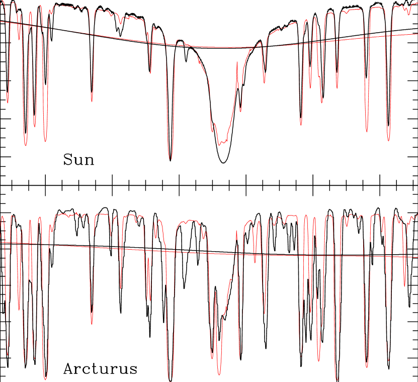
Figure 1.— The synthetic and observed spectra are compared near the region of the H$\beta$ lines. The top panel is the solar spectra and the bottom panel is Arcturus one. The thicker (black) lines are the observations. The degraded low-resolution spectra at 200 km/sec are overlaid on top of the high-resolution spectra. It is seen that the notable mismatches between the synthetic and the observed spectra at the high-resolution comparisons are smeared out at the low-resolution.

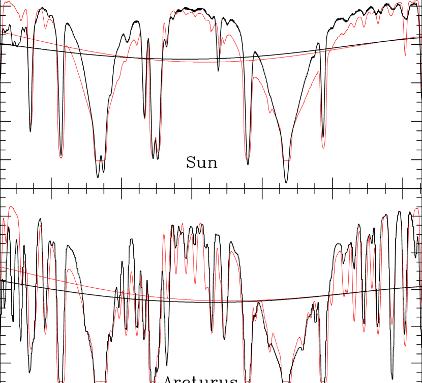
Figure 2.— Similar to Figure 1, but near the region of the Mg $b$ lines.

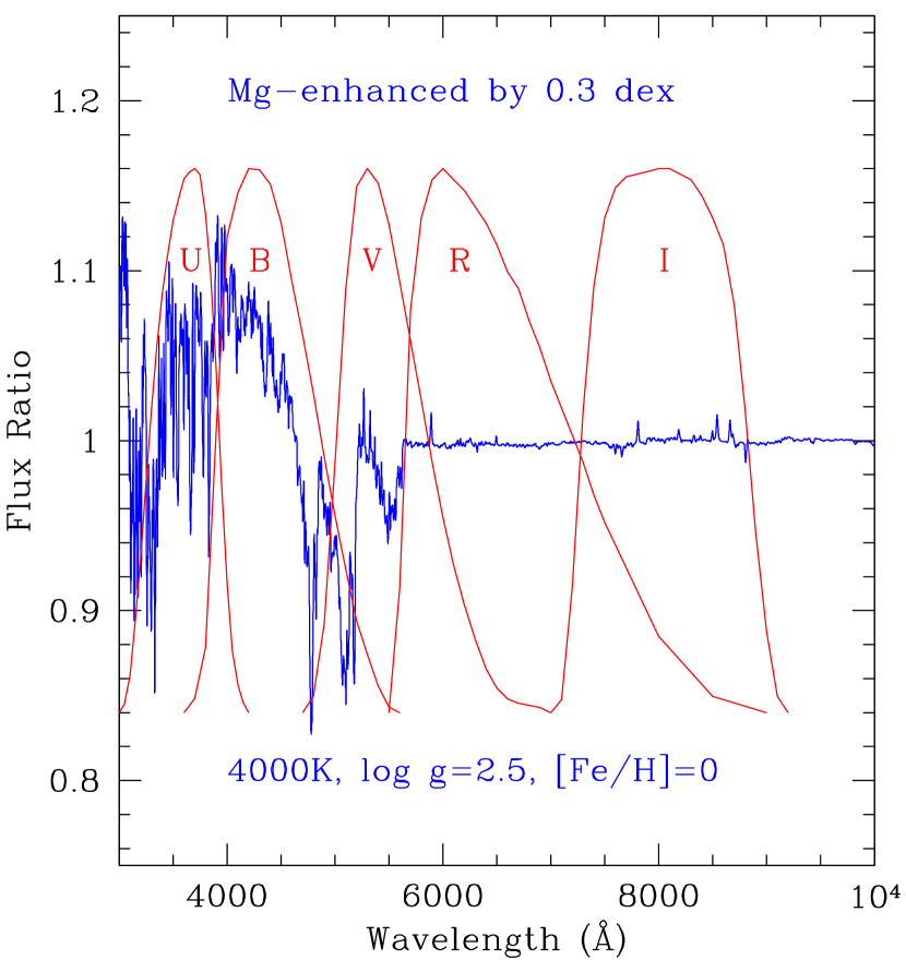
Figure 3.— At 4000 K and log g = 2.5, solar-scaled and Mg-enhanced spectra are divided. $UBVRI$-band filter response curves are overlaid. The blue colors of $U-B$ and $B-V$ and red colors of $V-R$ and $V-I$ from the Mg-enhanced spectra that we read in Table 3 are visually elucidated here.

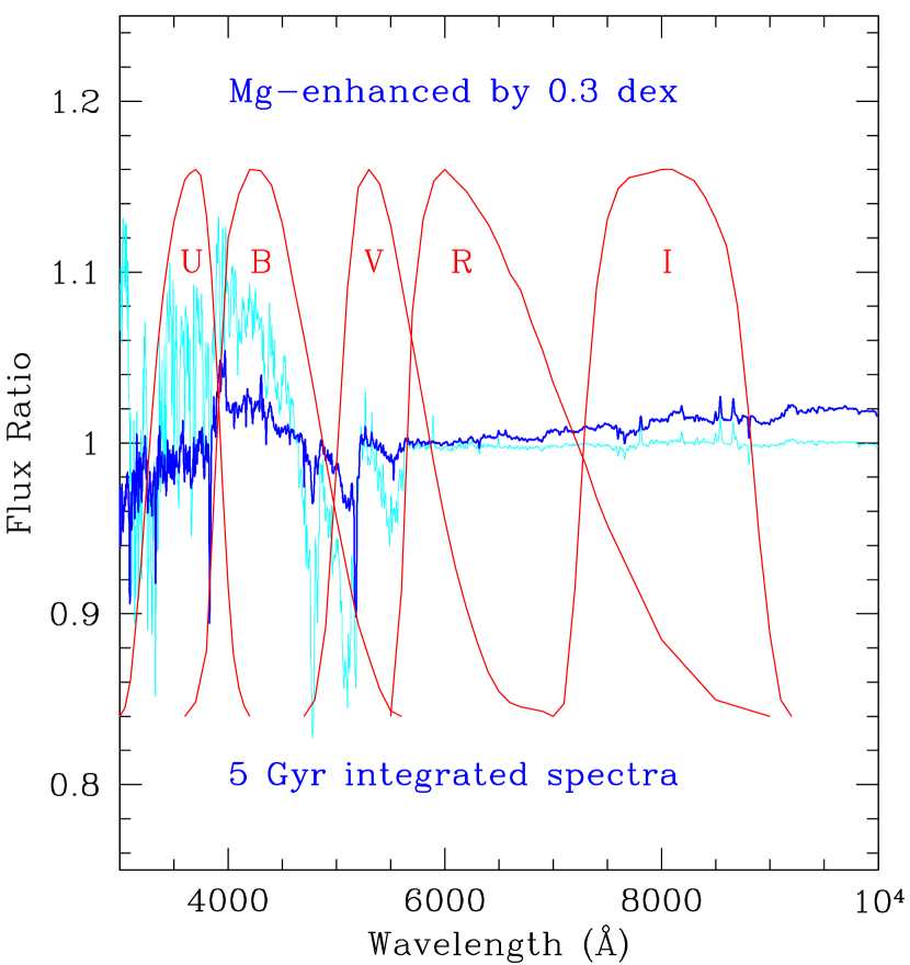
Figure 4.— Similar to Figure 3, but here the thicker line is the flux ratio between the solar-scaled and the Mg-enhanced spectra of the 5 Gyr integrated spectra at solar metallicity. It is normalized at 6000 Å. The color changes because of the Mg-enhancement that we read from Table 4 can be vividly seen here (see text).

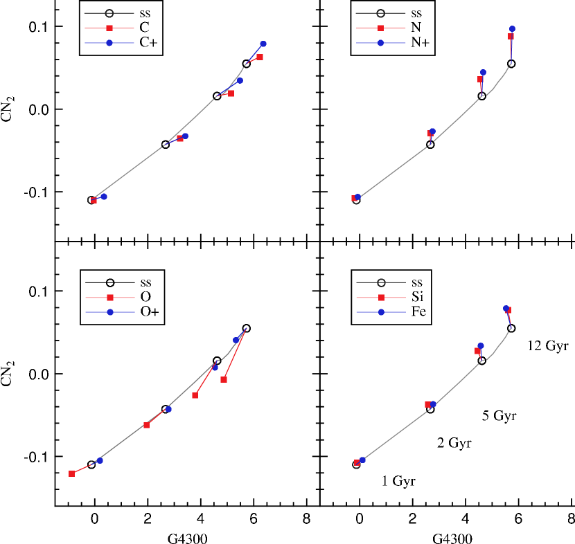
Figure 5.— CN₂ is plotted as a function of G4300 from 1 Gyr to 12 Gyr for simple stellar populations at solar metallicity. Carbon-enhanced (upper left), nitrogen-enhanced (upper right), oxygen-enhanced (lower left), and silicon-, iron-enhanced cases (lower right) at fixed $Z$ are depicted at 1, 2, 5, and 12 Gyr. C+, N+, and O+ indicate the carbon-, nitrogen-, and oxygen-enhanced cases at fixed [Fe/H], respectively.

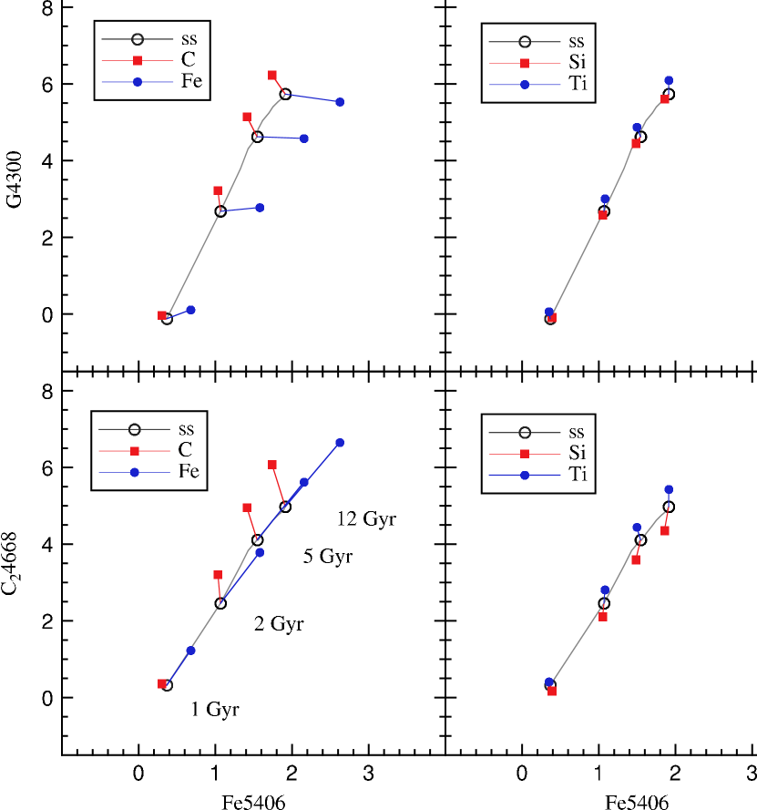
Figure 6.— Fe5406 vs. G4300 (top) and C₂4668 (bottom). Left panels show carbon- and iron-enhanced cases, while right panels display silicon- and titanium-enhanced cases. Note that C₂4668 is significantly affected both by carbon and iron. C₂4668 is further sensitive to silicon- and titanium-enhancement.

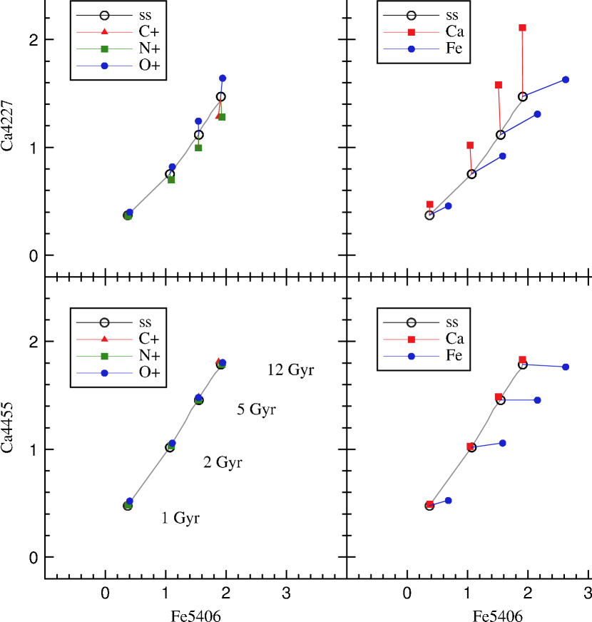
Figure 7.— Fe5406 vs. Ca4227 (top) and Ca4455 (bottom). Left panels show carbon-, nitrogen-, and oxygen-enhanced cases at fixed [Fe/H], while right panels depict calcium-, iron-enhanced cases at fixed $Z$. Ca4227 is predominantly calcium-sensitive as well as a contribution from C, N, O, and Fe, while Ca4455 is hardly altered by those elements.

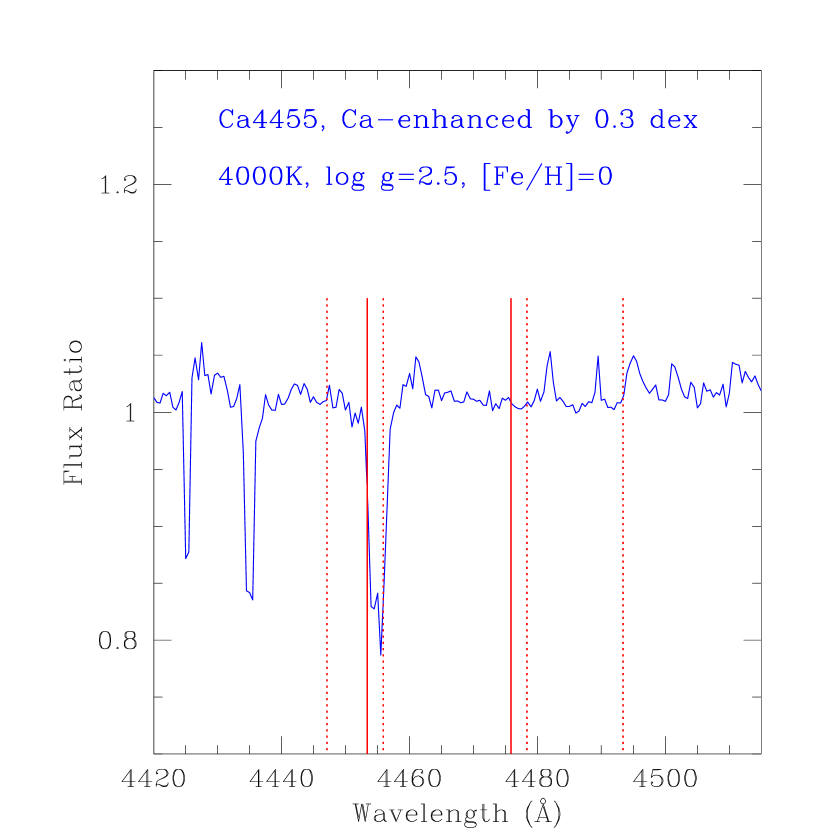
Figure 8.— At 4000 K and log g = 2.5, solar-scaled and Ca-enhanced spectra are divided. The index definition of Worthey et al. (1994) for the Ca4455 index is depicted with straight lines (solid lines for the index bandpass and dotted lines for the pseudo-continua, respectively). Note that the strong Ca line feature is shared both by the index bandpass and the blue continuum that cancel out the calcium effect on the Ca4455 index.

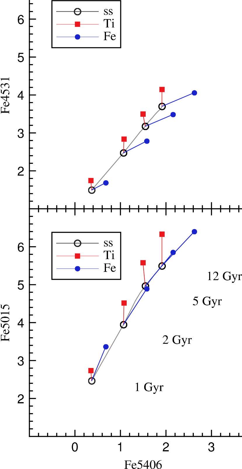
Figure 9.— Fe5406 vs. Fe4531 (top) and Fe5015 (bottom). Titanium- and iron-enhanced cases are depicted. Both of these Lick indices show a titanium sensitivity equal to that of iron.

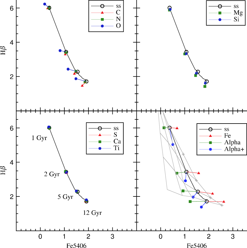
Figure 10.— Displacements are shown in diagrams of H$\beta$ as a function of Fe5406 as each chemical element is enhanced by 0.3 dex, except carbon, which is enhanced by 0.2 dex. In the lower right panel, solar-scaled chemical mixtures of [Fe/H] = $-$2.0, $-$1.0, $-$0.5, 0.0, and 0.5 are connected at 1, 2, 5, and 12 Gyr. To guide the eye, the [Fe/H] = 0.5 line is marked with plus signs at given ages. Also in the lower right panel, the $\alpha$-elements enhanced case at fixed [Fe/H] is shown (see text).

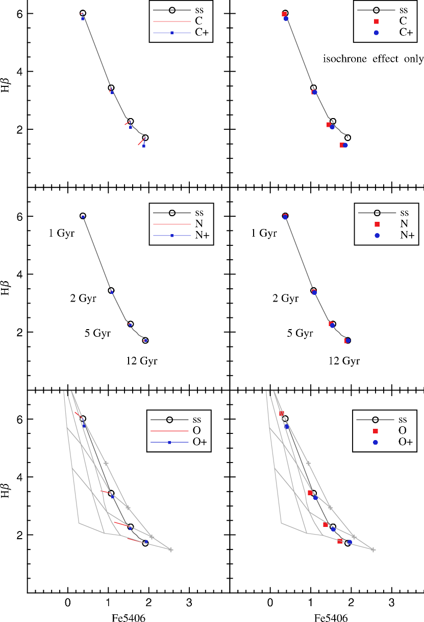
Figure 11.— C-, N-, O-enhanced cases are shown from top to bottom in diagrams of H$\beta$ as a function of Fe5406. The same solar-scaled chemical mixture grids with a range of metallicity and age are displayed here in the bottom panels as in the bottom panels of Figure 10. The left panels show the combination of isochrone and stellar spectral effects, while the right panels display the isochrone effects alone.

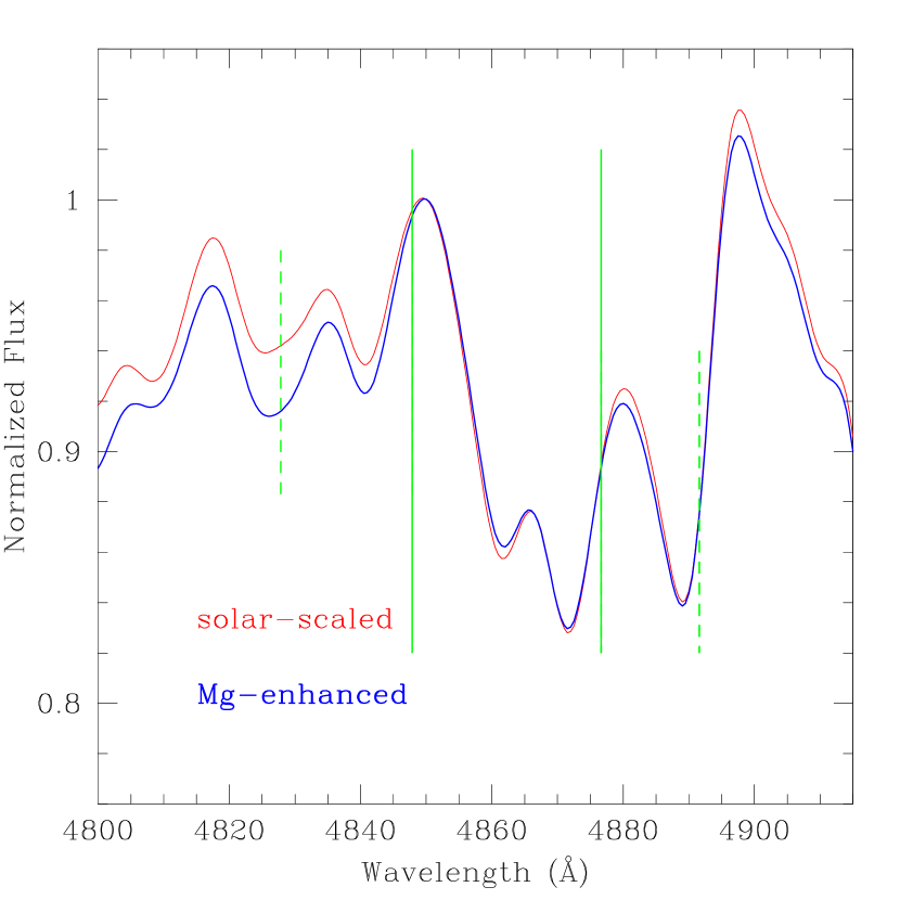
Figure 12.— Solar-scaled and Mg-enhanced 12 Gyr integrated spectra near H$\beta$ (4861 Å). Note that the Mg-lines make the blue-continuum levels significantly lower, which consequently make the H$\beta$ index strengths weaker as we see in the upper right panel of Figure 10.

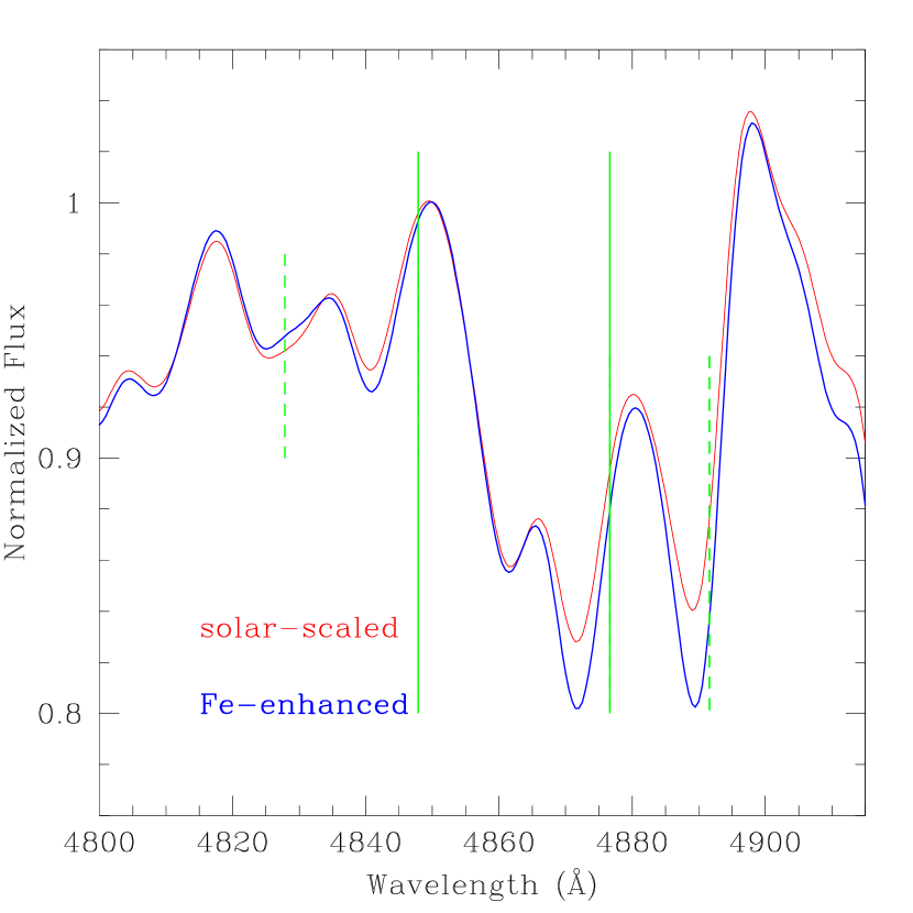
Figure 13.— Solar-scaled and Fe-enhanced 12 Gyr integrated spectra near H$\beta$ (4861 Å). Note that Fe-lines make the index bandpass and the red-continuum levels significantly lower, which consequently cancel out their effects on the H$\beta$ index strengths as we see in the lower right panel of Figure 10.

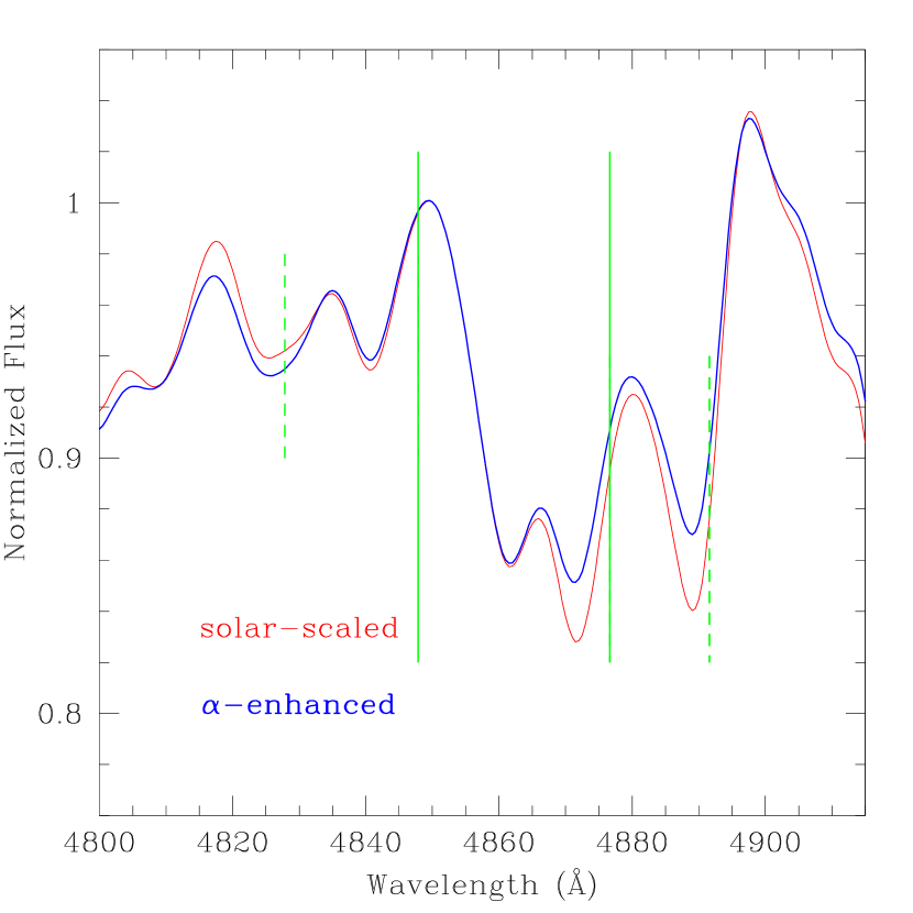
Figure 14.— Solar-scaled and the $\alpha$-enhanced 12 Gyr integrated spectra near H$\beta$ (4861 Å). Note that the $\alpha$-enhanced spectra at constant $Z$ mostly reflect the Fe depression effect which is the opposite of what is seen in Figure 13 and they affect the H$\beta$ index strengths little as we see in the lower right panel of Figure 10.

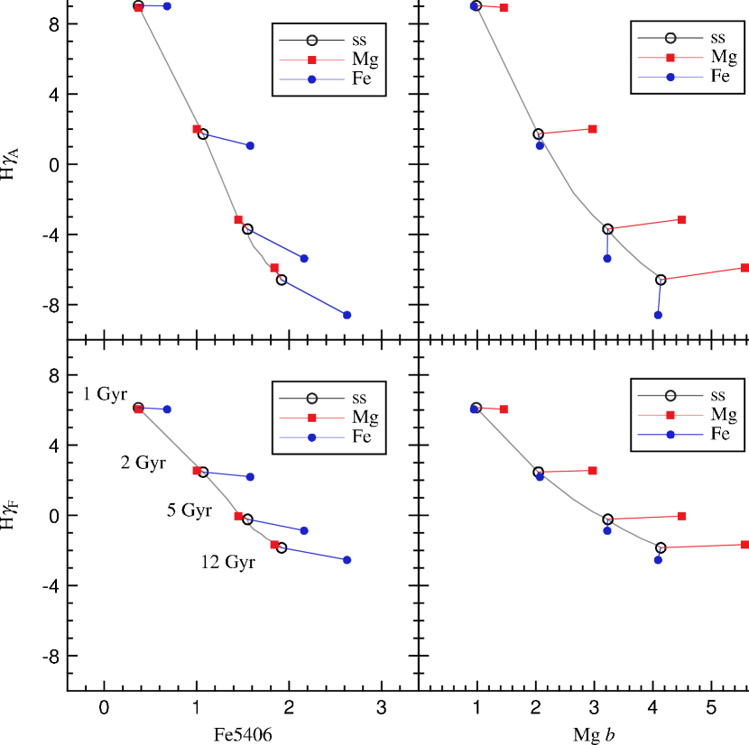
Figure 15.— H$\gamma_{A}$ (top) and H$\gamma_{F}$ (bottom) are compared with Fe5406 (left) and Mg $b$ (right). Clearly H$\gamma_{A}$ is significantly affected by iron enhancement.

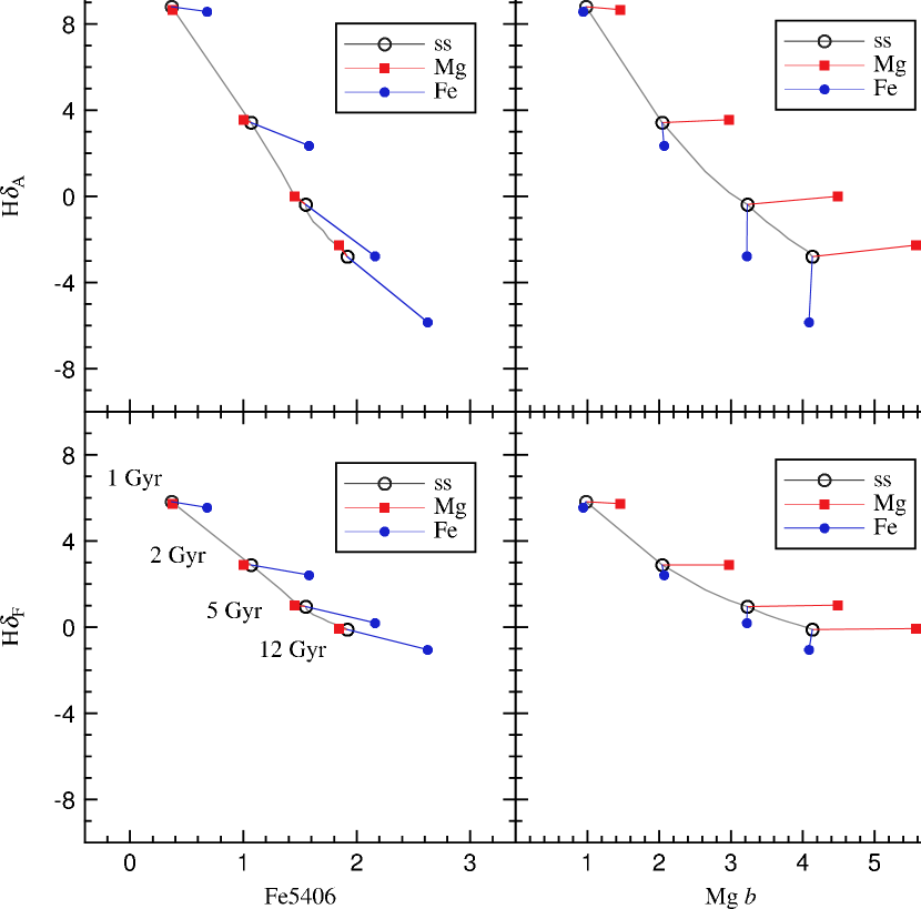
Figure 16.— Similar to Figure 15, but H$\delta_{A}$ (top) and H$\delta_{F}$ (bottom) are compared with Fe5406 (left) and Mg $b$ (right). Again, clearly H$\delta_{A}$ is significantly affected by iron enhancement.

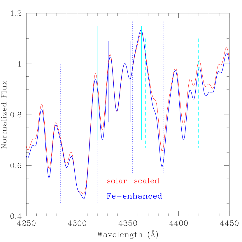
Figure 17.— Solar-scaled and Fe-enhanced 12 Gyr integrated spectra near H$\gamma$ (4341 Å). The solid lines and the dashed lines are the index bandpasses (the broader ones are the $A$ indices, while the narrower ones are the $F$ indices) and the continua regions for the $A$ indices, respectively, and the dotted lines are the continua regions for the $F$ indices. H$\gamma_{A}$ and H$\gamma_{F}$ have the same blue continuum. Note that the iron lines make the red-continuum levels significantly lower, which consequently make the H$\gamma$ index strengths weaker, especially for the broader H$\gamma_{A}$ index as we see in the upper panels of Figure 15.

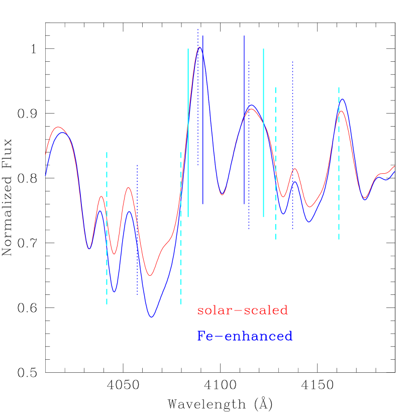
Figure 18.— Solar-scaled and Fe-enhanced 12 Gyr integrated spectra near H$\delta$ (4102 Å). Symbols are same as in Figure 17. Note that the iron lines make the continua levels significantly lower, which consequently make the H$\delta$ index strengths weaker, especially for the broader H$\delta_{A}$ index as we see in the upper panels of Figure 16.

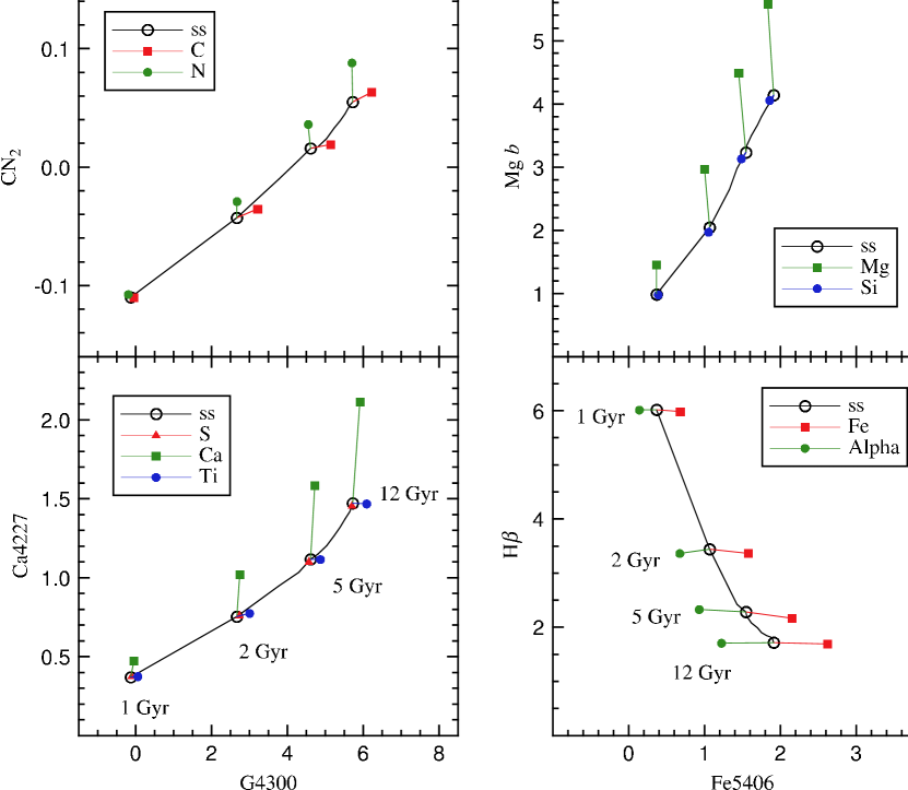
Figure 19.— The most conspicuously element-sensitive cases are collectively displayed here. Left: G4300 vs. CN₂ (top) and Ca4227 (bottom). Right: Fe5406 vs. Mg $b$ (top) and H$\beta$ (bottom).

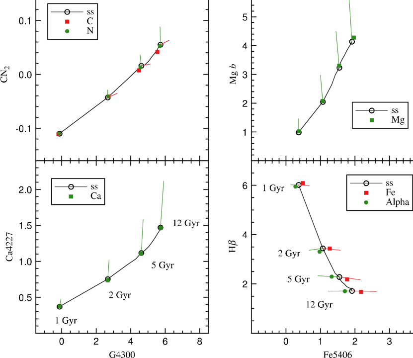
Figure 20.— Similar to Figure 19, but now filled symbols denote isochrone effects alone, while the lines show the combination of isochrone and stellar spectral effects. It is clear from this figure that stellar spectral effects dominate the changes in the indices, whereas the isochrone effects are comparatively insignificant (see text).

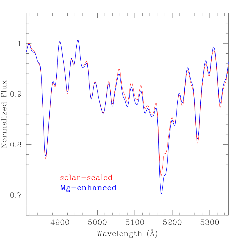
Figure 21.— 2 Gyr-old, scaled-solar spectrum smoothed to $300\,km\,s^{-1}$ compared with a 2 Gyr-old, +0.3 dex magnesium-enhanced spectrum with the same $Z$ in the SAURON spectral range. The spectra are normalized at 4750 Å. Note that Mg₁ ($\sim$ 5100 Å) and Mg $b$ ($\sim$ 5175 Å) become stronger with magnesium enhancement.

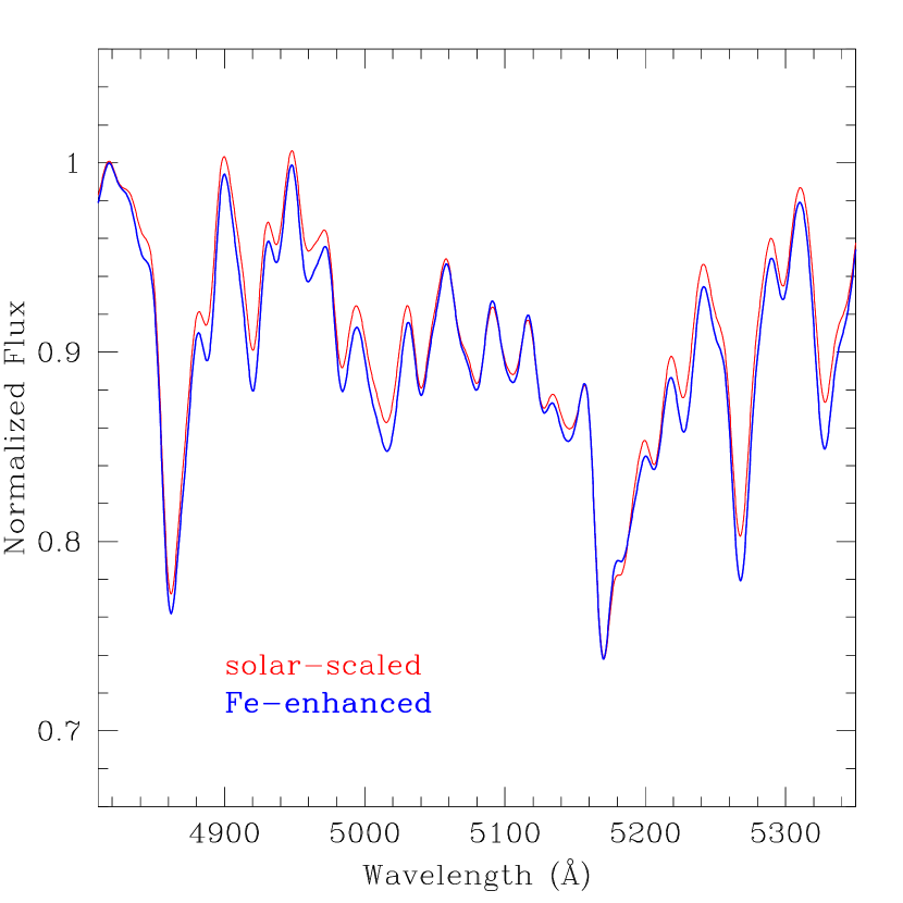
Figure 22.— 2 Gyr-old, scaled-solar spectrum smoothed to $300\,km\,s^{-1}$ compared with a 2 Gyr-old, +0.3 dex iron-enhanced spectrum with the same $Z$ in the SAURON spectral range. The spectra are normalized at 4750 Å. Note that Fe5015, Fe5270, and Fe5335 become stronger with iron enhancement.

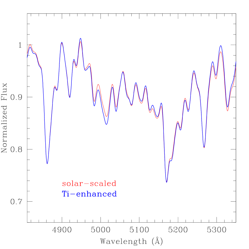
Figure 23.— 2 Gyr-old, scaled-solar spectrum smoothed to $300\,km\,s^{-1}$ compared with a 2 Gyr-old, +0.3 dex titanium-enhanced spectrum with the same $Z$ in the SAURON spectral range. The spectra are normalized at 4750 Å. Note that Fe5015 becomes stronger with titanium enhancement, while the rest of the indices are mostly intact.

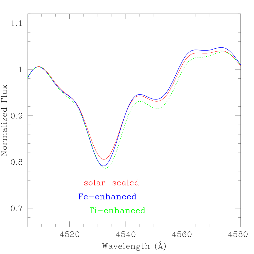
Figure 24.— Solar-scaled, Fe-enhanced, and Ti-enhanced 12 Gyr integrated spectra in the Fe4531 index region. Note that the centroids of Fe-enhanced and Ti-enhanced (dotted line) spectra are located to the left and right side of the solar-scaled one, respectively, because of different locations of Fe and Ti lines within the Fe4531 index bandpass.

References

- Bacon et al. (2001) Bacon, R. et al. 2001, MNRAS, 326, 23
- Bell et al. (1994) Bell, R. A., Paltoglou, G., & Tripicco, M. J. 1994, MNRAS, 268, 771
- Bessell (1990) Bessell, M. S. 1990, PASP, 102, 1181
- Carretta et al. (2004) Carretta, E., Gratton, R. G., Bragaglia, A., Bonifacio, P., & Pasquini, L. 2004, A&A, 416, 925
- Cassisi et al. (2004) Cassisi, S., Salaris, M., Castelli, F. & Pietrinferni. A. 2004, ApJ, 616, 498
- Cayrel et al. (1991) Cayrel, R., Perrin, M.-N., Barbuy, B., & Buser, R. 1991, A&A, 247, 108
- Charlot et al. (1996) Charlot, S., Worthey, G., & Bressan. A. 1996, ApJ, 457, 625
- Cid Fernandes et al. (2008) Cid Fernandes, R. et al. 2008, (arXiv:0802.0849)
- Coelho et al. (2005) Coelho, P., Barbuy, B., Meléndez, J., Schiavon, R. P., & Castilho, B. V. 2005, A&A, 443, 735
- Coelho et al. (2007) Coelho, P., Bruzual, G., Charlot, S., Weiss, A., Barbuy, B., & Ferguson, J.W. 2007, MNRAS, 382, 498
- Cohen, Blakeslee, & Ryzhov (1998) Cohen, J. G., Blakeslee, J. P., & Ryzhov, A. 1998, ApJ, 496, 808
- Dotter et al. (2007a) Dotter, A., Chaboyer, B., Jevremović, D., Baron, E., Ferguson, J. W., Sarajedini, A., & Anderson, J. 2007a, AJ, 134, 376
- Dotter et al. (2007b) Dotter, A., Chaboyer, B., Ferguson, J. W., Lee, H.-c., Worthey, G., Jevremović, D., & Baron, E. 2007b, ApJ, 666, 403 (Paper I)
- Ferguson et al. (2005) Ferguson, J. W., Alexander, D. R., Allard, F., Barman, T., Bodnarik, J. G., Hauschildt, P. H., Heffner-Wong, A., & Tamanai, A. 2005, ApJ, 623, 585
- Fulbright et al. (2007) Fulbright, J. P., McWilliam, A., & Rich, R. M. 2007, ApJ, 661, 1152
- Graves & Schiavon (2008) Graves, G. J., & Schiavon, R. P. 2008, (arXiv: 0803.1483)
- Gray & Brown (2001) Gray, D. F., & Brown, K. 2001, PASP, 113, 723
- Griffin & Lynas-Gray (1999) Griffin, R. E. M., & Lynas-Gray, A. E. 1999, AJ, 117, 2998
- Gustafsson et al. (1975) Gustafsson, B., Bell, R. A., Eriksson, K., & Nordlund, Å 1975, A&A, 42, 407
- Koch & McWilliam (2008) Koch, A., & McWilliam, A. 2008, AJ, 135, 1551
- Korn et al. (2005) Korn, A. J., Maraston, C., & Thomas, D. 2005, A&A, 438, 685 (KMT05)
- Kurucz (1970) Kurucz, R. L. 1970, SAO Special Report #309
- Lee & Worthey (2005) Lee, H.-c., & Worthey, G. 2005, ApJS, 160, 176 (LW05)
- Lee et al. (2007a) Lee, H.-c., Worthey, G., Trager, S. C. & Faber, S. M. 2007a, ApJ, 664, 215
- Lee et al. (2007b) Lee, H.-c., Worthey, G., Trager, S. C., Dotter, A., Chaboyer, B., Ferguson, J. W., Jevremović, D., Baron, E., Coelho, P., & Briley, M. M. 2007b, in Stellar Populations as Building Blocks of Galaxies, IAU Symposium 241, Ed. R. F. Peletier, A. Vazdekis, in press, (astro-ph/0701666)
- Mármol-Queraltó et al. (2008) Mármol-Queraltó, E., et al. 2008, A&A, in press (arXiv:0806.0581)
- Martell et al. (2008) Martell, S. L., Smith, G. H. & Briley, M. M. 2008, PASP, in press (arXiv:0806.0012)
- Martins & Coelho (2007) Martins, L. P., & Coelho, P. 2007, MNRAS, 381, 1329
- Milone et al. (2000) Milone, A., Barbuy, B., & Schiavon, R. P. 2000, AJ, 120, 131
- Ocvirk et al. (2006) Ocvirk, P., Pichon, C., Lancon, A., & Thiebaut, E. 2006, MNRAS, 365, 74
- Panter et al. (2007) Panter, B., Jimenez, R., Heavens, A. F., & Charlot, S. 2007, MNRAS, 378, 1550
- Peterson et al. (1993) Peterson, R. C., Dalle Ore, C. M., & Kurucz, R. L. 1993, ApJ, 404, 333
- Plez (1992) Plez, B. 1992, A&AS, 94, 527
- Prochaska et al. (2005) Prochaska, L. C., Rose, J. A., & Schiavon, R. P. 2005, AJ, 130, 2666
- Prochaska et al. (2007) Prochaska, L. C., Rose, J. A., Caldwell, N., Castilho, B. V., Concannon, K., Harding, P., Morrison, H., & Schiavon, R. P. 2007, AJ, 134, 321
- Proctor & Sansom (2002) Proctor, R. N., & Sansom, A. E. 2002, MNRAS, 333, 517
- Puzia et al. (2002) Puzia, T. H., et al. 2002, A&A, 395, 45
- Salasnich et al. (2000) Salasnich, B., Girardi, L., Weiss, A., & Chiosi, C. 2000, A&A, 361, 1023
- Salpeter (1955) Salpeter, E. E. 1955, ApJ, 121, 161
- Schiavon (2007) Schiavon, R. P. 2007, ApJS, 171, 146
- Schiavon et al. (2002) Schiavon, R. P., Faber, S. M., Castilho, B. V., & Rose, J. A. 2002, ApJ, 580, 850
- Serven et al. (2005) Serven, J.L., Worthey, G., & Briley, M. M. 2005, ApJ, 627, 754
- Thomas & Maraston (2003) Thomas, D., & Maraston, C. 2003, A&A, 401, 429
- Thomas et al. (2003) Thomas, D., Maraston, C., & Bender, R. 2003, MNRAS, 339, 897
- Thomas et al. (2004) Thomas, D., Maraston, C., & Korn, A. J. 2004, MNRAS, 351, L19
- Trager (1997) Trager, S. C. 1997, Ph.D. thesis, Univ. California, Santa Cruz
- Trager et al. (2000a) Trager, S. C., Faber, S. M., Worthey, G., González, J. J. 2000a, AJ, 119, 1645
- Trager et al. (2000b) Trager, S. C., Faber, S. M., Worthey, G., González, J. J. 2000b, AJ, 120, 188
- Tripicco & Bell (1995) Tripicco. M. J., & Bell, R. A. 1995, AJ, 110, 3035 (TB95)
- Vazdekis (1999) Vazdekis, A. 1999, ApJ, 513, 224
- Weiss et al. (2006) Weiss, A., Salaris, M., Ferguson, J. W., & Alexander, D. R. 2006, (astro-ph/0605666)
- Worthey (1994) Worthey, G. 1994, ApJS, 95, 107
- Worthey (1998) Worthey, G. 1998, PASP, 110, 888
- Worthey et al. (1994) Worthey, G., Faber, S. M., González, J. J., & Burstein, D. 1994, ApJS, 94, 687
- Worthey & Lee (2008) Worthey, G., & Lee, H.-c. 2008, ApJS, submitted (astro-ph/0604590)
- Worthey & Ottaviani (1997) Worthey, G., & Ottaviani, D. L. 1997, ApJS, 111, 377
- Yong et al. (2008) Yong, D., Grundahl, F., Johnson, J. A. & Asplund, M. 2008, ApJ, in press (arXiv:0806.0187)