On the jet contribution to the AGN cosmic energy budget

Abstract

Black holes release energy via the production of photons in their accretion discs but also via the acceleration of jets. We investigate the relative importance of these two paths over cosmic time by determining the mechanical luminosity function (LF) of radio sources and by comparing it to a previous determination of the bolometric LF of active galactic nuclei (AGN) from X-ray, optical and infrared observations. The mechanical LF of radio sources is computed in two steps: the determination of the mechanical luminosity as a function of the radio luminosity and its convolution with the radio LF of radio sources. Even with the large uncertainty deriving from the former, we can conclude that the contribution of jets is unlikely to be much larger than $\sim 10\%$ of the AGN energy budget at any cosmic epoch.

1 Introduction

Matter can accrete onto a black hole (BH) only if it releases a fraction $\epsilon\sim 0.06-0.4$ of its rest-mass energy, where $\epsilon$ depends on the BH spin (Bardeen, 1970). In the standard Shakura & Syunyaev (1973) model, the energy is dissipated by viscous torques in the accretion disc and radiated. Accretion from a luminous disc provides a physical model to explain the luminosity of quasars (Lynden-Bell, 1969).

Several authors have computed the total energy radiated by BHs over cosmic time and have compared it to the local BH mass density (Soltan, 1982; Chokshi & Turner, 1992; Yu & Tremaine, 2002; Barger et al., 2005; Hopkins et al., 2007). The two are in good agreement if matter is turned into light with a canonical efficiency of $\epsilon\sim 0.1$. This has been used as an argument to infer that most of the BH mass in the Universe was accreted luminously, but it only proves that $>25\%$ of the BH mass in the Universe was accreted luminously, since $\epsilon$ could be as large as $\epsilon\sim 0.4$ if most BHs were maximally rotating.

In fact, accreting BHs (‘active galactic nuclei’, AGN) produce not only light but also jets of matter, which are radio-luminous because of the synchrotron radiation from ultrarelativistic electrons accelerated in shocks. Excluding objects beamed toward the line of sight, only a small fraction of the luminosity that is radiated by an AGN comes from synchrotron radiation. However, the synchrotron power represents only a small fraction of the jet mechanical luminosity, most of which may be used to do work on the surrounding gas.

Moreover, at low accretion rates ($\dot{M}_{\bullet}\lower 2.15277pt\hbox{$\;\buildrel<\over{\sim}\;$}0.01\dot{M}_{\rm Edd}$, where $L_{\rm Edd}=\epsilon\dot{M}_{\rm Edd}{\rm c}^{2}$ is the Eddington luminosity), the accretion disc is not dense enough to radiate efficiently; the disc puffs up, and the energy that needs to be removed to allow the accretion may be carried out more easily by jets. Although the physics of this picture are still speculative, AGN that channel a large fraction of the accretion power into jets while showing little emission from an accretion disc are observed (eg Di Matteo et al., 2003; Allen et al., 2006). These radio sources are less powerful than quasars but more common due to their longer duty cycle. For example, around two-thirds of brightest cluster galaxies are radio galaxies (Burns, 1990; Best et al., 2007). In contrast, only one galaxy in $10^{4}$ contains a quasar ($M_{B}<-23$) at $z\sim 0$ (Wisotzki et al., 2001). Finally, mechanical energy is thermalized in the intracluster medium more efficiently than luminous energy is. The observational evidence that the mechanical heating by AGN is important to solve the cooling-flow problem in galaxy groups and clusters is getting strong (Best et al., 2005a; Dunn & Fabian, 2006; Rafferty et al., 2006; Magliocchetti & Brüggen, 2007; see also Cattaneo et al. 2009, and references therein).

For these reasons, it is important to compare the mechanical and radiative output of AGN. This is the goal of the current paper. This issue has also recently been addressed by Shankar et al. (2008a), Körding et al. (2008) and Merloni & Heinz (2008). We adopt a different approach to these authors and produce results that are qualitatively similar. The layout of our paper is as follows. In Section 2, we analyse how we can use radio data to infer the jet mechanical power. We shall see that two different approaches give different $P_{\rm jet}(L_{\rm radio})$ relations. We consider both, and use the difference between the results obtained from the two relations to provide an estimate of the uncertainty. We convolve these relations with the radio LF of radio sources, $\phi(L_{\rm radio})$, to estimate the mechanical LF, $\phi(L_{\rm radio}(P_{\rm jet}))$, first in the local Universe (Section 3), then at different redshifts (Section 4). In both cases, we integrate over luminosity to determine the mechanical power per unit volume, which we compare with the radiative power per unit volume from luminous AGN. In Section 5 we summarize the results of comparing the mechanical LF of AGN to the bolometric luminosity function of AGN determined by Hopkins et al. (2007) and we discuss the implications of our results.

2 The mechanical luminosity of a radio source

Obtaining an estimate of the mechanical power of a radio source is an inherently difficult problem. The observed monochromatic radio luminosity measures only the fraction of the jet power that is currently being converted into radiation. That fraction is small (typically between 0.1 and $1\%$; cf. Bicknell, 1995) and changes during the lifetime of the radio source, since the radio luminosity of a growing radio source first increases and then drops as the source expands into a progressively lower density environment (eg Kaiser et al., 1997). Nevertheless, it is reasonable to expect that radio and mechanical luminosities should show at least a broad degree of correlation on a population basis.

Estimates of the mechanical power of radio sources have followed two approaches. The first (Willott et al., 1999) uses the minimum energy density $u_{\rm min}$ that the plasma in the radio lobes must have in order to emit the observed synchrotron radiation (eg Miley, 1980). With this approach, the jet mechanical power is $L_{\rm mech}\lower 2.15277pt\hbox{$\;\buildrel>\over{\sim}\;$}u_{\rm min}V/t$, where $V$ is the volume filled by the radio lobes and the radio-source lifetime $t$ is given by the ratio between the jets’ length and the hotspots’ advancement speed. The largest sources of uncertainties are: (i) the nature of the jet plasma (electron-positron or electron-proton?): the value of $u_{\rm min}$ is larger if the lobes contain a hadronic component in addition to the synchrotron radiating particles (relativistic electrons and/or positrons); (ii) the lack of observational constraints on the low-frequency cut-off of the electron energy distribution: for a synchrotrom spectrum $\propto\nu^{\alpha}$ with radio spectral index $\alpha<-0.5$, $u_{\rm min}$ is larger when the lower cut-off frequency takes a lower value and thus there is more energy in the synchrotron spectrum. Willott et al. (1999) derive the relation

$$L_{\rm mech}=3\times 10^{38}f_{\rm W}^{3/2}\left(\frac{L_{\rm 151\,MHz}}{10^{28}{\rm W\,Hz}^{-1}{\rm sr}^{-1}}\right)^{6/7}{\rm W},$$ (1)

where $f_{W}\sim 1-20$ incorporates all the unknown factors. Blundell & Rawlings (2000) argue for $f_{\rm W}\simeq 10$ for Fanaroff & Riley (1974) class II sources (FR IIs), while Hardcastle et al. (2007) suggest $f_{\rm W}=10-20$ for FR Is. We convert the luminosity at 151 MHz, $L_{\rm 151\,MHz}$, into a luminosity at 1.4 GHz, $L_{\rm 1.4\,GHz}$, where the local radio LF is best-determined. This will also allow us later to compare Eq. (1) with another determination of $L_{\rm mech}$ by Best et al. (2006, 2007). For the conversion we assume a spectral index $\alpha=-0.8$. Using $f_{\rm W}=10$, Eq. (1) gives:

$$L_{\rm mech}=1.4\times 10^{37}\left(\frac{L_{\rm 1.4\,GHz}}{10^{25}{\rm W\,Hz}^{-1}}\right)^{0.85}{\rm W}.$$ (2)

Notice that $L_{\rm 151\,MHz}$ is given in ${\rm W\,Hz}^{-1}{\rm sr}^{-1}$ while $L_{\rm 1.4\,GHz}$ is given in ${\rm W\,Hz}^{-1}$ to respect the different conventions used by Willott et al. (1999) and Best et al. (2006), so there is a factor of $4\pi$ entering the conversion.

A second approach is to infer $L_{\rm mech}$ from the mechanical work that the lobes do on the surrounding hot gas. The expanding lobes of relativistic synchrotron-emitting plasma open cavities in the ambient thermal X-ray emitting plasma, which advances in X-ray imaging capabilities now allow to be imaged in detail. The minimum work in inflating these cavities is done for reversible (quasi-static) inflation and equals $pV$, where $p$ is the pressure of the ambient gas. Best et al. (2006) derived a relation between radio and mechanical luminosity based upon this estimate for the energy associated with these cavities, combined with an estimate of the cavity ages from the buoyancy timescale (from Bîrzan et al., 2004). Comparing the mechanical luminosities of 19 nearby radio sources that have associated X-ray cavities with their 1.4 GHz monochromatic radio luminosities leads to a relation

$$L_{\rm mech}=(3.0\pm 0.2)\times 10^{36}\,f\,\left(\frac{L_{\rm 1.4\,GHz}}{10^{25}{\rm W\,Hz}^{-1}}\right)^{0.40\pm 0.13}{\rm W},$$ (3)

broadly in agreement with that derived by Bîrzan et al. (2004). In Eq. (3), the factor $f$, incorporated by Best et al. (2007), accounts for any systematic error in estimating the mechanical luminosities of the cavities. In particular, $pV$ is likely to be an underestimate of the energy needed to inflate a cavity: the enthalpy of the cavity is $\frac{\gamma}{\gamma-1}pV=4pV$ for the relativistic plasma in the radio lobes, suggesting that $f\sim 4$ may be appropriate. Some authors have even argued for mechanical energies in excess of $10pV$ (Nusser et al., 2006; Binney et al., 2007) due to additional heating directly from the jets. For $f=4$, Eq. (3) gives:

$$L_{\rm mech}=1.2\times 10^{37}\left(\frac{L_{\rm 1.4\,GHz}}{10^{25}{\rm W\,Hz}^{-1}}\right)^{0.40}{\rm W}.$$ (4)

Eqs. 2 and 4 are in excellent agreement at $L_{\rm 1.4\,GHz}\sim 10^{25}{\rm W\,Hz}^{-1}$, but the relation derived from the minimum-energy argument has a steeper radio luminosity dependence than the relation derived from the X-ray cavities. Nevertheless, given the totally independent approaches used to derive Eqs. 2 and 4, and the uncertainty factors in both equations, the degree of consistency is encouraging. Indeed, the discrepency between the two relations may simply reflect the fact that Eq. 2 is determined from powerful, radiatively efficient radio sources (mostly $L_{\rm 1.4\,GHz}\lower 2.15277pt\hbox{$\;\buildrel>\over{\sim}\;$}10^{25}{\rm W\,Hz}^{-1}$) while Eq. 4 is derived predominantly from lower luminosity, radiatively inefficient sources. The mean relation between $L_{\rm mech}$ and $L_{\rm rad}$ may well be different in these two different regimes, in which case a combination of Eq. 2 at high luminosities and Eq. 4 at low luminosities would be most appropriate.

A third approach towards estimating mechanical luminosities of radio sources has been developed by Merloni & Heinz (2008). These authors use the de-beamed radio core emission as a measure of the jet kinetic luminosity, based upon the analogy with X-ray binary sources and the so-called Fundamental Plane relation for black holes (Merloni et al., 2003). This approach uses the radio LF of flat-spectrum (ie core-dominated) radio sources as a measure of the LF of radio cores. It then requires assumptions about the statistical de-beaming of radio sources (ie the distribution of Lorentz factors of jets), and about how to correct for the radio cores that are missed from the flat-spectrum radio LF because their radio sources are dominated by extended steep spectrum emission. These factors can be reasonably estimated for moderate to high radio luminosity sources in the local Universe, but they are not so well constrained at low radio luminosities, where the bulk of the jet mechanical power is produced, nor at higher redshifts. We therefore do not consider this approach here, but we do compare our results with the results obtained by Merloni & Heinz (2008) in Section 5.

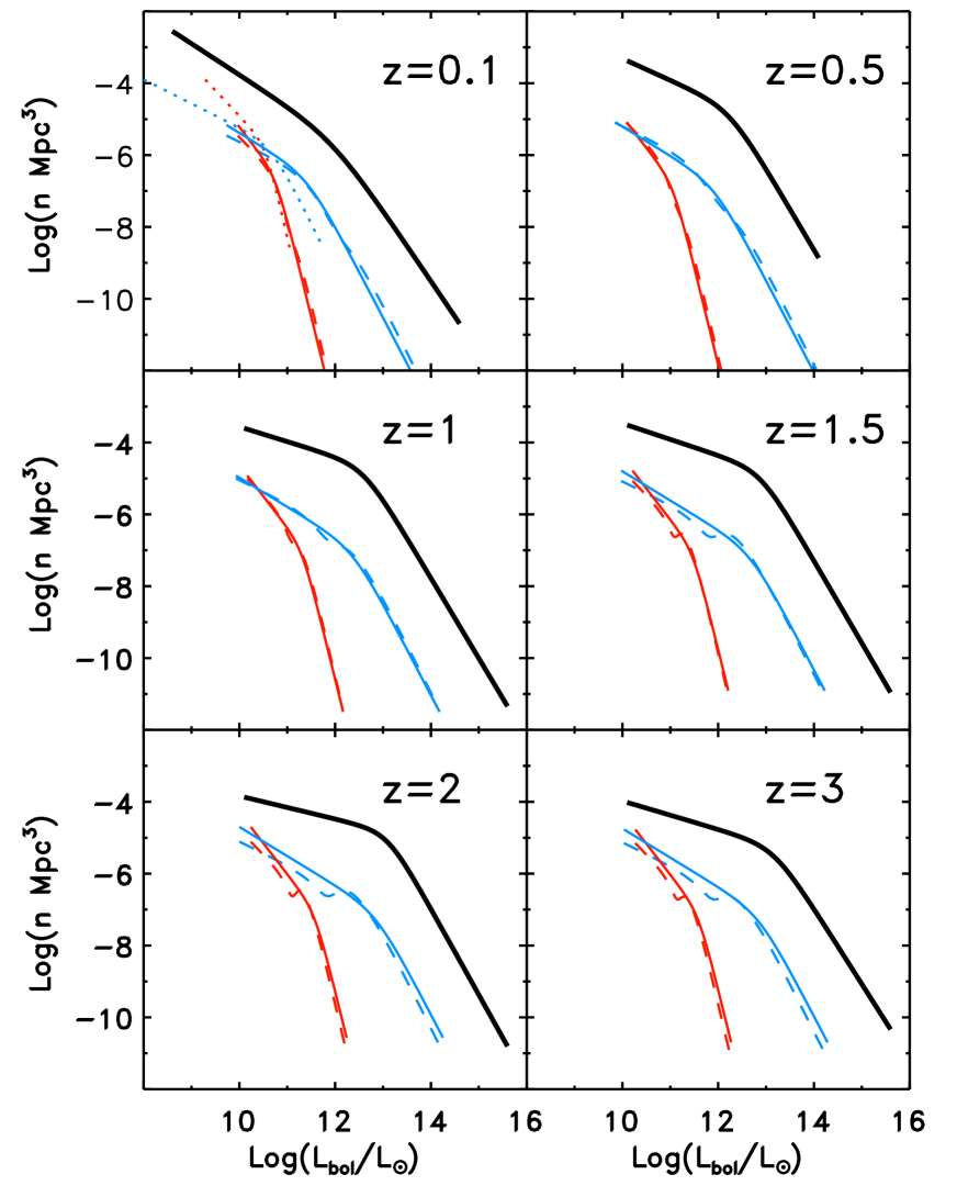
Figure 1: The thick solid lines show the bolometric LF of AGN inferred by Hopkins et al. (2007) from X-ray, optical and infrared data. The thin solid and dashed lines show the mechanical LFs inferred from the radio LFs of Dunlop & Peacock (1990) and Willott et al. (2001), respectively. At $z\simeq 0$, we have also shown the mechanical LFs inferred from Best et al. (2005b)’s local radio LF (dotted lines). For each radio LF, we have determined two mechanical LFs, according to the two different $P_{\rm jet}(L_{\rm radio})$ conversions derived in Section 2: the red lines are for $P_{\rm jet}\propto L_{\rm radio}^{0.4}$ (Eq. 4) and the blue lines are for $P_{\rm jet}\propto L_{\rm radio}^{0.85}$ (Eq. 2).

3 The local mechanical LF

In order to derive a mechanical LF for radio sources in the nearby Universe, we must convolve Eqs. 2 and 4 with the local radio LF. Here we adopt the local 1.4 GHz radio LF of Best et al. (2005a), which is derived from the Sloan Digital Sky Survey spectroscopic sample and is fully consistent with other recent determinations of the local radio LF (eg Machalski & Godlowski, 2000; Sadler et al., 2002). Throughout this paper we follow the convention of defining the LF $\phi(L)$ as the number of objects per unit volume and logarithmic-luminosity interval (eg Hopkins et al., 2007), so the number of sources with luminosity between $L$ and $L+{\rm d}L$ is $(\phi/{\rm ln}10){\rm d}L/L$. With this definition, the Best et al. (2005a) LF can be be parameterised using the double power-law model

$$\phi(L)=\phi_{*}\left[\left(\frac{L}{L_{*}}\right)^{\alpha}+\left(\frac{L}{L_{*}}\right)^{\beta}\right]^{-1},$$ (5)

where $L=L_{\rm 1.4\,GHz}$ (we wrote $L$ without any subscripts because we shall use Eq. 5 to model other LFs). The best-fit parameters are $\phi_{*}=10^{-5.7}$Mpc^-3, $L_{*}=10^{25.16}$W Hz^-1, $\alpha=0.57$ and $\beta=2.31$. Combining Eq. (5) with Eqs. 2 and 4 gives the blue and the red dotted curves in the $z=0.1$ diagram of Fig. 1, respectively.

The mechanical power that is released per unit volume is

$$\rho_{\rm mech}=\int_{0}^{\infty}L_{\rm mech}(L){\phi(L)\over{\rm ln}10}{{\rm d}L\over L}$$ (6)

$$=A\left({L\over 10^{25}{\rm\,W}}\right)^{\eta}\int_{0}^{\infty}{{\rm d}x\over x^{\alpha+1-\eta}+x^{\beta+1-\eta}},$$

where $A=4.8\times 10^{11}L_{\odot}$ and $\eta=0.85$ for Eq. (2), and $A=1.0\times 10^{11}L_{\odot}$ and $\eta=0.4$ for Eq. (4). If $L_{\rm mech}$ is computed with Eq. (2), then $\rho_{\rm mech}^{\rm synchro}=1.6\times 10^{5}L_{\odot}{\rm\,Mpc}^{-3}$ ($1L_{\odot}=3.9\times 10^{26}{\rm\,W}$). If $L_{\rm mech}$ is computed with Eq. (4), the problem is more complicated because in that case the integral in Eq. (6) diverges at $x=0$. This is because the double power-law model in Eq. (5) cannot be extrapolated down to $L\rightarrow 0$, as can be easily seen: the faint-end slope of the local radio LF is steeper than that of both the low luminosity end of the local galaxy optical LF (eg Norberg et al., 2002) and the low mass end of the local mass function of supermassive black holes (eg Shankar et al., 2008b). Therefore, if the radio LF extrapolated too far, then the calculated space density of radio-loud AGN would exceed that of galaxies (or supermassive black holes) capable of hosting them. For example, if the slope of the radio LF were to remain unaltered down to $L_{\rm 1.4\,GHz}=10^{17}{\rm W\,Hz}^{-1}$ then the local space density of radio galaxies would exceed that of galaxies integrated down to $M_{B}\sim-15$.

Considering that only massive galaxies with massive black holes have a significant probability of harbouring a radio source powered by an AGN, the local space density of radio sources matches that of supermassive black holes with $M_{\bullet}\lower 2.15277pt\hbox{$\;\buildrel>\over{\sim}\;$}10^{6}M_{\odot}$ (ie $\sim 5\times 10^{-3}{\rm\,Mpc}^{-3}$ according to Shankar et al., 2008b) if the radio LF is extrapolated down to $L_{\rm 1.4\,GHz}\sim 10^{19.2}{\rm W\,Hz}^{-1}$. This sets a strong lower limit on the luminosity to which the radio LF can be extrapolated, and so for a conservative calculation we evaluate the integral in Eq. (6) by adopting $10^{19.2}{\rm W\,Hz}^{-1}/L_{*}\simeq 10^{-6}$ as the lower extreme of the integration interval. With this choice, the mechanical power per unit volume from Eq. (4), $\rho_{\rm mech}^{\rm cav}$, is about ten times larger than the mechanical power per unit volume from Eq. (2), $\rho_{\rm mech}^{\rm synchro}$. The discrepency would reduce to a factor of three if a limit of $10^{22}{\rm W\,Hz}^{-1}$ were adopted instead.

We want to compare these values to the radiative power per unit volume from luminous AGN. Hopkins et al. (2007) made the first attempt at determining the bolometric LF of AGN by combining hard X-ray, soft X-ray, optical and infrared data. They found that the double power-law model in Eq. (5) fits their results with $\phi_{*}$, $L_{*}$, $\alpha$ and $\beta$ dependent on redshift (here $L$ is the bolometric luminosity $L_{\rm bol}$, not the radio luminosity). The thick solid lines in Fig. 1 show their best fit at different $z$. We use their best fit to the bolometric LF at $z=0.1$ to estimate the power per unit volume radiated by AGN in the local Universe:

$$\rho_{\rm rad}=\int_{0}^{\infty}L_{\rm bol}{\phi(L_{\rm bol})\over{\rm ln}10}{{\rm d}L_{\rm bol}\over L_{\rm bol}}.$$ (7)

We find that $\rho_{\rm mech}^{\rm synchro}/\rho_{\rm rad}\simeq 0.018$ (the level of the dashed line in Fig. 2). The value of $\rho_{\rm mech}^{\rm cav}/\rho_{\rm rad}$ depends on the radio luminosity $L_{\rm min}$ that is taken for the lower bound of the integration interval in Eq. (6) (solid line in Fig. 2). For $L_{\rm min}/L_{*}\simeq 10^{-6}$, $\rho_{\rm mech}^{\rm cav}/\rho_{\rm rad}\simeq 0.2$. For $\rho_{\rm mech}^{\rm cav}$ to be comparable to $\rho_{\rm rad}$, the power law of the radio LF would have to extrapolate down to $L_{\rm 1.4\,GHz}=10^{15}{\rm W\,Hz}^{-1}$ (Fig. 2), which is well below the allowed limits.

Figure 2: The ratio between the mechanical power of radio sources (Eq. 6) and the radiative power of luminous AGN (Eq. 7) in a representative volume of the local Universe. The solid line is computed using the mechanical power estimated from the size of the X-ray cavities (Eq. 4), in which case $\rho_{\rm mech}$ depends on the minimum luminosity $L_{\rm min}$ at which one can extrapolate the LF in Eq. (5). The dashed line is computed using the mechanical power estimated from the minimum energy that is needed to explain the observed synchrotron emission (Eq. 2), in which case $\rho_{\rm mech}$ does not depend on this uncertainty. Both lines are computed using the local LF of Best et al. (2005a). The vertical dotted line is a conservative lower limit for $L_{\rm min}$.

4 The evolution of the mechanical LF

To go beyond the local Universe, we need to know the evolution of the radio LF with redshift (assuming that there is no redshift dependence in Eqs. 2 and 4). We use the radio LFs determined by Dunlop & Peacock (1990) and Willott et al. (2001).

Dunlop & Peacock (1990) modelled the 2.7 GHz LF with the sum of three contributions: steep-spectrum radio sources in early-type galaxies, flat-spectrum radio sources in early-type galaxies, and radio sources in late-type galaxies. The latter are mainly powered by star formation and are thus irrelevant for our analysis. Flat-spectrum radio sources are beamed (the jets are aligned with the line of sight); therefore, the equations in Section 2 overestimate their mechanical luminosity. The addition of the LF of flat-spectrum radio sources to that of steep-spectrum radio sources makes little difference to the latter, and so it is safe to deal with this complication by considering only steep-spectrum radio sources. The 2.7 GHz LF of steep-spectrum radio sources in early-type galaxies computed by Dunlop & Peacock (1990) is a double power-law function of the form of Eq. (5). In their pure luminosity evolution model (their other models give similar LFs out to $z\sim 2$) the dependence of redshift is entirely contained in $L_{*}=10^{24.89+1.26z-0.26z^{2}}{\rm W\,Hz}^{-1}{\rm sr}^{-1}$. We take this LF, convert it into a 1.4 GHz LF by assuming an $\alpha=-0.8$ spectral index, and correct for a cosmology with $\Omega_{M}=0.3$, $\Omega_{\Lambda}=0.7$ and $h=0.7$ so that we can compare our results with the bolometric LF determined by Hopkins et al. (2007), since Dunlop & Peacock (1990) had assumed $\Omega_{M}=1$, $\Omega_{\Lambda}=0$ and $h=0.5$. The blue and red solid lines in Fig. 1 are obtained by convolving the 1.4 GHz LF determined in this manner with Eqs. 2 and 4, respectively. Both the blue and the red curves are significantly below the bolometric LF estimated by Hopkins et al. (2007; thick solid lines) at all redshifts.

To check this result with an independent determination of the radio LF, we consider Willott et al. (2001)’s best fit to the 151 MHz LF (their model C). We transform it into a 1.4 GHz LF by assuming $\alpha=-0.8$ and correct for the cosmology (Willot et al. 2001 had assumed the same cosmology as Dunlop & Peacock 1990). The blue and the red dashed lines in Fig. 1 are obtained by convolving the 1.4 GHz LF determined in this manner with Eqs. 2 and 4, respectively. The dashed lines and the thin solid lines of the same colour run very close to each other. This demonstrates that the radio LF is not a major source of uncertainty when it comes to determining the mechanical LF of AGN, even at high redshifts.

The mechanical power per unit volume obtained integrating Eq. (2) over the LF of Dunlop & Peacock (1990), $\rho_{\rm mech}^{\rm synchro}$, is shown as a function of redshift in Fig. 3 (dashed line) and compared to the radiative power per unit volume from Eq. (7) (symbols). The dotted line in Fig. 3 is simply $57\rho_{\rm mech}^{\rm synchro}$. It shows that the cosmic evolution of the mechanical power density traces that of the radiative power density, at least for Eq. (2). It also shows that throughout cosmic time jets contribute to a small fraction ($\sim 2\%$) of the AGN energy budget. This fraction goes up by a factor of a few at low redshifts, if we believe that Eq. (4) is a more accurate determination of $L_{\rm mech}$ (solid line in Fig. 3). Even in that case, it is unlikely that the mechanical energy accounts for much more than $\sim 10\%$ of the AGN cosmic energy budget locally. In addition, the cosmic evolution of the jet mechanical energy estimated by Eq. (4) is weaker than that of the radiative power, and so in this case the fraction of the AGN energy budget associated with jet mechanical power falls with increasing redshift, being well below $10\%$ at $z\lower 2.15277pt\hbox{$\;\buildrel>\over{\sim}\;$}1$.

Figure 3: The mechanical (lines) and radiative (symbols) power of AGN per unit cosmic volume as a function of redshift. The mechanical power per unit volume $\rho_{\rm mech}^{\rm synchro}$ (dashed line) is computed by inserting Eq. (2) into Eq. (6) and using the radio LF of Dunlop & Peacock (1990). The solid line shows the redshift dependence of $\rho_{\rm mech}^{\rm cav}$. The vertical normalisation of this line depends upon the lower luminosity limit of the radio LF adopted for the integration interval in Eq. (6), but the redshift dependence does not. The plotted solid line uses a normalisation that corresponds to $L_{\rm min}=10^{22}{\rm\,W\,Hz}^{-1}$ at $z=0$. The radiative power per unit volume $\rho_{\rm rad}$ is computed from Eq. (7) using the bolometric LF of Hopkins et al. (2007). The dotted lines correspond to $57\rho_{\rm mech}^{\rm synchro}$ and $19\rho_{\rm mech}^{\rm cav}$. They are added to ease the comparison of the dashed line and the solid line with the symbols.

5 Discussion and conclusion

Fig. 1 suggests that the radio LF is not a major source of uncertainty when it comes to determining the mechanical LF of radio sources. It should be cautioned that constraints on the evolution of the faint end of the radio LF beyond $z\sim 1$ remain quite poor. The uncertainties are almost certainly larger than the variations between the different determinations of the radio LF evolution suggest. Nevertheless, it is also clear that the main source of uncertainty is the exponent of the $L_{\rm mech}\propto L_{\rm radio}^{\beta}$ relation.

The argument based on X-ray cavities suggests that the importance of the mechanical-energy output decreases in luminous high-accretion-rate objects. On the contrary, the argument based on the minimum energy to produce the observed radio emission suggests that the mechanical-energy output traces the luminous output. It is not surprising that the latter conclusion follows from Eq. (2) since Willott et al. (2001), from which Eqs. (1) and (2) are derived, find that the jet mechanical luminosity is proportional to the optical narrow-line luminosity. We speculate that the results obtained with the two methods may be different because the jets in powerful radio sources advance supersonically and often pierce through the ambient hot gas. In that case, the cavities are not inflated gently, therefore the work done to inflate the cavities is much larger than $pV$. Important progress would come from observational studies comparing the mechanical luminosities derived with the two methods for the same objects.

Independently of whether one favours Eq. (2) or Eq. (4), Fig. 1 shows clearly that the bolometric luminosity function is larger than the mechanical luminosity function by at least one order of magnitude at all luminosities. Eq. (2) establishes a $\sim 2\%$ value at all redshifts for the mechanical contribution to the AGN cosmic energy budget (Fig. 3). Eq. (4) gives a higher value, which depends on the minimum luminosity at which the radio LF levels off (Fig. 2). While this luminosity is uncertain, we can reasonably estimate that the contribution inferred from Eq. (4) is larger than the contribution inferred from Eq. (2) by a factor of $\sim 3-10$. It is thus unlikely that mechanical energy accounts for much more than $10\%$ of the AGN cosmic energy budget with $20\%$ as a firm upper limit. This is in broad agreement with previous studies (Merloni & Heinz, 2008; Shankar et al., 2008a), which is encouraging given the different methods that we have used in our analyses.

This result implies that radiatively inefficient accretion is unlikely to contribute to much more than $10\%$ of the BH mass in the Universe, unless the overall energy efficiency of accretion in this mode is substantially lower than the energy efficiency in the radiatively efficient mode, ie unless a substantial fraction of the energy is advected onto the BH, rather than coming out as either photons or jets. Based on an ADAF (advection dominated accretion flow; Narayan & Yi, 1994) model, Merloni & Heinz (2008) suggested a kinetic efficiency for the production of jets of $\epsilon_{k}\simeq 0.005$ (where $L_{\rm mech}=\epsilon_{k}\dot{M}_{\bullet}{\rm c}^{2}$) in low-accretion rate AGN, and thus concluded that $\sim 18-27\%$ of the BH growth occurs in a radio-jet-producing mode. Shankar et al. (2008a) found a similar value ($\sim 20-30\%$) by deriving a kinetic efficiency of $\epsilon_{k}\sim 0.01$ for the production of radio jets in radiatively efficient radio-loud AGN, and by adopting this value for all radio sources. However, it is not clear whether such a low value for $\epsilon_{k}$ is appropriate for radiatively inefficient AGN, which may channel most of the accretion power into jets (Blandford & Begelman, 1999).

How do our results fit in the emergent scenario, in which jet heating plays a major role in the evolution of early-type galaxies and galaxy clusters? The energy released by the formation of a supermassive BHs is two orders of magnitude larger than the host galaxy’s binding energy, so the issue is not the energy, but the efficiency with which it can absorbed by the ambient gas. Photoionisation of the inner orbitals of metals and Compton scattering are the main processes by which AGN radiation heats the surrounding gas. In nearby massive elliptical galaxies such as the systems studied by Allen et al. (2006), the gas on a galactic and group or cluster scale is hot and highly transparent, having $n_{H}\sim 10^{21}{\rm\,cm}^{-2}$. This column density is only a thousandth the column density $\sigma_{\rm T}^{-1}$ above which the gas becomes Thomson thick ($\sigma_{\rm T}$ is Thomson cross section for electron scattering), meaning that only $\sim 1$ photon in $10^{3}$ is scattered by an electron before leaving the galaxy. Even discounting any inefficiencies in the transfer of the photon energy to the gas in the scattering process (ie Compton scattering transfers ${h\nu\over m_{\rm e}{\rm c}^{2}}<1\%$ of the photon energy to a free electron per scattering event), the fraction of the luminous energy that would be absorbed by the gas if a quasar switched on in a nearby massive elliptical galaxy would be $\lower 2.15277pt\hbox{$\;\buildrel<\over{\sim}\;$}0.1\%$. Therefore, based on this argument, mechanical heating could be $>10$ times more important than radiative heating even if the mechanical power were $100$ times smaller than the radiative power.

There is broad observational evidence that mechanical heating by jets plays an important role in solving the cooling-flow problem in galaxy clusters. The evidence that the same solution can be applied to individual galaxies is much weaker because jets may be collimated on kiloparsec scales and transport most of the energy to beyond the gaseous halo of the host galaxy. However, the bulk of the jet mechanical power is produced in low luminosity radio sources, most of which have small radio sizes. Even in larger sources, jet-interstellar medium interactions may also occur on sub-kiloparsec scales (the knots in the jets of M87 may be evidence for this). Therefore, in individual ellipticals the role of weak radio sources vs. episodic quasar heating (eg Ciotti & Ostriker, 2007) remains an open problem.

References

- Allen et al. (2006) Allen S. W., Dunn R. J. H., Fabian A. C., Taylor G. B., Reynolds C. S., 2006, MNRAS, 372, 21
- Bardeen (1970) Bardeen J. M., 1970, Nature, 226, 64
- Barger et al. (2005) Barger A. J., Cowie L. L., Mushotzky R. F., Yang Y., Wang W.-H., Steffen A. T., Capak P., 2005, AJ, 129, 578
- Best et al. (2006) Best P. N., Kaiser C. R., Heckman T. M., Kauffmann G., 2006, MNRAS, 368, L67
- Best et al. (2005a) Best P. N., Kauffmann G., Heckman T. M., Brinchmann J., Charlot S., Ivezić Ž., White S. D. M., 2005, MNRAS, 362, 25
- Best et al. (2005b) Best P. N., Kauffmann G., Heckman T. M., Ivezić Ž., 2005, MNRAS, 362, 9
- Best et al. (2007) Best P. N., von der Linden A., Kauffmann G., Heckman T. M., Kaiser C. R., 2007, MNRAS, 379, 894
- Bicknell (1995) Bicknell G. V., 1995, ApJS, 101, 29
- Binney et al. (2007) Binney J., Bibi F. A., Omma H., 2007, MNRAS, 377, 142
- Bîrzan et al. (2004) Bîrzan L., Rafferty D. A., McNamara B. R., Wise M. W., Nulsen P. E. J., 2004, ApJ, 607, 800
- Blandford & Begelman ( 1999) Blandford R. D., Begelmam M. C., 1999, MNRAS, 303p, 1
- Blundell & Rawlings (2000) Blundell K. M., Rawlings S., 2000, AJ, 119, 1111
- Burns (1990) Burns J. O., 1990, AJ, 99, 14
- Chokshi & Turner (1992) Chokshi A., Turner E. L., 1992, MNRAS, 259, 421
- Ciotti & Ostriker (2007) Ciotti L., Ostriker J. P., 2007, ApJ, 665, 1038
- Di Matteo et al. (2003) Di Matteo T., Croft R. A. C., Springel V., Hernquist L., 2003, ApJ, 593, 56
- Dunlop & Peacock (1990) Dunlop J. S., Peacock J. A., 1990, MNRAS, 247, 19
- Dunn & Fabian (2006) Dunn R. J. H., Fabian A. C., 2006, MNRAS, 373, 959
- Fanaroff & Riley (1974) Fanaroff B. L., Riley J. M., 1974, MNRAS, 167, 31P
- Hardcastle et al. (2007) Hardcastle M. J., Kraft R. P., Sivakoff G. R., Goodger J. L., Croston J. H., Jordán A., Evans D. A., Worrall D. M., Birkinshaw M., Raychaudhury S., Brassington N. J., Forman W. R., 2007, ApJL, 670, L81
- Hopkins et al. (2007) Hopkins P. F., Richards G. T., Hernquist L., 2007, ApJ, 654, 731
- Kaiser et al. (1997) Kaiser C. R., Dennett-Thorpe J., Alexander P., 1997, MNRAS, 292, 723
- Körding et al. (2008) Körding E. G., Jester S., Fender R., 2008, MNRAS, 383, 277
- Lynden-Bell (1969) Lynden-Bell D., 1969, Nature, 223, 690
- Machalski & Godlowski (2000) Machalski J., Godlowski W., 2000, A&A, 360, 463
- Magliocchetti & Brüggen (2007) Magliocchetti M., Brüggen M., 2007, MNRAS, 379, 260
- Merloni & Heinz (2008) Merloni A., Heinz S., 2008, MNRAS, 388, 1011
- Merloni et al. (2003) Merloni A., Heinz S., di Matteo T., 2003, MNRAS, 345, 1057
- Miley (1980) Miley G., 1980, ARA&A, 18, 165
- Narayan & Yi ( 1994) Narayan R., Yi I., 1994, ApJL, 428, 13
- Norberg et al. (2002) Norberg P., et al. 2002, MNRAS, 336, 907
- Nusser et al. (2006) Nusser A., Silk J., Babul A., 2006, MNRAS, 373, 739
- Rafferty et al. (2006) Rafferty D. A., McNamara B. R., Nulsen P. E. J., Wise M. W., 2006, ApJ, 652, 216
- Sadler et al. (2002) Sadler E. M., Jackson C. A., Cannon R. D., McIntyre V. J., Murphy T., Bland-Hawthorn J., Bridges T., Cole S., Colless M., Collins C., 2002, MNRAS, 329, 227
- Shakura & Syunyaev (1973) Shakura N. I., Syunyaev R. A., 1973, A&A, 24, 337
- Shankar et al. (2008a) Shankar F., Cavaliere A., Cirasuolo M., Maraschi L., 2008, ApJ, 676, 131
- Shankar et al. (2008b) Shankar F., Weinberg D. H., Miralda-Escude’ J., 2008, ApJ, in press
- Soltan (1982) Soltan A., 1982, MNRAS, 200, 115
- Willott et al. (1999) Willott C. J., Rawlings S., Blundell K. M., Lacy M., 1999, MNRAS, 309, 1017
- Willott et al. (2001) Willott C. J., Rawlings S., Blundell K. M., Lacy M., Eales S. A., 2001, MNRAS, 322, 536
- Wisotzki et al. (2001) Wisotzki L., Kuhlbrodt B., Jahnke K., 2001, in QSO Hosts and Their Environments p. 83
- Yu & Tremaine (2002) Yu Q., Tremaine S., 2002, MNRAS, 335, 965