Analysis of Energy Efficiency in Fading Channels under QoS Constraints

Abstract

Energy efficiency in fading channels in the presence of Quality of Service (QoS) constraints is studied. Effective capacity, which provides the maximum arrival rate that a wireless channel can sustain while satisfying statistical QoS constraints, is considered. Spectral efficiency–bit energy tradeoff is analyzed in the low-power and wideband regimes by employing the effective capacity formulation, rather than the Shannon capacity. Through this analysis, energy requirements under QoS constraints are identified. The analysis is conducted under two assumptions: perfect channel side information (CSI) available only at the receiver and perfect CSI available at both the receiver and transmitter. In particular, it is shown in the low-power regime that the minimum bit energy required under QoS constraints is the same as that attained when there are no such limitations. However, this performance is achieved as the transmitted power vanishes. Through the wideband slope analysis, the increased energy requirements at low but nonzero power levels in the presence of QoS constraints are determined. A similar analysis is also conducted in the wideband regime, and minimum bit energy and wideband slope expressions are obtained. In this regime, the required bit energy levels are found to be strictly greater than those achieved when Shannon capacity is considered. Overall, a characterization of the energy-bandwidth-delay tradeoff is provided.

Index Terms: Fading channels, energy efficiency, spectral efficiency, minimum bit energy, wideband slope, statistical quality of service (QoS) constraints, effective capacity, energy-bandwidth-delay tradeoff.

I Introduction

Next generation wireless systems will be designed to provide high-data-rate communications anytime, anywhere in a reliable and robust fashion while making efficient use of resources. This wireless vision will enable mobile multimedia communications. Indeed, one of the features of fourth generation (4G) wireless systems is the ability to support multimedia services at low transmission cost [31, Chap. 23, available online]. However, before this vision is realized, many technical challenges have to be addressed. In most wireless systems, spectral efficiency and energy efficiency are important considerations. Especially in mobile applications, energy resources are scarce and have to be conserved. Additionally, supporting quality of service (QoS) guarantees is one of the key requirements in the development of next generation wireless communication networks. For instance, in real-time services like multimedia video conference and live broadcast of sporting events, the key QoS metric is delay. In such cases, information has to be communicated with minimal delay. Satisfying the QoS requirements is especially challenging in wireless systems because channel conditions and hence, for instance, the data rates at which reliable communication can be established, vary randomly over time due to mobility and changing environment. Under such volatile conditions, providing deterministic QoS guarantees either is not possible or, when it is possible, requires the system to operate overly pessimistically and achieve low performance underutilizing the resources. Hence, supporting statistical QoS guarantees is better suited to wireless systems. In summary, the central issue in wireless systems is to provide the best performance levels while satisfying the statistical QoS constraints and making efficient use of resources.

Information theory provides the ultimate performance limits and identifies the most efficient use of resources. Due to this fact, wireless fading channels have been extensively studied from an information-theoretic point of view, considering different assumptions on the availability of the channel side information (CSI) at the receiver and transmitter (see [1] and references therein). As also noted above, efficient use of limited energy resources is of paramount importance in most wireless systems. From an information-theoretic perspective, the energy required to reliably send one bit is a metric that can be adopted to measure the energy efficiency. Generally, energy-per-bit requirement is minimized, and hence the energy efficiency is maximized, if the system operates in the low-power or wideband regime. Recently, Verdú in [2] has determined the minimum bit energy required for reliable communications over a general class of channels, and studied the spectral efficiency–bit energy tradeoff in the wideband regime. This work has provided a quantitative analysis of the energy-bandwidth tradeoff.

While providing powerful results, information-theoretic studies generally do not address delay and QoS constraints [3]. For instance, results on the channel capacity give insights on the performance levels achieved when the blocklength of codes becomes large [28]. The impact upon the queue length and queueing delay of transmission using codes with large blocklength can be significant. Situation is even further exacerbated in wireless channels in which the ergodic capacity has an operational meaning only if the codewords are long enough to span all fading states. Now, we also have dependence on fading, and in slow fading environments, large delays can be experienced in order to achieve the ergodic capacity. Due to these considerations, performance metrics such as capacity versus outage [4] and delay limited capacity [5] have been considered in the literature for slow fading scenarios. For a given outage probability constraint, outage capacity gives the maximum transmission rate that satisfies the outage constraint. Delay-limited capacity is defined as the outage capacity associated with zero outage probability, and is a performance level that can be attained regardless of the values of the fading states. Hence, delay limited capacity can be seen as a deterministic service guarantee. However, delay limited capacity can be low or even zero, for instance in Rayleigh fading channels even if both the receiver and transmitter has perfect channel side information.

More recently, delay constraints are more explicitly considered and their impact on communication over fading channels is analyzed in [7] and [8]. In these studies, the tradeoff between the average transmission power and average delay is identified. More specifically, the authors investigated optimal transmission and power adaptation policies that take into account arrival state, buffer occupancy, channel state jointly together and have the goal of minimizing the average transmission power subject to average delay constraints.

In this paper, we follow a different approach, and consider statistical QoS constraints and study the energy efficiency under such limitations. For this analysis, we employ the notion of effective capacity [13], which can be seen as the maximum throughput that can be achieved by the given energy levels while providing statistical QoS guarantees. Effective capacity formulation uses the large deviations theory and incorporates the statistical QoS constraints by capturing the rate of decay of the buffer occupancy probability for large queue lengths. In this paper, to measure the energy efficiency, we consider the bit energy which is defined as the average energy normalized by the effective capacity. We investigate the attainable bit energy levels in the low-power and wideband regimes. For constant source arrival rates, our analysis provides a tradeoff characterization between the energy and delay.

The rest of the paper is organized as follows. Section II briefly discusses the system model. Section III reviews the concept of effective capacity with statistical QoS guarantees, and the spectral efficiency-bit energy tradeoff. In Section IV, energy efficiency in the low-power regime is analyzed. Section V investigates the energy efficiency in the wideband regime. Finally, Section VI concludes the paper.

II System Model

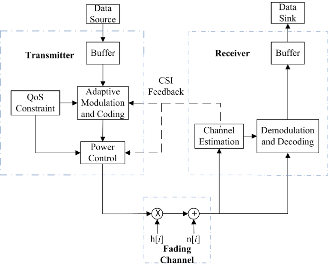
Figure 1: The system model

We consider a point-to-point communication system in which there is one source and one destination. The general system model is depicted in Fig.1, and is similar to the one studied in [17]. In this model, it is assumed that the source generates data sequences which are divided into frames of duration $T$. These data frames are initially stored in the buffer before they are transmitted over the wireless channel. The discrete-time channel input-output relation in the $i^{\text{th}}$ symbol duration is given by

$$y[i]=h[i]x[i]+n[i]\quad i=1,2,\ldots.$$ (1)

where $x[i]$ and $y[i]$ denote the complex-valued channel input and output, respectively. The channel input is subject to an average power constraint $\mathbb{E}\{|x[i]|^{2}\}\leq\bar{P}$ for all $i$, and we assume that the bandwidth available in the system is $B$. Above, $n[i]$ is a zero-mean, circularly symmetric, complex Gaussian random variable with variance $\mathbb{E}\{|n[i]|^{2}\}=N_{0}$. The additive Gaussian noise samples $\{n[i]\}$ are assumed to form an independent and identically distributed (i.i.d.) sequence. Finally, $h[i]$ denotes the channel fading coefficient, and $\{h[i]\}$ is a stationary and ergodic discrete-time process. We assume that perfect channel state information (CSI) is available at the receiver while the transmitter has either no or perfect CSI. The availability of CSI at the transmitter is facilitated through CSI feedback from the receiver. Note that if the transmitter knows the channel fading coefficients, it employs power and rate adaptation. Otherwise, the signals are sent with constant power.

Note that in the above system model, the average transmitted signal-to-noise ratio is ${\text{\footnotesize{SNR}}}=\bar{P}/(N_{0}B)$. We denote the magnitude-square of the fading coefficient by $z[i]=|h[i]|^{2}$, and its distribution function by $p_{z}(z)$. When there is only receiver CSI, instantaneous transmitted power is $P[i]=\bar{P}$ and the instantaneous received SNR is expressed as $\gamma[i]=\bar{P}z[i]/(N_{0}B)$. Moreover, the maximum instantaneous service rate $R[i]$ is

$$R[i]=B\log_{2}\Big{(}1+{\text{\footnotesize{SNR}}}z[i]\Big{)}\quad\text{bits/s}.$$ (2)

We note that although the transmitter does not know $z[i]$, recently developed rateless codes such as LT [24] and Raptor [25] codes enable the transmitter to adapt its rate to the channel realization and achieve $R[i]$ without requiring CSI at the transmitter side [26], [27].

When also the transmitter has CSI, the instantaneous service rate is

$$R[i]=B\log_{2}\Big{(}1+\mu_{\textrm{opt}}(\theta,z[i])z[i]\Big{)}\quad\text{bits/s}.$$ (3)

where $\mu_{\textrm{opt}}(\theta,z)$ is the optimal power-adaptation policy. The power policy that maximizes the effective capacity, which will be discussed in Section III-A, is determined in  [17]:

$$\mu_{\textrm{opt}}(\theta,z)=\begin{cases}\frac{1}{\alpha^{\frac{1}{\beta+1}}z^{\frac{\beta}{\beta+1}}}-\frac{1}{z}&z\geq\alpha\\ 0&z<\alpha\end{cases}$$ (4)

where $\beta=\frac{\theta TB}{\log_{e}{2}}$ is the normalized QoS exponent and $\alpha$ is the channel threshold chosen to satisfy the average power constraint:

$${\text{\footnotesize{SNR}}}=\mathbb{E}\{\mu_{\textrm{opt}}(\theta,z)\}=\mathbb{E}\bigg{\{}\bigg{[}\frac{1}{\alpha^{\frac{1}{\beta+1}}z^{\frac{\beta}{\beta+1}}}-\frac{1}{z}\bigg{]}\tau(\alpha)\bigg{\}}.$$ (5)

where $\tau(\alpha)=1\{z\geq\alpha\}=\left\{\begin{array}[]{ll}1&\text{if }z\geq\alpha\\ 0&\text{if }z<\alpha\end{array}\right.$ is the indicator function.

III Preliminaries

In this section, we briefly explain the notion of effective capacity and also describe the spectral efficiency-bit energy tradeoff. We refer the reader to [13] and [14] for more detailed exposition of the effective capacity.

III-A Effective Capacity

Satisfying quality of service (QoS) requirements is crucial for the successful deployment and operation of most communication networks. Hence, in the networking literature, how to handle and satisfy QoS constraints has been one of the key considerations for many years. In addressing this issue, the theory of effective bandwidth of a time-varying source has been developed to identify the minimum amount of transmission rate that is needed to satisfy the statistical QoS requirements (see e.g., [9], [10], [11], and [29]).

In wireless communications, the instantaneous channel capacity varies randomly depending on the channel conditions. Hence, in addition to the source, the transmission rates for reliable communication are also time-varying. The time-varying channel capacity can be incorporated into the theory of effective bandwidth by regarding the channel service process as a time-varying source with negative rate and using the source multiplexing rule ([29, Example 9.2.2]). Using a similar approach, Wu and Negi in [13] defined the effective capacity as a dual concept to effective bandwidth. The effective capacity provides the maximum constant arrival rate that a given time-varying service process can support while satisfying a QoS requirement specified by $\theta$. If we define $Q$ as the stationary queue length, then $\theta$ is the decay rate of the tail distribution of the queue length:

$$\lim_{q\to\infty}\frac{\log P(Q\geq q)}{q}=-\theta.$$ (6)

Therefore, for large $q_{\max}$, we have the following approximation for the buffer violation probability: $P(Q\geq q_{\max})\approx e^{-\theta q_{max}}$. Hence, while larger $\theta$ corresponds to more strict QoS constraints, smaller $\theta$ implies looser QoS guarantees. Similarly, if $D$ denotes the steady-state delay experienced in the buffer, then $P(D\geq d_{\max})\approx e^{-\theta\delta d_{\max}}$ for large $d_{\max}$, where $\delta$ is determined by the arrival and service processes [20]. The analysis and application of effect capacity in various settings has attracted much interest recently (see e.g., [14]–[21]).

Let $\{R[i],i=1,2,\ldots\}$ denote the discrete-time stationary and ergodic stochastic service process and $S[t]\triangleq\sum_{i=1}^{t}R[i]$ be the time-accumulated process. Assume that the Gärtner-Ellis limit of $S[t]$, expressed as [10]

$$\Lambda_{C}(\theta)=\lim_{t\rightarrow\infty}\frac{1}{t}\log_{e}{\mathbb{E}\{e^{\theta S[t]}\}}.$$ (7)

exists. Then, the effective capacity is given by  [13]

$$C_{E}({\text{\footnotesize{SNR}}},\theta)=-\frac{\Lambda_{C}(-\theta)}{\theta}=-\lim_{t\rightarrow\infty}\frac{1}{\theta t}\log_{e}{\mathbb{E}\{e^{-\theta S[t]}\}}.$$ (8)

If the fading process $\{h[i]\}$ is constant during the frame duration $T$ and changes independently from frame to frame, then the effective capacity simplifies to

$$C_{E}({\text{\footnotesize{SNR}}},\theta)=-\frac{1}{\theta T}\log_{e}\mathbb{E}\{e^{-\theta TR[i]}\}\quad\text{bits/s}.$$ (9)

This block-fading assumption is an approximation for practical wireless channels, and the independence assumption can be justified if, for instance, transmitted frames are interleaved before transmission, or time-division multiple access is employed and frame duration is proportional to the coherence time of the channel.

It can be easily shown that effective capacity specializes to the Shannon capacity and delay-limited capacity in the asymptotic regimes. As $\theta$ approaches to 0, constraints on queue length and queueing delay relax, and effective capacity converges to the Shannon ergodic capacity:

$$\lim_{\theta\to 0}C_{E}({\text{\footnotesize{SNR}}},\theta)=\left\{\begin{array}[]{ll}\mathbb{E}\{B\log_{2}(1+{\text{\footnotesize{SNR}}}z)\}&\text{CSI at the RX}\\ \mathbb{E}\left\{B\log_{2}\left(1+\mu_{\textrm{opt}}(\theta,z)z\right)\right\}&\text{CSI at the RX and TX}\end{array}\right.$$ (12)

where expectations are with respect to $z$. On the other hand, as $\theta\to\infty$, QoS constraints become more and more strict and effective capacity approaches the delay-limited capacity which as described before can be seen as a deterministic service guarantee:

$$\lim_{\theta\to\infty}C_{E}({\text{\footnotesize{SNR}}},\theta)=\left\{\begin{array}[]{ll}B\log_{2}(1+{\text{\footnotesize{SNR}}}z_{\min})&\text{CSI at the RX}\\ B\log_{2}\left(1+\sigma\right)&\text{CSI at the RX and TX}\end{array}\right.$$ (15)

where $\sigma=\frac{{\text{\footnotesize{SNR}}}}{\mathbb{E}\{1/z\}}$ and $z_{\min}$ is the minimum value of the random variable $z$, i.e., $z\geq z_{\min}\geq 0$ with probability 1. Note that in Rayleigh fading, $\sigma=0$ and $z_{\min}=0$, and hence the delay-limited capacities are zero in both cases and no deterministic guarantees can be provided.

III-B Spectral Efficiency vs. Bit Energy

In [2], Verdú has extensively studied the spectral efficiency–bit energy tradeoff in the wideband regime. In this work, the minimum bit energy required for reliable communication over a general class of multiple-input multiple-output channels is identified. In general, if the capacity is a concave function of SNR, then the minimum bit energy is achieved as ${\text{\footnotesize{SNR}}}\to 0$. Additionally, Verdú has defined the wideband slope, which is the slope of the spectral efficiency curve at zero spectral efficiency. While the minimum bit energy is a performance measure as ${\text{\footnotesize{SNR}}}\to 0$, wideband slope has emerged as a tool that enables us to analyze the energy efficiency at low but nonzero power levels and at large but finite bandwidths. In [2], the tradeoff between spectral efficiency and energy efficiency is analyzed considering the Shannon capacity. In this paper, we perform a similar analysis employing the effective capacity. Here, we denote the effective capacity normalized by bandwidth or equivalently the spectral efficiency in bits per second per Hertz by

$${\sf{C}}_{E}({\text{\footnotesize{SNR}}},\theta)=\frac{C_{E}({\text{\footnotesize{SNR}}},\theta)}{B}=-\frac{1}{\theta TB}\log_{e}\mathbb{E}\{e^{-\theta TR[i]}\}.$$ (16)

Hence, we characterize the spectral efficiency–bit energy tradeoff under QoS constraints. Note that effective capacity provides a characterization of the arrival process. However, since the average arrival rate is equal to the average departure rate when the queue is in steady-state [12], effective capacity can also be seen as a measure of the average rate of transmission. We first have the following preliminary result.

Lemma 1

The normalized effective capacity, ${\sf{C}}_{E}({\text{\footnotesize{SNR}}})$, given in (16) is a concave function of SNR.

Proof: It can be easily seen that $e^{-\theta TR[i]}$, where $R[i]=B\log_{2}(1+{\text{\footnotesize{SNR}}}z[i])$ or $R[i]=B\log_{2}(1+\mu_{\textrm{opt}}(\theta,z[i])z[i])$, is a log-convex function of SNR because $-R[i]$ is a convex function of SNR. Since log-convexity is preserved under sums, $g(x)=\int f(x,y)dy$ is log-convex in $x$ if $f(x,y)$ is log-convex in $x$ for each $y$ [30]. From this fact, we immediately conclude that $\mathbb{E}\{e^{-\theta TR[i]}\}$ is also a log-convex function of SNR. Hence, $\log_{e}\mathbb{E}\{e^{-\theta TR[i]}\}$ is convex and $-\log_{e}\mathbb{E}\{e^{-\theta TR[i]}\}$ is concave in SNR. $\square$

Then, it can be easily seen that $\frac{E_{b}}{N_{0}}_{\text{min}}$ under QoS constraints can be obtained from [2]

$$\frac{E_{b}}{N_{0}}_{\text{min}}=\lim_{{\text{\footnotesize{SNR}}}\rightarrow 0}\frac{{\text{\footnotesize{SNR}}}}{{\sf{C}}_{E}({\text{\footnotesize{SNR}}})}=\frac{1}{\dot{{\sf{C}}}_{E}(0)}.$$ (17)

At $\frac{E_{b}}{N_{0}}_{\text{min}}$, the slope $\mathcal{S}_{0}$ of the spectral efficiency versus $E_{b}/N_{0}$ (in dB) curve is defined as [2]

$$\mathcal{S}_{0}=\lim_{\frac{E_{b}}{N_{0}}\downarrow\frac{E_{b}}{N_{0}}_{\text{min}}}\frac{{\sf{C}}_{E}(\frac{E_{b}}{N_{0}})}{10\log_{10}\frac{E_{b}}{N_{0}}-10\log_{10}\frac{E_{b}}{N_{0}}_{\text{min}}}10\log_{10}2.$$ (18)

Considering the expression for normalized effective capacity, the wideband slope can be found from

$$\mathcal{S}_{0}=-\frac{2(\dot{{\sf{C}}}_{E}(0))^{2}}{\ddot{{\sf{C}}}_{E}(0)}\log_{e}{2}$$ (19)

where $\dot{{\sf{C}}}_{E}(0)$ and $\ddot{{\sf{C}}}_{E}(0)$ are the first and second derivatives, respectively, of the function ${\sf{C}}_{E}({\text{\footnotesize{SNR}}})$ in bits/s/Hz at zero SNR [2]. $\frac{E_{b}}{N_{0}}_{\text{min}}$ and $\mathcal{S}_{0}$ provide a linear approximation of the spectral efficiency curve at low spectral efficiencies, i.e.,

$${\sf{C}}_{E}\left(\frac{E_{b}}{N_{0}}\right)=\frac{\mathcal{S}_{0}}{10\log_{10}2}\left(\frac{E_{b}}{N_{0}}\bigg{|}_{dB}-\frac{E_{b}}{N_{0}}_{\text{min}}\bigg{|}_{dB}\right)+\epsilon$$ (20)

where $\frac{E_{b}}{N_{0}}\Big{|}_{dB}=10\log_{10}\frac{E_{b}}{N_{0}}$ and $\epsilon=o\left(\frac{E_{b}}{N_{0}}-\frac{E_{b}}{N_{0}}_{\text{min}}\right)$.

IV Energy Efficiency in the Low-Power Regime

As discussed in the previous section, the minimum bit energy is achieved as ${\text{\footnotesize{SNR}}}=\frac{\bar{P}}{N_{0}B}\to 0$, and hence energy efficiency improves if one operates in the low-power or high-bandwidth regime. From the Shannon capacity perspective, similar performances are achieved in these two regimes, which therefore can be seen as equivalent. However, as we shall see in this paper, considering the effective capacity leads to different results at low power and high bandwidth levels. In this section, we consider the low-power regime for fixed bandwidth, $B$, and study the spectral efficiency vs. bit energy tradeoff by finding the minimum bit energy and the wideband slope.

IV-A CSI at the Receiver Only

We initially consider the case in which only the receiver knows the channel conditions. Substituting (2) into (9), we obtain the spectral efficiency given $\theta$ as a function of SNR:

$${\sf{C}}_{E}({\text{\footnotesize{SNR}}})=-\frac{1}{\theta TB}\log_{e}{\mathbb{E}\{e^{-\theta TB\log_{2}(1+{\text{\footnotesize{SNR}}}z)}\}}=-\frac{1}{\theta TB}\log_{e}{\mathbb{E}\{(1+{\text{\footnotesize{SNR}}}z)^{-\beta}\}}$$ (21)

where again $\beta=\frac{\theta TB}{\log_{e}2}$. Note that since the analysis is performed for fixed $\theta$ throughout the paper, we henceforth express the effective capacity only as a function of SNR to simplify the expressions. The following result provides the minimum bit energy and the wideband slope.

Theorem 1

When only the receiver has perfect CSI, the minimum bit energy and wideband slope are

$$\frac{E_{b}}{N_{0}}_{\text{min}}=\frac{\log_{e}{2}}{\mathbb{E}\{z\}}\text{ and }\mathcal{S}_{0}=\frac{2}{(\beta+1)\frac{\mathbb{E}\{z^{2}\}}{\big{(}\mathbb{E}\{z\}\big{)}^{2}}-\beta}.$$ (22)

Proof: The first and second derivative of ${\sf{C}}_{E}({\text{\footnotesize{SNR}}})$ with respect to SNR are given by

$$\dot{{\sf{C}}}_{E}({\text{\footnotesize{SNR}}})=\frac{1}{\log_{e}{2}}\frac{\mathbb{E}\{(1+{\text{\footnotesize{SNR}}}z)^{-(\beta+1)}z\}}{\mathbb{E}\{(1+{\text{\footnotesize{SNR}}}z)^{-\beta}\}}\quad\text{and,}$$ (23)

$$\ddot{{\sf{C}}}_{E}({\text{\footnotesize{SNR}}})=\frac{\beta}{\log_{e}{2}}\bigg{(}\frac{\mathbb{E}\{(1+{\text{\footnotesize{SNR}}}z)^{-(\beta+1)}z\}}{\mathbb{E}\{(1+{\text{\footnotesize{SNR}}}z)^{-\beta}\}}\bigg{)}^{2}-\frac{\beta+1}{\log_{e}{2}}\frac{\mathbb{E}\{(1+{\text{\footnotesize{SNR}}}z)^{-(\beta+2)}z^{2}\}}{\mathbb{E}\{(1+{\text{\footnotesize{SNR}}}z)^{-\beta}\}},$$ (24)

respectively, which result in the following expressions when ${\text{\footnotesize{SNR}}}=0$:

$$\dot{{\sf{C}}}_{E}(0)=\frac{\mathbb{E}\{z\}}{\log_{e}{2}}\quad\text{and}\quad\ddot{{\sf{C}}}_{E}(0)=-\frac{1}{\log_{e}{2}}\Big{(}(\beta+1)\mathbb{E}\{z^{2}\}-\beta\big{(}\mathbb{E}\{z\}\big{)}^{2}\Big{)}.$$ (25)

Substituting the expressions in (25) into (17) and (19) provides the desired result. $\square$

From the above result, we immediately see that $\frac{E_{b}}{N_{0}}_{\min}$ does not depend on $\theta$ and the minimum received bit energy is

$$\frac{E_{b}^{r}}{N_{0}}_{\text{min}}=\frac{E_{b}}{N_{0}}_{\text{min}}\mathbb{E}\{z\}=\log_{e}2=-1.59\text{ dB}.$$ (26)

Note that if the Shannon capacity is used in the analysis, i.e., if $\theta=0$ and hence $\beta=0$, $\frac{E_{b}^{r}}{N_{0}}_{\text{min}}=-1.59$ dB and $\mathcal{S}_{0}=2/(\mathbb{E}\{z^{2}\}/\mathbb{E}^{2}\{z\})$. Therefore, we conclude from Theorem 1 that as the average power $\bar{P}$ decreases, energy efficiency approaches the performance achieved by a system that does not have QoS limitations. However, we note that wideband slope is smaller if $\theta>0$. Hence, the presence of QoS constraints decreases the spectral efficiency or equivalently increases the energy requirements for fixed spectral efficiency values at low but nonzero SNR levels.

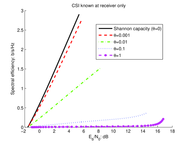
Figure 2: Spectral efficiency vs. $E_{b}/N_{0}$ in the Rayleigh fading channel with fixed $B$; CSI known at the receiver only.

Fig. 2 plots the spectral efficiency as a function of the bit energy for different values of $\theta$ in the Rayleigh fading channel with $\mathbb{E}\{|h|^{2}\}=\mathbb{E}\{z\}=1$. Note that the curve for $\theta=0$ corresponds to the Shannon capacity. Throughout the paper, we set the frame duration to $T=2$ms in the numerical results. For the fixed bandwidth case, we have assumed $B=10^{5}$ Hz. In Fig. 2, we observe that all curves approach $\frac{E_{b}}{N_{0}}_{\text{min}}=-1.59$ dB as predicted. On the other hand, we note that the wideband slope decreases as $\theta$ increases. Therefore, at low but nonzero spectral efficiencies, more energy is required as the QoS constraints become more stringent. Considering the linear approximation in (20), we can easily show for fixed spectral efficiency ${\sf{C}}\left(\frac{E_{b}}{N_{0}}\right)$ for which the linear approximation is accurate that the increase in the bit energy in dB, when the QoS exponent increases from $\theta_{1}$ to $\theta_{2}$, is

$$\frac{E_{b}}{N_{0}}\bigg{|}_{dB,\theta_{2}}-\frac{E_{b}}{N_{0}}\bigg{|}_{dB,\theta_{1}}=\left(\frac{1}{\mathcal{S}_{0,\theta_{2}}}-\frac{1}{\mathcal{S}_{0,\theta_{1}}}\right){\sf{C}}\left(\frac{E_{b}}{N_{0}}\right)10\log_{10}2.$$ (27)

IV-B CSI at both the Transmitter and Receiver

We now consider the case in which both the transmitter and receiver have perfect CSI. Substituting (3) into (9), we have

$${\sf{C}}_{E}({\text{\footnotesize{SNR}}})=-\frac{1}{\theta TB}\log_{e}\mathbb{E}\Big{\{}e^{-\theta TB\log_{2}\big{(}1+\mu_{\textrm{opt}}(\theta,z)z\big{)}}\Big{\}}=-\frac{1}{\theta TB}\log_{e}\Big{(}F(\alpha)+\mathbb{E}\Big{\{}\left(\frac{z}{\alpha}\right)^{-\frac{\beta}{\beta+1}}\tau(\alpha)\Big{\}}\Big{)}$$ (28)

where $F(\alpha)=\mathbb{E}\{1\{z<\alpha\}\}$. For this case, following an approach similar to that in [22], we obtain the following result.

Theorem 2

When both the transmitter and receiver have perfect CSI, the minimum bit energy with optimal power control and rate adaptation becomes

$$\frac{E_{b}}{N_{0}}_{\text{min}}=\frac{\log_{e}2}{z_{\max}}$$ (29)

where $z_{\max}$ is the essential supremum of the random variable $z$, i.e., $z\leq z_{\max}$ with probability 1.

Proof: We assume that $z_{\text{max}}$ is the maximum value that the random variable $z$ can take, i.e., $P(z\leq z_{\text{max}})=1$. From (5), we can see that as SNR vanishes, $\alpha$ increases to $z_{\max}$, because otherwise while SNR approaches zero, the right most side of (5) does not. Then, we can suppose for small enough SNR that

$$\alpha=z_{\text{max}}-\eta$$ (30)

where $\eta\rightarrow 0$ as ${\text{\footnotesize{SNR}}}\rightarrow 0$. Substituting (30) into (5) and (28), we get

$$\frac{E_{b}}{N_{0}}_{\text{min}}=\lim_{{\text{\footnotesize{SNR}}}\rightarrow 0}\frac{{\text{\footnotesize{SNR}}}}{{\sf{C}}({\text{\footnotesize{SNR}}})} =\lim_{\eta\rightarrow 0}\frac{\mathbb{E}\bigg{\{}\Big{[}\frac{1}{(z_{\text{max}}-\eta)^{\frac{1}{\beta+1}}z^{\frac{\beta}{\beta+1}}}-\frac{1}{z}\Big{]}\tau(z_{\text{max}}-\eta)\bigg{\}}}{-\frac{1}{\theta TB}\log_{e}\Big{(}F(z_{\text{max}}-\eta)+\mathbb{E}\Big{\{}\big{(}\frac{z}{z_{\text{max}}-\eta}\big{)}^{-\frac{\beta}{\beta+1}}\tau(z_{\text{max}}-\eta)\Big{\}}\Big{)}}$$ (31)

$$=\lim_{\eta\rightarrow 0}\frac{\int_{z_{\text{max}}-\eta}^{z_{\text{max}}}\bigg{(}\frac{1}{(z_{\text{max}}-\eta)^{\frac{1}{\beta+1}}z^{\frac{\beta}{\beta+1}}}-\frac{1}{z}\bigg{)}p_{z}(z)dz}{-\frac{1}{\theta TB}\log_{e}\bigg{(}\int_{0}^{z_{\text{max}}-\eta}p_{z}(z)dz+\int_{z_{\text{max}}-\eta}^{z_{\text{max}}}\big{(}\frac{z}{z_{\text{max}}-\eta}\big{)}^{-\frac{\beta}{\beta+1}}p_{z}(z)dz\bigg{)}}$$ (32)

$$=\lim_{\eta\rightarrow 0}\frac{\frac{1}{\beta+1}(z_{\text{max}}-\eta)^{-\frac{\beta+2}{\beta+1}}\int_{z_{\text{max}}-\eta}^{z_{\text{max}}}\frac{p_{z}(z)}{z^{\frac{\beta}{\beta+1}}}dz}{-\frac{1}{\beta\log_{e}2}\frac{-\frac{\beta}{\beta+1}(z_{\text{max}}-\eta)^{-\frac{1}{\beta+1}}\int_{z_{\text{max}}-\eta}^{z_{\text{max}}}\frac{p_{z}(z)}{z^{\frac{\beta}{\beta+1}}}dz}{\int_{0}^{z_{\text{max}}-\eta}p_{z}(z)dz+\int_{z_{\text{max}}-\eta}^{z_{\text{max}}}\big{(}\frac{z}{z_{\text{max}}-\eta}\big{)}^{-\frac{\beta}{\beta+1}}p_{z}(z)dz}}$$ (33)

$$=\lim_{\eta\rightarrow 0}\frac{\Big{(}\int_{0}^{z_{\text{max}}-\eta}p_{z}(z)dz+\int_{z_{\text{max}}-\eta}^{z_{\text{max}}}\big{(}\frac{z}{z_{\text{max}}-\eta}\big{)}^{-\frac{\beta}{\beta+1}}p_{z}(z)dz\Big{)}\log_{e}2}{z_{\text{max}}-\eta}=\frac{\log_{e}2}{z_{\text{max}}}$$ (34)

where $p_{z}$ is the distribution of channel gain $z$. (32) is obtained by expressing the expectations in (31) as integrals. (33) follows by using the L’Hospital’s Rule and applying Leibniz Integral Rule. The first term in (34) is obtained after straightforward algebraic simplifications and the result follows immediately. $\square$

Note that for distributions with unbounded support, we have $z_{\max}=\infty$ and hence $\frac{E_{b}}{N_{0}}_{\text{min}}=0=-\infty$ dB. In this case, it is easy to see that the wideband slope is $S_{0}=0$.

Example 1

Specifically, for the Rayleigh fading channel, as in  [23], it can be shown that
$\lim_{{\text{\footnotesize{SNR}}}\rightarrow 0}{\frac{{\sf{C}}_{E}({\text{\footnotesize{SNR}}})}{{\text{\footnotesize{SNR}}}\log_{e}(\frac{1}{{\text{\footnotesize{SNR}}}})\log_{e}{2}}}=1.$ Then, spectral efficiency can be written as ${\sf{C}}_{E}({\text{\footnotesize{SNR}}})\approx{\text{\footnotesize{SNR}}}\log_{e}(\frac{1}{{\text{\footnotesize{SNR}}}})\log_{e}{2}$, so $\frac{E_{b}}{N_{0}}_{\textrm{min}}=\lim_{{\text{\footnotesize{SNR}}}\rightarrow 0}\frac{{\text{\footnotesize{SNR}}}}{{\sf{C}}_{E}({\text{\footnotesize{SNR}}})}=\lim_{{\text{\footnotesize{SNR}}}\rightarrow 0}\frac{1}{\log_{e}(\frac{1}{{\text{\footnotesize{SNR}}}})\log_{e}{2}}=0$ which also verifies the above result.

Remark: We note that as in the case in which there is CSI at the receiver, the minimum bit energy achieved under QoS constraints is the same as that achieved by the Shannon capacity [22]. Hence, the energy efficiency again approaches the performance of an unconstrained system as power diminishes. Searching for an intuitive explanation of this observation, we note that arrival rates that can be supported vanishes with decreasing power levels. As a result, the impact of buffer occupancy constraints on the performance lessens. Note that in contrast, increasing the bandwidth increases the arrival rates supported by the system. Therefore, limitations on the buffer occupancy will have significant impact upon the energy efficiency in the wideband regime as will be discussed in Section V.

Fig. 3 plots the spectral efficiency vs. bit energy for different values of $\theta$ in the Rayleigh fading channel with $\mathbb{E}\{z\}=1$. In all cases, we observe that the bit energy goes to $-\infty$ as the spectral efficiency decreases. We also note that at small but nonzero spectral efficiencies, the required energy is higher as $\theta$ increases.

V Energy Efficiency in the Wideband Regime

In this section, we study the performance at high bandwidths while the average power $\bar{P}$ is kept fixed. We investigate the impact of $\theta$ on $\frac{E_{b}}{N_{0}}_{\text{min}}$ and the wideband slope $\mathcal{S}_{0}$ in this wideband regime. Note that as the bandwidth increases, the average signal-to-noise ratio ${\text{\footnotesize{SNR}}}=\bar{P}/(N_{0}B)$ and the spectral efficiency decreases.

V-A CSI at the Receiver Only

We define $\zeta=\frac{1}{B}$ and express the spectral efficiency (21) as a function of $\zeta$:

$${\sf{C}}_{E}(\zeta)=-\frac{\zeta}{\theta T}\log_{e}{\mathbb{E}\{e^{-\frac{\theta T}{\zeta}\log_{2}(1+\frac{\bar{P}\zeta}{N_{0}}z)}\}}.$$ (35)

The bit energy is again defined as

$$\frac{E_{b}}{N_{0}}=\frac{{\text{\footnotesize{SNR}}}}{{\sf{C}}_{E}({\text{\footnotesize{SNR}}})}=\frac{\frac{\bar{P}\zeta}{N_{0}}}{{\sf{C}}_{E}(\zeta)}=\frac{\frac{\bar{P}}{N_{0}}}{{\sf{C}}_{E}(\zeta)/\zeta}.$$ (36)

It can be readily verified that ${\sf{C}}_{E}(\zeta)/\zeta$ monotonically increases as $\zeta\to 0$ (or equivalently as $B\to\infty$) (see Appendix A). Therefore

$$\frac{E_{b}}{N_{0}}_{\text{min}}=\lim_{\zeta\rightarrow 0}\frac{\bar{P}\zeta/N_{0}}{{\sf{C}}_{E}(\zeta)}=\frac{\bar{P}/N_{0}}{\dot{{\sf{C}}}_{E}(0)}$$ (37)

where $\dot{{\sf{C}}}_{E}(0)$ is the first derivative of the spectral efficiency with respect to $\zeta$ at $\zeta=0$. The wideband slope $\mathcal{S}_{0}$ can be obtained from the formula (19) by using the first and second derivatives of the spectral efficiency ${\sf{C}}_{E}(\zeta)$ with respect to $\zeta$.

Theorem 3

When only the receiver has CSI, the minimum bit energy and wideband slope, respectively, in the wideband regime are given by

$$\frac{E_{b}}{N_{0}}_{\text{min}}=\frac{-\frac{\theta T\bar{P}}{N_{0}}}{\log_{e}\mathbb{E}\{e^{-\frac{\theta T\bar{P}}{N_{0}\log_{2}}z}\}},\quad\text{and}$$ (38)

$$\mathcal{S}_{0}=2\Big{(}\frac{N_{0}\log_{e}2}{\theta T\bar{P}}\Big{)}^{2}\frac{\mathbb{E}\{e^{-\frac{\theta T\bar{P}}{N_{0}\log_{e}2}z}\}\Big{(}\log_{e}\mathbb{E}\{e^{-\frac{\theta T\bar{P}}{N_{0}\log_{e}2}z}\}\Big{)}^{2}}{\mathbb{E}\{e^{-\frac{\theta T\bar{P}}{N_{0}\log_{e}2}z}z^{2}\}}.$$ (39)

Proof: The first and second derivative of ${\sf{C}}_{E}(\zeta)$ are given by

$$\dot{{\sf{C}}}_{E}(\zeta)=-\frac{1}{\theta T}\log_{e}\mathbb{E}\{e^{-\frac{\theta T}{\zeta}\log_{2}(1+\frac{\bar{P}\zeta z}{N_{0}})}\}-\frac{\mathbb{E}\bigg{\{}e^{-\frac{\theta T}{\zeta}\log_{2}(1+\frac{\bar{P}\zeta z}{N_{0}})}\Bigl{[}\frac{\log_{2}(1+\frac{\bar{P}\zeta z}{N_{0}})}{\zeta}-\frac{\frac{\bar{P}z}{N_{0}\log_{e}{2}}}{1+\frac{\bar{P}\zeta z}{N_{0}}}\Bigr{]}\bigg{\}}}{\mathbb{E}\{e^{-\frac{\theta T}{\zeta}\log_{2}(1+\frac{\bar{P}\zeta z}{N_{0}})}\}},$$ (40)

$$\begin{split}\ddot{{\sf{C}}}_{E}(\zeta)&=\frac{\theta T}{\zeta}\left(\frac{\mathbb{E}\bigg{\{}e^{-\frac{\theta T}{\zeta}\log_{2}(1+\frac{\bar{P}\zeta z}{N_{0}})}\Bigl{[}\frac{\log_{2}(1+\frac{\bar{P}\zeta z}{N_{0}})}{\zeta}-\frac{\frac{\bar{P}z}{N_{0}\log_{e}{2}}}{1+\frac{\bar{P}\zeta z}{N_{0}}}\Bigr{]}\bigg{\}}}{\mathbb{E}\{e^{-\frac{\theta T}{\zeta}\log_{2}(1+\frac{\bar{P}\zeta z}{N_{0}})}\}}\right)^{2}\\ &\phantom{{=}\frac{\theta T}{\zeta}}-\frac{\mathbb{E}\bigg{\{}e^{-\frac{\theta T}{\zeta}\log_{2}(1+\frac{\bar{P}\zeta z}{N_{0}})}\biggl{[}\frac{\theta T}{\zeta}\Bigl{(}\frac{\log_{2}(1+\frac{\bar{P}\zeta z}{N_{0}})}{\zeta}-\frac{\frac{\bar{P}z}{N_{0}\log_{e}{2}}}{1+\frac{\bar{P}\zeta z}{N_{0}}}\Bigr{)}^{2}+\log_{e}{2}\Big{(}\frac{\frac{\bar{P}z}{N_{0}\log_{e}{2}}}{1+\frac{\bar{P}\zeta z}{N_{0}}}\Big{)}^{2}\biggr{]}\bigg{\}}}{\mathbb{E}\{e^{-\frac{\theta T}{\zeta}\log_{2}(1+\frac{\bar{P}\zeta z}{N_{0}})}\}}\end{split}.$$ (41)

First, we define the function $f(\zeta)=\frac{\log_{2}(1+\frac{\bar{P}\zeta z}{N_{0}})}{\zeta^{2}}-\frac{\frac{\bar{P}z}{N_{0}\zeta\log_{e}{2}}}{1+\frac{\bar{P}\zeta z}{N_{0}}}.$ Then, we can show that

$$\begin{split}\lim_{\zeta\rightarrow 0}{f(\zeta)}=\lim_{\zeta\rightarrow 0}{\frac{\frac{\log_{2}(1+\frac{\bar{P}\zeta z}{N_{0}})}{\zeta}-\frac{\frac{\bar{P}z}{N_{0}\log_{e}{2}}}{1+\frac{\bar{P}\zeta z}{N_{0}}}}{\zeta}}&=\lim_{\zeta\rightarrow 0}\biggl{(}-\frac{\log_{2}(1+\frac{\bar{P}\zeta z}{N_{0}})}{\zeta^{2}}+\frac{\frac{\bar{P}z}{N_{0}\log_{e}{2}}}{1+\frac{\bar{P}\zeta z}{N_{0}}}+\Bigl{(}\frac{\frac{\bar{P}z}{N_{0}\log_{e}{2}}}{1+\frac{\bar{P}\zeta z}{N_{0}}}\Bigr{)}^{2}\log_{e}{2}\biggr{)}\\ &=-\lim_{\zeta\rightarrow 0}{f(\zeta)}+\frac{1}{\log_{e}{2}}\left(\frac{\bar{P}z}{N_{0}}\right)^{2}\\ \end{split}$$

which yields

$$\lim_{\zeta\rightarrow 0}{f(\zeta)}=\frac{1}{2\log_{e}{2}}\left(\frac{\bar{P}z}{N_{0}}\right)^{2}$$ (42)

Using (42), we can easily find from (40) that

$$\lim_{\zeta\rightarrow 0}{\dot{{\sf{C}}}_{E}(\zeta)}=-\frac{1}{\theta T}\log_{e}\mathbb{E}\left\{e^{-\frac{\theta T\bar{P}}{N_{0}\log_{e}{2}}z}\right\}$$ (43)

from which (38) follows immediately. Moreover, from (41), we can derive

$$\lim_{\zeta\rightarrow 0}{\ddot{{\sf{C}}}_{E}(\zeta)}=-\frac{1}{\log_{e}2}\Big{(}\frac{\bar{P}}{N_{0}}\Big{)}^{2}\frac{\mathbb{E}\{e^{-\frac{\theta T\bar{P}}{N_{0}\log_{e}2}z}z^{2}\}}{\mathbb{E}\{e^{-\frac{\theta T\bar{P}}{N_{0}\log_{e}2}z}\}}.$$ (44)

Evaluating (19) with (43) and (44) provides (39). $\square$

It is interesting to note that unlike the low-power regime results, we now have

$$\frac{E_{b}}{N_{0}}_{\text{min}}=\frac{-\frac{\theta T\bar{P}}{N_{0}}}{\log_{e}\mathbb{E}\{e^{-\frac{\theta T\bar{P}}{N_{0}\log_{e}2}z}\}}\geq\frac{-\frac{\theta T\bar{P}}{N_{0}}}{\mathbb{E}\{\log_{e}e^{-\frac{\theta T\bar{P}}{N_{0}\log_{e}2}z}\}}=\frac{\log_{e}2}{\mathbb{E}\{z\}}$$

where Jensen’s inequality is used. Therefore, we will be operating above $-1.59$ dB unless there are no QoS constraints and hence $\theta=0$. For the Rayleigh channel, we can specialize (38) and (39) to obtain

$$\frac{E_{b}}{N_{0}}_{\textrm{min}}=\frac{\frac{\theta T\bar{P}}{N_{0}}}{\log_{e}(1+\frac{\theta T\bar{P}}{N_{0}\log_{e}2})}\quad\text{and}\quad\mathcal{S}_{0}=\bigg{(}\frac{N_{0}\log_{e}2}{\theta T\bar{P}}\log_{e}(1+\frac{\theta T\bar{P}}{N_{0}\log_{e}2})+\log_{e}(1+\frac{\theta T\bar{P}}{N_{0}\log_{e}{2}})\bigg{)}^{2}.$$ (45)

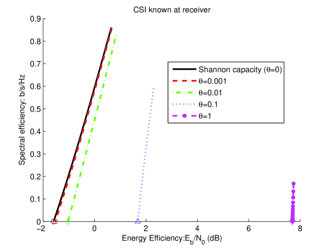
Figure 4: Spectral efficiency vs. $E_{b}/N_{0}$ in the Rayleigh fading channel with fixed $\bar{P}$; CSI known at the receiver only.

It can be easily seen that in the Rayleigh channel, the minimum bit energy monotonically increases with increasing $\theta$. Fig. 4 plots the spectral efficiency curves as a function of bit energy in the Rayleigh channel. In all the curves, we set $\bar{P}/N_{0}=10^{4}$. We immediately observe that more stringent QoS constraints and hence higher values of $\theta$ lead to higher minimum bit energy values and also higher energy requirements at other nonzero spectral efficiencies. The wideband slope values are found to be equal to $\mathcal{S}_{0}=\{1.0288,1.2817,3.3401,12.3484\}$ for $\theta=\{0.001,0.01,0.1,1\}$, respectively.

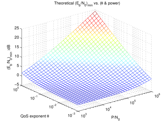
Figure 5: $\frac{E_{b}}{N_{0}}_{\textrm{min}}$ vs. $\theta$ and $\bar{P}/N_{0}$ in the Rayleigh fading channel; CSI known at the receiver only.

We finally note that $\frac{E_{b}}{N_{0}}_{\text{min}}$ and $\mathcal{S}_{0}$ now depend on $\theta$ and $\frac{\bar{P}}{N_{0}}$. Fig. 5 plots $\frac{E_{b}}{N_{0}}_{\text{min}}$ as a function of these two parameters. Probing into the inherent relationships among these parameters can give us some interesting results, which are helpful in designing wireless networks. For instance, for some $\bar{P}/N_{0}$ required to achieve some specific transmission rate, we can find the most stringent QoS guarantee possible while attaining a certain efficiency in the usage of energy, or if a QoS requirement $\theta$ is specified, we can find the minimum power $\bar{P}$ to achieve a specific bit energy.

V-B CSI at both the Transmitter and Receiver

To analyze $\frac{E_{b}}{N_{0}}_{\text{min}}$ in this case, we initially obtain the following result and identify the limiting value of the threshold $\alpha$ as the bandwidth increases to infinity.

Theorem 4

In wideband regime, the threshold $\alpha$ in the optimal power adaptation scheme (4) satisfies

$$\lim_{\zeta\rightarrow 0}\alpha(\zeta)=\alpha^{\ast}$$ (46)

where $\alpha^{\ast}$ is the solution to

$$\mathbb{E}\left\{\left[\log_{e}\left(\frac{z}{\alpha^{\ast}}\right)\frac{1}{z}\right]\tau(\alpha^{\ast})\right\}=\frac{\theta T\bar{P}}{N_{0}\log_{e}{2}}.$$ (47)

Moreover, for $\theta>0$, ${\alpha^{\ast}}<\infty$.

Proof: Recall from (5) that the optimal power adaptation rule should satisfy the average power constraint:

$${\text{\footnotesize{SNR}}}=\frac{\bar{P}\zeta}{N_{0}} =\mathbb{E}\bigg{\{}\Big{(}\frac{1}{\alpha^{\frac{1}{\beta+1}}z^{\frac{\beta}{\beta+1}}}-\frac{1}{z}\Big{)}\tau(\alpha)\bigg{\}}=\mathbb{E}\bigg{\{}\bigg{[}\bigg{(}\Big{(}\frac{z}{\alpha}\Big{)}^{\frac{1}{\beta+1}}-1\bigg{)}\frac{1}{z}\bigg{]}\tau(\alpha)\bigg{\}}$$ (48)

where $\beta=\frac{\theta TB}{\log_{e}2}=\frac{\theta T}{\zeta\log_{e}2}$. For the case in which $\theta=0$, if we let $\zeta\to 0$, we obtain from (48) that

$$0=\mathbb{E}\left\{\left[\left(\frac{z}{{\alpha^{\ast}}}-1\right)\frac{1}{z}\right]\tau({\alpha^{\ast}})\right\}$$ (49)

where ${\alpha^{\ast}}=\lim_{\zeta\to 0}\alpha(\zeta)$. Using the fact that $\log_{e}x\leq x-1$ for $x\geq 1$, we have $\log_{e}\left(\frac{z}{{\alpha^{\ast}}}\right)\leq\frac{z}{{\alpha^{\ast}}}-1$ for $z\geq{\alpha^{\ast}}$ which implies that

$$0\leq\mathbb{E}\left\{\left[\log_{e}\left(\frac{z}{\alpha^{\ast}}\right)\frac{1}{z}\right]\tau(\alpha^{\ast})\right\}\leq\mathbb{E}\left\{\left[\left(\frac{z}{{\alpha^{\ast}}}-1\right)\frac{1}{z}\right]\tau({\alpha^{\ast}})\right\}=0\implies\mathbb{E}\left\{\left[\log_{e}\left(\frac{z}{\alpha^{\ast}}\right)\frac{1}{z}\right]\tau(\alpha^{\ast})\right\}=0$$

proving (47) for the case of $\theta=0$.

In the following, we assume $\theta>0$. We first define $g(\zeta)=\left(\frac{z}{\alpha}\right)^{\frac{1}{\beta+1}}=\left(\frac{z}{\alpha}\right)^{\frac{\zeta\log_{e}2}{\zeta\log_{e}2+\theta T}}$ and take the logarithm of both sides to obtain

$$\log_{e}g(\zeta)=\frac{\zeta\log_{e}2}{\zeta\log_{e}2+\theta T}\log_{e}\frac{z}{\alpha}.$$ (50)

Differentiation over both sides leads to

$$\frac{\dot{g}(\zeta)}{g(\zeta)}=\frac{\theta T\log_{e}2}{(\zeta\log_{e}2+\theta T)^{2}}\log_{e}\frac{z}{\alpha}-\frac{\zeta\log_{e}2}{\zeta\log_{e}2+\theta T}\frac{\dot{\alpha}}{\alpha}$$ (51)

where $\dot{g}$ and $\dot{\alpha}$ denote the first derivatives $g$ and $\alpha$, respectively, with respect to $\zeta$. Noting that $g(0)=1$, we can see from (51) that as $\zeta\to 0$, we have

$$\dot{g}(0)=\frac{\log_{e}2}{\theta T}\log_{e}\frac{z}{{\alpha^{\ast}}}$$ (52)

where ${\alpha^{\ast}}=\lim_{\zeta\rightarrow 0}\alpha(\zeta)$. For small values of $\zeta$, the function $g$ admits the following Taylor series:

$$g(\zeta)=\left(\frac{z}{\alpha}\right)^{\frac{1}{\beta+1}}=g(0)+\dot{g}(0)\zeta+o(\zeta)=1+\dot{g}(0)\zeta+o(\zeta).$$ (53)

Therefore, we have

$$\Big{(}\frac{z}{\alpha}\Big{)}^{\frac{1}{\beta+1}}-1=\frac{\log_{e}2}{\theta T}\log_{e}\left(\frac{z}{{\alpha^{\ast}}}\right)\zeta+o(\zeta).$$ (54)

Then, from (48), we can write

$${\text{\footnotesize{SNR}}}=\mathbb{E}\left\{\left[\left(\frac{\log_{e}2}{\theta T}\log_{e}\left(\frac{z}{\alpha}\right)\zeta+o(\zeta)\right)\,\frac{1}{z}\right]\tau(\alpha)\right\}.$$ (55)

If we divide both sides of (55) by ${\text{\footnotesize{SNR}}}=\frac{\bar{P}\zeta}{N_{0}}$ and let $\zeta\to 0$, we obtain

$$\lim_{\zeta\rightarrow 0}\frac{{\text{\footnotesize{SNR}}}}{{\text{\footnotesize{SNR}}}}=\lim_{\zeta\rightarrow 0}\frac{{\text{\footnotesize{SNR}}}}{\frac{\bar{P}\zeta}{N_{0}}}=1=\frac{N_{0}\log_{e}2}{\theta T\bar{P}}\mathbb{E}\left\{\left[\log_{e}\left(\frac{z}{{\alpha^{\ast}}}\right)\frac{1}{z}\right]\tau({\alpha^{\ast}})\right\}$$ (56)

from which we conclude that $\mathbb{E}\left\{\left[\log_{e}\left(\frac{z}{\alpha^{\ast}}\right)\frac{1}{z}\right]\tau(\alpha^{\ast})\right\}=\frac{\theta T\bar{P}}{N_{0}\log_{e}{2}}$, proving (47) for $\theta>0$.

Using the fact that $\log_{e}\left(\frac{z}{\alpha}\right)<\frac{z}{\alpha}$ for $z\geq 0$, we can write

$$0\leq\mathbb{E}\left\{\left[\log_{e}\left(\frac{z}{\alpha}\right)\frac{1}{z}\right]\tau(\alpha)\right\}\leq\mathbb{E}\bigg{\{}\frac{1}{\alpha}\tau(\alpha)\bigg{\}}\leq\frac{1}{\alpha}.$$ (57)

Assume now that $\lim_{\zeta\to 0}\alpha(\zeta)={\alpha^{\ast}}=\infty$. Then, the rightmost side of (57) becomes zero in the limit as $\zeta\to 0$ which implies that $\mathbb{E}\left\{\left[\log_{e}\left(\frac{z}{{\alpha^{\ast}}}\right)\frac{1}{z}\right]\tau({\alpha^{\ast}})\right\}=0$. From (47), this is clearly not possible for $\theta>0$. Hence, we have proved that ${\alpha^{\ast}}<\infty$ when $\theta>0$. $\square$

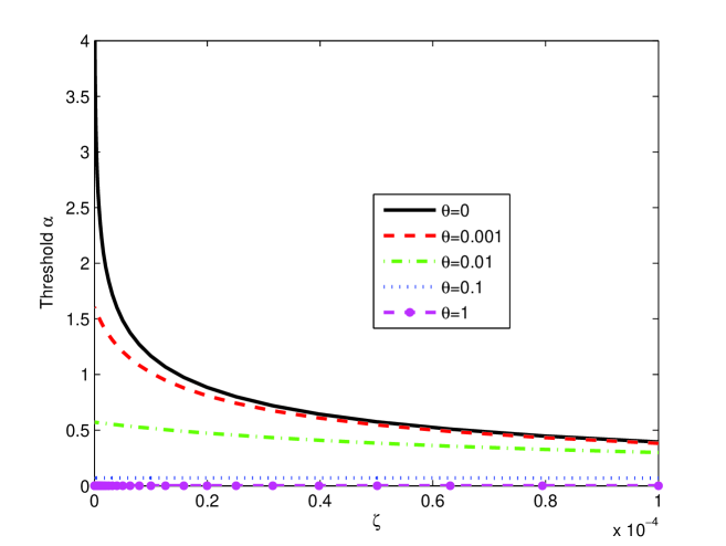
Figure 6: Threshold of channel gain $\alpha$ vs. $\zeta$ in the Rayleigh fading channel; CSI known at the transmitter and receiver.

Remark: As noted before, wideband and low-power regimes are equivalent when $\theta=0$. Hence, as in the proof of Theorem 2, we can easily see in the wideband regime that the threshold $\alpha$ approaches the maximum fading value $z_{\max}$ as $\zeta\to 0$ when $\theta=0$. Hence, for fading distributions with unbounded support, $\alpha\to\infty$ with vanishing $\zeta$. The threshold being very large means that the transmitter waits sufficiently long until the fading assumes very large values and becomes favorable. That is how arbitrarily small bit energy values can be attained. However, in the presence of QoS constraints, arbitrarily long waiting times will not be permitted. As a result, $\alpha$ approaches a finite value (i.e., ${\alpha^{\ast}}<\infty$) as $\zeta\to 0$ when $\theta>0$. Moreover, from (47), we can immediately note that as $\theta$ increases, ${\alpha^{\ast}}$ has to decrease. This fact can also be observed in Fig. 6 in which $\alpha$ vs. $\zeta$ is plotted in the Rayleigh fading channel. Consequently, arbitrarily small bit energy values will no longer be possible when $\theta>0$ as will be shown in Theorem 5.

The spectral efficiency with optimal power adaptation is now given by

$${\sf{C}}_{E}(\zeta)=-\frac{\zeta}{\theta T}\log_{e}\Big{(}F(\alpha)+\mathbb{E}\Big{\{}\Big{(}\frac{z}{\alpha}\Big{)}^{-\frac{\theta T}{\theta T+\zeta\log_{e}{2}}}\tau(\alpha)\Big{\}}\Big{)}$$ (58)

where again $F(\alpha)=\mathbb{E}\{1\{z<\alpha\}\}$ and $\tau(\alpha)=1\{\tau\geq\alpha\}$.

Theorem 5

When both the receiver and transmitter have CSI, the minimum bit energy and wideband slope in the wideband regime are given by

$$\frac{E_{b}}{N_{0}}_{\min}=-\frac{\theta T\bar{P}}{N_{0}\log_{e}\xi}\text{ and }\mathcal{S}_{0}=\frac{\xi(\log_{e}\xi)^{2}\log_{e}2}{\theta T(\frac{\bar{P}{\alpha^{\ast}}}{N_{0}}+\dot{\alpha}(0)\mathbb{E}\{\frac{1}{z}\tau({\alpha^{\ast}})\})}$$ (59)

where $\xi=F(\alpha^{\ast})+\mathbb{E}\{\frac{\alpha^{\ast}}{z}\tau(\alpha^{\ast})\}$, and $\dot{\alpha}(0)$ is the derivative of $\alpha$ with respect to $\zeta$, evaluated at $\zeta=0$.

Proof: Substituting (58) into (37) leads to

$$\frac{E_{b}}{N_{0}}_{\min} =\lim_{\zeta\rightarrow 0}\frac{\bar{P}\zeta/N_{0}}{-\frac{\zeta}{\theta T}\log_{e}\Big{(}F(\alpha)+\mathbb{E}\Big{\{}\Big{(}\frac{z}{\alpha}\Big{)}^{-\frac{\theta T}{\theta T+\zeta\log_{e}{2}}}\tau(\alpha)\Big{\}}\Big{)}}=-\frac{\theta T\bar{P}}{N_{0}\log_{e}\Big{(}F(\alpha^{\ast})+\mathbb{E}\Big{\{}\frac{\alpha^{\ast}}{z}\tau(\alpha^{\ast})\Big{\}}\Big{)}}.$$ (60)

After denoting $\xi=F(\alpha^{\ast})+\mathbb{E}\{\frac{\alpha^{\ast}}{z}\tau(\alpha^{\ast})\}$, we obtain the expression for minimum bit energy in (59).

Meanwhile, ${\sf{C}}_{E}(\zeta)$ has the following Taylor series expansion up to second order:

$${\sf{C}}_{E}(\zeta)=\dot{{\sf{C}}}_{E}(0)\zeta+\frac{1}{2}\ddot{{\sf{C}}}_{E}(0)\zeta^{2}+o(\zeta^{2}).$$ (61)

Therefore, the second derivative of ${\sf{C}}_{E}$ with respect to $\zeta$ at $\zeta=0$ can be computed from

$$\ddot{{\sf{C}}}_{E}(0)=2\lim_{\zeta\rightarrow 0}\frac{{\sf{C}}_{E}(\zeta)-\dot{{\sf{C}}_{E}}(0)\zeta}{\zeta^{2}}.$$ (62)

From the derivation of (60) and (37), we know that

$$\dot{{\sf{C}}}_{E}(0)=-\frac{1}{\theta T}\log_{e}\Big{(}F(\alpha^{\ast})+\mathbb{E}\Big{\{}\frac{\alpha^{\ast}}{z}\tau(\alpha^{\ast})\Big{\}}\Big{)}.$$ (63)

Then,

$$\ddot{{\sf{C}}}_{E}(0) =2\lim_{\zeta\rightarrow 0}\frac{-\frac{\zeta}{\theta T}\log_{e}\Big{(}F(\alpha)+\mathbb{E}\Big{\{}\Big{(}\frac{z}{\alpha}\Big{)}^{-\frac{\theta T}{\theta T+\zeta\log_{e}{2}}}\tau(\alpha)\Big{\}}\Big{)}+\frac{\zeta}{\theta T}\log_{e}\Big{(}F(\alpha^{\ast})+\mathbb{E}\Big{\{}\frac{{\alpha^{\ast}}}{z}\tau({\alpha^{\ast}})\Big{\}}\Big{)}}{\zeta^{2}}$$ (64)

$$=-\frac{2}{\theta T}\lim_{\zeta\rightarrow 0}\frac{\log_{e}\frac{F(\alpha)+\mathbb{E}\Big{\{}\big{(}\frac{\alpha}{z}\big{)}^{\frac{\theta T}{\theta T+\zeta\log_{e}2}}\tau(\alpha)\Big{\}}}{F({\alpha^{\ast}})+\mathbb{E}\Big{\{}\frac{{\alpha^{\ast}}}{z}\tau({\alpha^{\ast}})\Big{\}}}}{\zeta}$$ (65)

$$=-\frac{2}{\theta T}\lim_{\zeta\rightarrow 0}\frac{\mathbb{E}\bigg{\{}(\frac{\alpha}{z})^{\frac{\theta T}{\theta T+\zeta\log_{e}2}}\Big{(}-\frac{\theta T\log_{e}2}{(\theta T+\zeta\log_{e}2)^{2}}\log_{e}\big{(}\frac{\alpha}{z}\big{)}+\frac{\theta T\dot{\alpha}}{(\theta T+\zeta\log_{e}2)\alpha}\Big{)}\tau(\alpha)\bigg{\}}}{F({\alpha^{\ast}})+\mathbb{E}\Big{\{}\frac{{\alpha^{\ast}}}{z}\tau({\alpha^{\ast}})\Big{\}}}$$ (66)

$$=-\frac{2\log_{e}2}{(\theta T)^{2}}\frac{\mathbb{E}\bigg{\{}\frac{{\alpha^{\ast}}}{z}\log_{e}\Big{(}\frac{z}{{\alpha^{\ast}}}\Big{)}\tau({\alpha^{\ast}})\bigg{\}}+\frac{\theta T\dot{\alpha}(0)}{\log_{e}2}\mathbb{E}\{\frac{1}{z}\tau({\alpha^{\ast}})\}}{F({\alpha^{\ast}})+\mathbb{E}\Big{\{}\frac{{\alpha^{\ast}}}{z}\tau({\alpha^{\ast}})\Big{\}}},$$ (67)

where $\dot{\alpha}$ is the derivative of $\alpha$ with respect to $\zeta$. Above, (66) is obtained by using L’Hospital’s Rule. Evaluating (19) with (63) and (67), and combining with the result in (47), we obtain the expression for $\mathcal{S}_{0}$ in (59). $\square$

It is interesting to note that the minimum bit energy is strictly greater than zero for $\theta>0$. Hence, we see a stark difference between the wideband regime and low-power regime in which the minimum bit energy is zero for fading distributions with unbounded support. Fig. 7 plots the spectral efficiency curves in the Rayleigh fading channel and is in perfect agreement with the theoretical results. Obviously, the plots are drastically different from those in the low-power regime (Fig. 3) where all curves approach $-\infty$ as the spectral efficiency decreases. In Fig. 7, the minimum bit energy is finite for the cases in which $\theta>0$. The wideband slope values are computed to be equal to $\mathcal{S}_{0}=\{0.3081,1.0455,2.5758,4.1869\}$. Fig. 8 plots the $\frac{E_{b}}{N_{0}}_{\min}$ as a function of $\theta$ and $\bar{P}/N_{0}$. Generally speaking, due to power and rate adaptation, $\frac{E_{b}}{N_{0}}_{\min}$ in this case is smaller compared to that in the case in which only the receiver has CSI. This can be observed in Fig. 9 where the minimum bit energies are compared. From Fig. 9, we note that the presence of CSI at the transmitter is especially beneficial for very small and also large values of $\theta$. While the bit energy in the CSIR case approaches $-1.59$ dB with vanishing $\theta$, it decreases to $-\infty$ dB when also the transmitter knows the channel. On the other hand, when $\theta\approx 10^{-3}$, we interestingly observe that there is not much to be gained in terms of the minimum bit energy by having CSI at the transmitter. For $\theta>10^{-3}$, we again start having improvements with the presence of CSIT.

Throughout the paper, numerical results are provided for the Rayleigh fading channel. However, note that the theoretical results hold for general stationary and ergodic fading processes. Hence, other fading distributions can easily be accommodated as well. In Fig. 10, we plot the spectral efficiency vs. bit energy curves for the Nakagami-$m$ fading channel with $m=2$.

VI Conclusion

In this paper, we have analyzed the energy efficiency in fading channel under QoS constraints by considering the effective capacity as a measure of the maximum throughput under certain statistical QoS constraints, and analyzing the bit energy levels. Our analysis has provided a characterization of the energy-bandwidth-delay tradeoff. In particular, we have investigated the spectral efficiency vs. bit energy tradeoff in the low-power and wideband regimes under QoS constraints. We have elaborated the analysis under two scenarios: perfect CSI available at the receiver and perfect CSI available at both the receiver and transmitter. We have obtained expressions for the minimum bit energy and wideband slope. Through this analysis, we have quantified the increased energy requirements in the presence of delay-QoS constraints. While the bit energy levels in the low-power regime can approach those that can be attained in the absence of QoS constraints, we have shown that strictly higher bit energy values are needed in the wideband regime. For instance, we have shown that when both the transmitter and receiver has perfect CSI, $\frac{E_{b}}{N_{0}}_{\min}>0$ in the wideband regime for $\theta>0$ while $\frac{E_{b}}{N_{0}}_{\min}=0$ if $\theta=0$ for fading distributions with unbounded support. We have also provided numerical results by considering the Rayleigh and Nakagami fading channels and verified the theoretical conclusions.

Appendix A

Considering (35), we denote

$$C_{E}(\zeta)=\frac{{\sf{C}}_{E}(\zeta)}{\zeta}=-\frac{1}{\theta T}\log_{e}{\mathbb{E}\{e^{-\frac{\theta T}{\zeta}\log_{2}(1+\frac{\bar{P}\zeta}{N_{0}}z)}\}}.$$ (68)

The first derivative of $C_{E}(\zeta)$ with respect to $\zeta$ is given by

$$\dot{C}_{E}(\zeta)=-\frac{1}{\zeta^{2}\log_{e}2}\frac{\mathbb{E}\{e^{-\frac{\theta T}{\zeta}\log_{e}{2}(1+\frac{\bar{P}\zeta}{N_{0}}z)}\big{[}\log_{e}(1+\frac{\bar{P}\zeta}{N_{0}}z)-\frac{\frac{\bar{P}\zeta}{N_{0}}z}{1+\frac{\bar{P}\zeta}{N_{0}}z}\big{]}\}}{\mathbb{E}\{e^{-\frac{\theta T}{\zeta}\log_{2}(1+\frac{\bar{P}\zeta}{N_{0}}z)}\}}.$$ (69)

We let $\nu=\frac{\bar{P}\zeta}{N_{0}}z\geq 0$, and define $y(\nu)=\log_{e}(1+\nu)-\frac{\nu}{1+\nu}$, where $y(0)=0$. It can be easily seen that $\dot{y}=\frac{\nu}{(1+\nu)^{2}}\geq 0$, so $y(\nu)\geq 0$ holds for all $\nu$. Then, we immediately observe that $\dot{C}_{E}(\zeta)\leq 0$. Therefore, $\frac{{\sf{C}}_{E}(\zeta)}{\zeta}$ monotonically increases with decreasing $\zeta$.

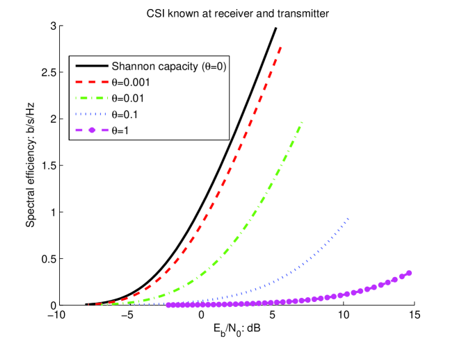
Figure 3: Spectral efficiency vs. $E_{b}/N_{0}$ in the Rayleigh fading channel with fixed $B$; CSI known at the transmitter and receiver.

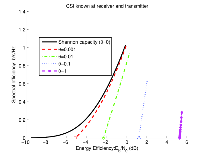
Figure 7: Spectral efficiency vs. $E_{b}/N_{0}$ in the Rayleigh fading channel with fixed $\frac{\bar{P}}{N_{0}}=10^{4}$; CSI known at the transmitter and receiver.

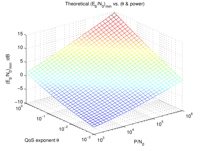
Figure 8: $\frac{E_{b}}{N_{0}}_{\min}$ vs. $\theta$ and $\bar{P}/N_{0}$ in the Rayleigh fading channel; CSI known at the transmitter and receiver.

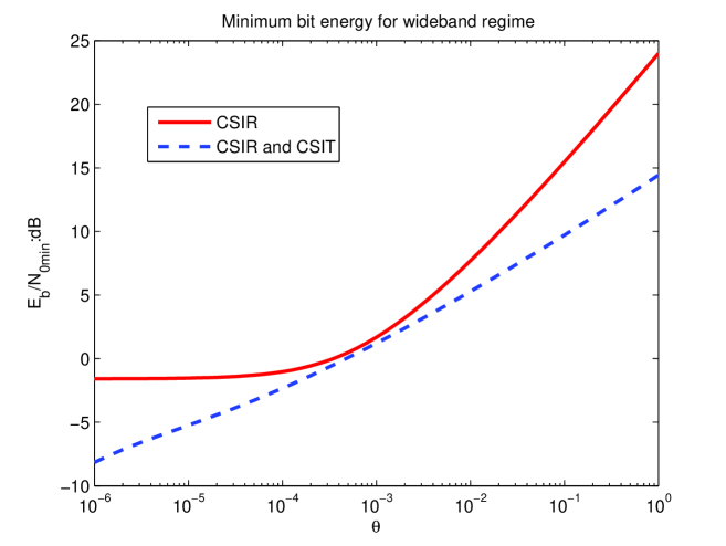
Figure 9: $\frac{E_{b}}{N_{0}}_{\min}$ vs. $\theta$ in the Rayleigh fading channel. $\frac{\bar{P}}{N_{0}}=10^{4}$.

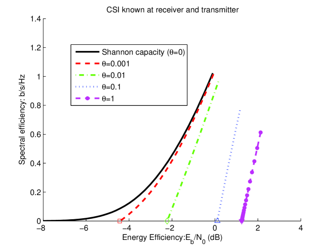
Figure 10: Spectral efficiency vs. $E_{b}/N_{0}$ in the Nakagami-$m$ fading channel with $m=2$; $\frac{\bar{P}}{N_{0}}=10^{4}$ ;CSI known at the transmitter and receiver.

References

- [1] E. Biglieri, J. Proakis, and S. Shamai (Shitz), “Fading channels: Information-theoretic and communications aspects,” IEEE Trans. Inform. Theory, vol. 44, pp. 2619-2692, Oct. 1998.
- [2] S. Verd, “Spectral efficiency in the wideband regime,” IEEE Trans. Inform. Theory, vol.48, no.6 pp.1319-1343. Jun.2002.
- [3] A. Ephremides and B. Hajek, “Information theory and communication networks: An unconsummated union,” IEEE Trans. Inform. Theory, vol. 44, pp. 2416-2434, Oct. 1998.
- [4] L. Ozarow, S. Shamai (Shitz), and A. Wyner, “Information theoretic considerations for cellular mobile radio,” IEEE Trans. Veh. Technol., vol. 43, pp. 359-378, May 1994.
- [5] S. V. Hanly and D.N.C Tse, “Multiaccess fading channels-part II: delay-limited capacities,” IEEE Trans. Inform. Theory, vol.44, no.7, pp.2816-2831. Nov. 1998.
- [6] I. E. Telatar and R. G. Gallager, “Combining queueing theory with information theory for multiaccess,” IEEE J. Select. Areas Commun., vol. 13, pp. 963-969, Aug. 1995.
- [7] R. A. Berry and R. G. Gallager, “Communication over fading channels with delay constraints,” IEEE Trans. Inform. Theory, vol. 48, pp. 1135-1149, May 2002.
- [8] M. J. Neely, “Optimal energy and delay tradeoffs for multiuser wireless downlinks,” IEEE Trans. Inform. Theory, vol. 53, pp. 3095-3113, Sept. 2007.
- [9] F. Kelly, “Notes on effective bandwidths,” Stochastic Networks: Theory and Applications, Royal Statistical Society Lecture Notes Series, 4., pp: 141-168, Oxford University Press, 1996.
- [10] C.-S. Chang, “Stability, queue length, and delay of deterministic and stochastic queuing networks,” IEEE Trans. Auto. Control, vol. 39, no. 5, pp. 913-931, May 1994.
- [11] C.-S. Chang, “Effective bandwidth in high-speed digital networks,” IEEE J. Sel. Areas Commun., vol.13, pp. 1091-1100, Aug. 1995.
- [12] C.-S. Chang and T. Zajic, “Effective bandwidths of departure processes from queues with time varying capacities,” INFOCOM, 1995.
- [13] D. Wu and R. Negi “Effective capacity: a wireless link model for support of quality of service,” IEEE Trans. Wireless Commun., vol.2,no. 4, pp.630-643. July 2003.
- [14] D. Wu and R. Negi, “Effective capacity-based quality of service measures for wireless networks,” Proc. First International Conference on Broadband Networks, 2004, pp. 527-536.
- [15] D. Wu and R. Negi, “Downlink scheduling in a cellular network for quality-of-service assurance,” IEEE Trans. Veh. Technol., vol.53, no.5, pp. 1547-1557, Sep., 2004.
- [16] D. Wu and R. Negi, “Utilizing multiuser diversity for efficient support of quality of service over a fading channel,” IEEE Trans. Veh. Technol., vol.49, pp. 1073-1096, May 2003.
- [17] J. Tang and X. Zhang, “Quality-of-Service Driven Power and Rate Adaptation over Wireless Links,” IEEE Trans. Wireless Commun., vol. 6, no. 8, pp.3058-3068, Aug. 2007.
- [18] J. Tang and X. Zhang, “Quality-of-Service Driven Power and Rate Adaptation for Multichannel Communications over Wireless Links,” IEEE Trans. Wireless Commun., vol. 6, no. 12, pp.4349-4360, Dec. 2007.
- [19] J. Tang and X. Zhang, “Cross-layer modeling for quality of service guarantees over wireless links,” IEEE Trans. Wireless Commun., vol. 6, no. 12, pp.4504-4512, Dec. 2007.
- [20] J. Tang and X. Zhang, “Cross-layer-model based adaptive resource allocation for statistical QoS guarantees in mobile wireless networks,” IEEE Trans. Wireless Commun., vol. 7, pp.2318-2328, June 2008.
- [21] L. Liu, P. Parag, J. Tang, W.-Y. Chen and J.-F. Chamberland, “Resource allocation and quality of service evaluation for wireless communication systems using fluid models,” IEEE Trans. Inform. Theory, vol. 53, no. 5, pp. 1767-1777, May 2007.
- [22] S. Shamai, S. Verd, “The impact of frequency-flat fading on the spectral efficiency of CDMA,” IEEE Trans. Inform. Theory, vol. 47, no. 4, pp. 1302-1327, May 2001.
- [23] S. Borade and L. Zheng, “Wideband fading channels with feedback,” 42nd Allerton Annual Conference on Communication, Control and Computing, October 2004.
- [24] M. Luby, “LT codes,” Proc. 43rd Ann. IEEE Symp. Found. Comp. Sci., 2002, pp. 271 280.
- [25] A. Shokrollahi, “Raptor codes,” IEEE Trans. Inform. Theory, vol. 52, pp. 2551-2567, June 2006.
- [26] J. Casture and Y. Mao, “Rateless coding and relay networks,” IEEE Signal Process. Mag., vol. 24, pp. 27-35, Sept. 2007.
- [27] J. Casture and Y. Mao, “Rateless coding over fading channels,” IEEE Comm. Letters, vol. 10, pp. 46-48, Jan. 2006.
- [28] T. M. Cover and J. A. Thomas, Elements of Information Theory. New York: Wiley, 1991.
- [29] C.-S. Chang, Performance Guarantees in Communication Networks, Springer-Verlag, 2000.
- [30] S. Boyd and L. Vandenberghe, Convex Optimization, Cambridge University Press, 2004.
- [31] V. K. Garg, Wireless Communications and Networking, Elsevier, 2007.
- [32] T. S. Rappaport, Wireless Communications: Principles and Practice, 2nd ed. Prentice Hall PTR, 2001.