A novel method for computing torus amplitudes for $\mathbb{Z}_{N}$ orbifolds without the unfolding technique

Abstract:

A novel method for computing torus amplitudes in orbifold compactifications is suggested. It applies universally for every Abelian $\mathbb{Z}_{N}$ orbifold without requiring the unfolding technique. This method follows from the possibility of obtaining integrals over fundamental domains of every Hecke congruence subgroup $\Gamma_{0}[N]$ by computing contour integrals over one-dimensional curves uniformly distributed in these domains.

1 Introduction

Superstring orbifolds compactifications are among the few examples where semi-realistic physics emerges in a complete string description. By choosing an orbifold space to compactify the superstring which do not preserve any of its original supersymmetries, one can study quantum effects induced by the infinite towers of string excitations. This effects are encoded by the string free-energy given by the (worldsheet) torus amplitude. This amplitude is generically non zero after supersymmetry breaking, and plays the role of a potential in the geometric string moduli. Quantum effects induced by supersymmetry breaking include at times generation of closed string tachyons, and generically uplifting of the string moduli. The presence of closed string tachyons in regions of the moduli space induce a break-down of the analyticity of the free-energy, which signals the presence of a phase transition involving the space-time background itself. This is a non-perturbative process difficult to analyze except under very special circumstances. The non-tachyonic cases are more under control, although afflicted by the problem of moduli stabilization. Generically, the torus potential has runaway directions in the moduli space, pushing the system towards its decompactification limits. There are however examples where some or all the geometric moduli can be stabilized in local minima of the torus potential [1],[2],[3].

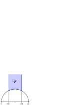
Figure 1: The standard fundamental region $\mathcal{F}=\{|\tau|>1,-1/2\leq\tau_{1}<1/2\}$ of the torus modular group $\Gamma\sim\mathop{\rm PSL}(2,\mathbb{Z})$ in the upper complex plane $\mathbb{H}$.

In order to obtain the potential in the string moduli one has to compute the torus amplitude. This is given by an integral in the complex worldsheet torus parameter $\tau$ over a fundamental region $\mathcal{F}$, (shown in figure 1) of the torus modular group $\Gamma\sim\mathop{\rm PSL}(2,\mathbb{Z})$.

For a $\mathbb{Z}_{p}$-orbifold with $p$ prime integer the torus amplitude has the following structure

$$V_{p} \sim -\int_{\mathcal{F}}\frac{d^{2}\tau}{\tau_{2}^{2}}\left(1+S+TS+...+T^{p-1}S\right)$$

$$\cdot\frac{1}{\tau_{2}^{-1+d/2}}Str_{(\mathcal{H}_{L}\times\mathcal{H}_{R})}\left(\frac{1/p+g+...+g^{p-1}}{p}q^{L_{0}-c/24}\bar{q}^{\bar{L}_{0}-\bar{c}/24}\right)$$

$$= \int_{\mathcal{F}}\frac{d^{2}\tau}{\tau_{2}^{2}}\left(1+S+TS+...+T^{p-1}S\right)\left(\frac{f_{0,0}}{p}+f_{1,0}+...+f_{p-1,0}\right)$$

where $q=e^{2i\pi\tau}$, and $d$ is the number of non-compact dimensions. $g$ is the orbifold operator with a definite action on the superstring states belonging to $\mathcal{H}_{L}\times\mathcal{H}_{R}$. $g$ generates the $\mathbb{Z}_{p}$ cyclic group ($g^{p}=1$), $\mathbb{Z}_{p}\sim\{\{0,1,...,p-1\},+(mod\ p)\}$.

In (LABEL:potential) we have used the following notation

$$f_{i,j}(\tau,\bar{\tau})=\frac{1}{p\tau_{2}^{1-d/2}}Str_{(\mathcal{H}_{L}\times\mathcal{H}_{R})_{j}}\left(g^{i}q^{L_{0}-c/24}\bar{q}^{\bar{L}_{0}-\bar{c}/24}\right),$$ (2)

for the contributions from the $j$-twisted strings with the $g^{i}$ insertion in the supertrace. All the worldsheet fields in the $j$-twisted sector satisfy the boundary conditions

$$\phi(\sigma+2\pi,t)=g^{j}\phi(\sigma,t).$$ (3)

The $g^{i}$ insertion in eq. (2) produces a twisting in the fields boundary condition along the $t$-homology cycle of the worldsheet torus.

The modular transformations in (LABEL:potential), where $T:\tau\rightarrow\tau+1$ and $S:\tau\rightarrow-1/\tau$, are required to produce new terms which complete a modular invariant multiplet. The action of the generator $S$ and $T$ on the functions $f_{i,j}(\tau,\bar{\tau})$ is given by (mod($p$))

$$S:f_{i,j}(\tau,\bar{\tau}) \rightarrow f_{-j,i}(\tau,\bar{\tau})$$

$$T:f_{i,j}(\tau,\bar{\tau}) \rightarrow f_{i+j,j}(\tau,\bar{\tau}).$$

One can check that the set of $p^{2}-1$ terms in the integral (LABEL:potential) form a modular invariant multiplet. In fact, the set of transformations $(S,TS,...,T^{p-1}S)$ by acting on each of the $T$-invariant $p-1$ terms $f_{i,0}$, generate a $(p-1)$-dimensional $T$-invariant multiplet. Terms in distinct multiplets are then connected by $S$ transformations.

By performing a change of integration variable in (LABEL:potential) one can rewrite the torus amplitude $V_{p}$ as follows

$$V_{p}\sim-\int_{\mathcal{F}_{p}}\frac{d^{2}\tau}{\tau_{2}^{2}}\left(\frac{f_{0,0}}{p}+f_{1,0}+...+f_{p-1,0}\right).$$ (4)

where $\mathcal{F}_{p}=\mathcal{F}\cup_{i=1}^{p-1}ST^{i}(\mathcal{F})$. This new integration region is a fundamental domain for the congruence subgroup $\Gamma_{0}[p]\subset\Gamma$, given by $\mathop{\rm PSL}(2,\mathbb{Z})$ matrices of the form

$$\begin{pmatrix}a&b\\ pc&pd+k\\ \end{pmatrix},$$ (5)

with $(pc,pd+k):=MCD(pc,pd+k)=1$.

In the literature computation of the $\tau$ integral over the region $\mathcal{F}_{p}$ in (4) is usually carried on by using the unfolding technique [4],[5],[6],[7],[8],[9],[10],[11]. In toroidal orbifolds for a compactification down to $d$-dimensions, lattice states given by the $d$-dimensional momentum quantum number $\vec{m}$ and the $d$-dimensional winding number $\vec{n}$ are used to unfold the $\mathcal{F}_{p}$ domain. These quantum numbers can be arranged to form a representation of a subgroup $G$ of $GL(10-d,\mathbb{Z})$. By computing the orbits of $\Gamma_{0}[p]$ in $G$, the original integral (4) on the domain $\mathcal{F}_{p}$ can be reduced to an integral over the strip $\mathcal{S}=[-1/2,1/2]\times[0,\infty)$ involving as many terms as the number of independent orbits of $\Gamma_{0}[p]$ in $G$. For a generic $\mathbb{Z}_{N}$ this method can be quite complicate to follow, and the tricks to be used to obtain the final unfolded integral depend on the dimension of the subgroup $G\subset GL(10-d,\mathbb{Z})$ [7],[11]. The general method for unfolding the integration domain for a generic $\mathbb{Z}_{N}$ orbifold is studied in [10].

Here we propose a different way for computing integrals over fundamental regions $\mathcal{F}_{p}$ of the congruence subgroups $\Gamma_{0}[p]$ of the kind of (4). Instead of unfolding $\mathcal{F}_{p}$ into the strip $\mathcal{S}$, we trade the integral over $\mathcal{F}_{p}$ for a contour integrals over a (one-dimensional) curve which is uniformly distributed in $\mathcal{F}_{p}$. Uniform distributions property of one-dimensional curves in homogenous space with negative curvature has been extensively studied in the mathematics literature [12],[13],[14],[15] and quite general theorems have been obtained.

In appendix we give our proof of a uniform distribution theorem for $\mathbb{H}/\Gamma_{0}[N]$ hyperbolic spaces based on elementary function analysis. This theorem states that for every congruence subgroup $\Gamma_{0}[N]$ with fundamental region $\mathcal{F}_{N}$ in the upper complex plane $\mathbb{H}$, there is a (one-dimensional) curve which is dense and uniformly distributed in $\mathcal{F}_{N}$. This curve appears is the image in $\mathcal{F}_{N}$ of the infinite radius horocycle in the upper hyperbolic plane $\mathbb{H}$.

A sequence of horocycles $\{h_{n}\}_{n\in\mathbb{N}}$ converging to the infinite radius horocycle, (the real axis), have their image curves $\{\gamma_{n}\}_{n\in\mathbb{N}}$ in $\mathcal{F}_{N}$ which tend to become uniform distributed in $\mathcal{F}_{N}$ for $n\rightarrow\infty$. Therefore for enough regular function $f(\tau,\bar{\tau})$

$$\lim_{n\rightarrow\infty}\frac{1}{L(\gamma_{n})}\oint_{\gamma_{n}}dsf(\tau,\bar{\tau})=\frac{1}{A(\mathcal{F}_{N})}\int_{\mathcal{F}_{N}}\frac{d^{2}\tau}{\tau_{2}^{2}}f(\tau,\bar{\tau}),$$ (6)

where $L(\gamma_{n})$ is the length of $\gamma_{n}$ computed by the hyperbolic metric

$$L(\gamma_{n})=\oint_{\gamma_{n}}ds=\oint_{\gamma_{n}}\frac{\sqrt{d\tau_{1}^{2}+d\tau_{1}^{2}}}{\tau_{2}}.$$ (7)

In eq. (6) the integral over a fundamental region $\mathcal{F}_{N}$ is normalized by the area $A(\mathcal{F}_{N})$ of the hyperbolic polygon $\mathcal{F}_{N}$.

$$A(\mathcal{F}_{N})=\int_{\mathcal{F}_{N}}\frac{d\tau_{1}d\tau_{2}}{\tau_{2}^{2}}.$$ (8)

Since the limiting curve $\gamma_{\infty}$ in (6) is the image of the infinite radius horocycle (the real axis) then for every enough regular $\Gamma_{0}[N]$-invariant function $f$

$$\int_{\mathcal{F}_{N}}\frac{d^{2}\tau}{\tau_{2}^{2}}f(\tau,\bar{\tau})=A(\mathcal{F}_{N})\lim_{\tau_{2}\rightarrow 0}\int_{-1/2}^{1/2}d\tau_{1}f(\tau,\bar{\tau}).$$ (9)

This result provides an alternative way for computing the torus amplitude (4), and more generally the torus amplitude for every $\mathbb{Z}_{N}$ orbifold, $N\in\mathbb{N}$.

The organization of the rest of the paper is the following: in the next section we start by considering specific examples such as the $\mathbb{Z}_{4}$ and $\mathbb{Z}_{6}$ orbifolds and illustrate in details the construction of the modular invariant multiplets. Then we show the equivalence of the modular integral for the torus amplitude to a $\tau_{2}\rightarrow 0$ limit of the untwisted sector partition functions, modified by coefficients depending on the dimensions of the cyclic subgroups of $\mathbb{Z}_{4}$ and $\mathbb{Z}_{6}$. We then provide the general formula for the torus amplitude, valid for a generic $\mathbb{Z}_{N}$. The proof of the uniform distribution theorem is given in the appendix.

2 The torus amplitude for a generic $\mathbb{Z}_{N}$ orbifold

2.1 The $\mathbb{Z}_{4}$ case

For a $\mathbb{Z}_{4}$ orbifold the torus amplitude has the following structure

$$V_{4}\sim\int_{\mathcal{F}}\frac{d^{2}\tau}{\tau_{2}^{2}}(1+S+TS)(1+ST^{2}S)\left(f_{1,0}+\frac{1}{2}f_{2,0}+f_{3,0}\right).$$ (10)

$f_{1,0}$ and $f_{3,0}$ are $\Gamma_{0}[4]$ invariant, while $f_{2,0}$ is invariant under the larger congruence subgroup $\Gamma_{0}[2]\supset\Gamma_{0}[4]$.

Since $(1+S+TS+T^{2}S+T^{3}S)f_{2,0}=2(f_{2,0}+f_{0,2}+f_{2,2})$, the terms $f_{1,2}$ and $f_{3,2}$ are obtained from $f_{1,0}$ and $f_{3,0}$ through a $ST^{2}S$ transformation.

By a change of integration variable, eq. (10) can be reduced to

$$V_{4}\sim\int_{\mathcal{F}_{4}}\frac{d^{2}\tau}{\tau_{2}^{2}}\left(f_{1,0}+\frac{1}{2}f_{2,0}+f_{3,0}\right),$$ (11)

where $\mathcal{F}_{4}$ is a fundamental domain for $\Gamma_{0}[4]$

$$\mathcal{F}_{4}=\mathcal{F}\cup\bigcup_{i=0}^{3}ST^{i}(\mathcal{F})\bigcup ST^{2}S(\mathcal{F}).$$ (12)

By using the uniform distribution of the infinite radius horocycle in $\mathcal{F}_{4}$ one can then express the torus potential for a generic $\mathbb{Z}_{4}$ orbifold (11) as the following $\tau_{2}\rightarrow 0$ limit

$$V_{4}\sim 6\cdot\frac{\pi}{3}\lim_{\tau_{2}\rightarrow 0}\int_{-1/2}^{1/2}d\tau_{1}\left(f_{1,0}+\frac{1}{2}f_{2,0}+f_{3,0}\right)(\tau,\bar{\tau}),$$ (13)

where the factor $6\pi/3$ is equal to the invariant area of the fundamental region $\mathcal{F}_{4}$ of $\Gamma_{0}[4]$. Notice in eq. (13) the presence of the factor $1/2$ in front of $f_{2,0}$. This is connected with the invariance of this term under the larger congruence subgroup $\Gamma_{0}[2]$. In the general formula to be given below for a $\mathbb{Z}_{N}$ orbifold when $N$ is not prime, rational coefficient will appear in front of terms which are invariant under the cyclic subgroups of $\mathbb{Z}_{N}$. Before writing the general formula we study in the next section the $\mathbb{Z}_{6}$ example.

2.2 The $\mathbb{Z}_{6}$ case

The torus amplitude is given by

$$V_{6} \sim \int_{\mathcal{F}}\frac{d^{2}\tau}{\tau_{2}^{2}}\Bigg{[}\left(1+\sum_{i=0}^{5}T^{i}S+(1+S+TS)T^{3}S+(1+S+TS+T^{2}S)T^{4}S\right)(f_{1,0}+f_{5,0})$$ (14)

$$+ (1+S+TS+T^{2}S)(f_{2,0}+f_{4,0})+(1+S+TS)f_{3,0}\Bigg{]}.$$

The above structure follows from the $\Gamma_{0}[3]$ invariance of $(f_{2,0}+f_{4,0})$, and the $\Gamma_{0}[2]$ invariance of $f_{3,0}$.

The amplitude can be rewritten as

$$V_{6}\sim\int_{\mathcal{F}_{6}}\frac{d^{2}\tau}{\tau_{2}^{2}}(f_{1,0}+f_{5,0})+\int_{\mathcal{F}_{3}}\frac{d^{2}\tau}{\tau_{2}^{2}}(f_{2,0}+f_{4,0})+\int_{\mathcal{F}_{2}}\frac{d^{2}\tau}{\tau_{2}^{2}}f_{3,0}.$$ (15)

By using uniform distribution property one can express the same amplitude as the following limit

$$V_{6}\sim 12\cdot\frac{\pi}{3}\lim_{\tau_{2}\rightarrow 0}\int_{-1/2}^{1/2}d\tau_{1}\left(f_{1,0}+\frac{1}{3}f_{2,0}+\frac{1}{4}f_{3,0}+\frac{1}{3}f_{4,0}+f_{5,0}\right),$$ (16)

where $12\pi/3$ is the hyperbolic area of a fundamental region of $\Gamma_{0}[6]$.

2.3 Amplitude for a generic $\mathbb{Z}_{N}$ orbifold

The analysis in the previous section for the $\mathbb{Z}_{4}$ and $\mathbb{Z}_{6}$ orbifolds suggests the way for obtaining a decomposition of a generic $\mathbb{Z}_{N}$ torus amplitude as a sum of integrals over fundamental regions of congruence subgroups $\Gamma_{0}[q]$, $2\leq q\leq N$. This decomposition together with the theorem on uniform distribution gives the following formula for the torus amplitude in a non-tachyonic $\mathbb{Z}_{N}$ orbifold

$$V_{N}\sim\lim_{\tau_{2}\rightarrow 0}\int_{-1/2}^{1/2}d\tau_{1}\sum_{l=1}^{N-1}A\left(\mathcal{F}_{n(l)}\right)f_{l,0}(\tau,\bar{\tau}),$$ (17)

where the integer numbers $0<n(l)<N$ are solutions of the following equation

$$l\cdot n(l)=N,\ \ mod(N),$$ (18)

and $A(\mathcal{F}_{r})$ is the area of the fundamental region $\mathcal{F}_{r}$ of the congruence subgroup $\Gamma_{0}[r]$ which can be computed by

$$A(\mathcal{F}_{r})=\frac{2r^{2}}{\pi\varphi(r)}\sum_{(k,r)=1}\sum_{n=0}^{\infty}\frac{1}{(rn+k)^{2}}.$$ (19)

In the last formula $\varphi(r)$ is the Euler totient phi-function, which counts the number of integers $k$, $1\leq k<r$ coprime with $r$, $(k,r)=1$. Given the $r$ decomposition in prime factors $r=p_{1}^{s_{1}}\cdot...\cdot p_{q}^{s_{q}}$, $\varphi(r)$ can be computed by the following Euler product

$$\varphi(r)=\prod_{p|r}\left(1-\frac{1}{p}\right),$$ (20)

where $p|r$ indicates that $p$ is a divisor of $r$.

In equation (18) if $l$ is coprime with $N$, $(l,N)=1$, then $n(l)=N$ and $g^{l}$ generates the full $\mathbb{Z}_{N}$. If $(l,N)>1$ then $n(l)$ is the common factor between $l$ and $N$, $n(l)<N$, and $g^{l}$ generates the cyclic subgroup $\mathbb{Z}_{n(l)}\subset\mathbb{Z}_{N}$. In this last case the untwisted terms $f_{l,0}(\tau,\bar{\tau})$, are invariant under the congruence subgroup $\Gamma_{0}[n(l)]$, with fundamental domain $\mathcal{F}_{n(l)}$. This was the case for the unwisted terms which appeared dressed by fractional coefficients for the $\mathbb{Z}_{4}$ orbifold in eq. (13) and for the $\mathbb{Z}_{6}$ orbifold in eq. (16). This fractional coefficients are the ratios $A(\mathcal{F}_{n(l)})/A(\mathcal{F}_{N})$ of the areas of the fundamental regions of $\Gamma_{0}[n(l)]$ and $\Gamma_{0}[N]$, which are rational numbers since every congruence subgroup is covered by a finite number of fundamental regions of $\Gamma$.

Appendix A Uniform distribution of curves in the fundamental regions of the Hecke congruence subgroups

For every integer $N>1$, the congruence subgroup $\Gamma_{0}[N]\subset\Gamma$ is represented by matrices in $\mathop{\rm PSL}(2,\mathbb{Z})$ with $c=0$, (mod $N$). These matrices have the form

$$\begin{pmatrix}a&b\\ Nc&Nd+k\\ \end{pmatrix},$$ (21)

with $(Nc,Nd+k)=1$.

A Fundamental region of $\Gamma_{0}[N]$ on the hyperbolic upper plane $\mathcal{F}_{N}=\mathbb{H}/\Gamma_{0}[N]$ is given by the union of a fundamental region $\mathcal{F}$ of the full modular group $\Gamma$ with the images of $\mathcal{F}$ through all the transformations in $(\Gamma-\Gamma_{0}[N])/T$. $\mathcal{F}_{N}$ is an hyperbolic polygon whose vertexes in $z=i\infty$ and in points in $\mathbb{Q}\cup[-1/2,1/2]$ are called cusps, (the fundamental region $\mathcal{F}_{2}$ of $\Gamma_{0}[2]$ is shown in figure 2.)

Here we prove that for every congruence subgroup $\Gamma_{0}[N]\subset\Gamma$, the image of the infinite radius horocycle through $\Gamma_{0}[N]$ transformations is uniformly distributed in the fundamental region $\mathcal{F}_{N}=\mathbb{H}/\Gamma_{0}[N]$. To this purpose we will show that for every regular enough $\Gamma_{0}[N]$ invariant function $f(\tau,\bar{\tau})$

$$\frac{1}{L(\gamma_{\infty})}\oint_{\gamma_{\infty}^{N}}dsf=\lim_{\tau_{2}\rightarrow 0}\int_{-1/2}^{1/2}d\tau_{1}f\rightarrow\frac{1}{A(\mathcal{F}_{n})}\int_{\mathcal{F}_{N}}\frac{d\tau_{1}d\tau_{2}}{\tau_{2}^{2}}f,$$ (22)

where the upper plane $\mathbb{H}$ hyperbolic metric is given by

$$ds^{2}=\frac{d\tau_{1}^{2}+d\tau_{2}^{2}}{\tau_{2}^{2}}.$$ (23)

In eq. (22) $\gamma_{\infty}^{N}\subset\mathcal{F}_{N}$ denotes the image curve of the infinite radius horocycle, and $L(\gamma)$ denotes the hyperbolic length of a curve $\gamma$

$$L(\gamma)=\oint_{\gamma}ds=\oint_{\gamma}\frac{\sqrt{d\tau_{1}^{2}+d\tau_{2}^{2}}}{\tau_{2}}.$$ (24)

• i) Let $f(\tau,\bar{\tau})$ be a function invariant under $\Gamma_{0}[N]$, finite over the fundamental domain $\mathcal{F}_{N}$ of $\Gamma_{0}[N]$, except possibly at the cusps of $\mathcal{F}_{N}$, which include $\tau=i\infty$ and points in $\mathbb{Q}\cap[-1/2,1/2]$.

• ii) Let the integral on $\mathcal{F}_{N}$ of $f(\tau,\bar{\tau})$ be convergent

  $$\left|\int_{\mathcal{F}_{N}}\frac{d^{2}\tau}{\tau_{2}^{2}}f(\tau,\bar{\tau})\right|<\infty.$$ (25)

• iii) $f$ has the following Fourier expansion

  $$f(q,\bar{q})=\sum_{i=1}^{n_{c}(N)}\frac{c_{i}}{q-e^{2\pi i\tau_{i}}}+regulars,$$ (26)

  where $q=e^{2\pi i\tau}$, $n_{c}(N)$ is the number of cusps of $\mathcal{F}_{N}$, and $\tau_{i}$ the locations of the cusps.

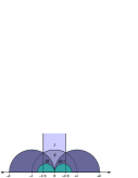
Figure 2: The region $I\cup S\cup ST$ is a fundamental domain for $\Gamma_{0}[2]$

Then:

$$\int_{\mathcal{F}_{N}}\frac{d^{2}\tau}{\tau_{2}^{2}}f(\tau,\bar{\tau})=A(\mathcal{F}_{N})\lim_{\tau_{2}\rightarrow 0}\int_{-1/2}^{1/2}d\tau_{1}f(\tau,\bar{\tau})+24\frac{\pi}{3}\sum_{i=1}^{n_{c}(N)}c_{i}\beta_{i},$$ (27)

where in the above equation

$$A(\mathcal{F}_{N})=\frac{2N^{2}}{\pi\varphi(N)}\sum_{(k,N)=1}\sum_{n=0}^{\infty}\frac{1}{(nN+k)^{2}}.$$ (28)

is the modular invariant area of the fundamental region $\mathcal{F}_{N}$ of $\Gamma_{0}[N]$, and $\beta_{i}$ is the number of fundamental regions of the full modular group $\Gamma$ in the tassellation of $\mathcal{F}_{N}$ which have the same cusp $\tau_{i}$ . In eq. (28) $\varphi(N)$ is the Euler totient phi-function.

Proof.

We consider the following $\Gamma_{0}[N]$-invariant auxiliary function

$$h_{N}(\tau,R)=\sum_{(k,N)=1}^{N-1}\sum_{m=-\infty}^{\infty}\sum_{n=-\infty}^{\infty}e^{-\frac{\pi R^{2}}{N^{2}\tau_{2}}|nN\tau+mN+k|^{2}}.$$ (29)

By using Poisson resummation formula one can prove the following

$$\sum_{m=-\infty}^{\infty}\sum_{n=-\infty}^{\infty}e^{2\pi imk/N}e^{-\frac{\pi}{R^{2}\tau_{2}}|n\tau+m|^{2}}=R^{2}\sum_{m=-\infty}^{\infty}\sum_{n=-\infty}^{\infty}e^{-\frac{\pi R^{2}}{N^{2}\tau_{2}}|nN\tau+mN+k|^{2}}.$$ (30)

From the previous two relation by taking the limit $R\rightarrow 0$ one obtains the following identity

$$\frac{1}{\varphi(N)}\lim_{R\rightarrow 0}R^{2}\sum_{(k,N)=1}^{N-1}\sum_{m=-\infty}^{\infty}\sum_{n=-\infty}^{\infty}e^{-\frac{\pi R^{2}}{p^{2}\tau_{2}}|nN\tau+mN+k|^{2}}=1.$$ (31)

By using the previous identity one therefore has

$$\int_{\mathcal{F}_{N}}\frac{d^{2}\tau}{\tau_{2}^{2}}f(\tau,\bar{\tau})=\frac{1}{\varphi(N)}\lim_{R\rightarrow 0}R^{2}\int_{\mathcal{F}_{N}}\frac{d^{2}\tau}{\tau_{2}^{2}}f(\tau,\bar{\tau})\sum_{m=-\infty}^{\infty}\sum_{n=-\infty}^{\infty}\sum_{(k,N)=1}^{N-1}e^{-\frac{\pi R^{2}}{N^{2}\tau_{2}}|nN\tau+mN+k|^{2}}.$$ (32)

Let us decompose $nN=(Nr+s)Nc$ and $mN+k=(Nr+s)(Nd+k^{\prime})$ where $Nr+s=(nN,mn+k)$ and therefore (N,s)=1 with $1\leq s\leq N-1$. $Nc$ and $Nd+k^{\prime}$ are therefore coprime $(Nc,Nd+k^{\prime})=1$.

With the above decomposition (32) becomes

$$\int_{\mathcal{F}_{N}}\frac{d^{2}\tau}{\tau_{2}^{2}}f(\tau,\bar{\tau})=\frac{1}{\varphi(N)}\lim_{R\rightarrow 0}R^{2}\int_{\mathcal{F}_{N}}\frac{d^{2}\tau}{\tau_{2}^{2}}f(\tau,\bar{\tau})\sum_{(s,N)=1}^{N-1}\sum_{r=-\infty}^{\infty}\sum_{c,d\in\mathbb{Z}}\sum_{(k,N)=1}^{N-1}e^{-\pi R^{2}(Nr+s)^{2}\frac{|Nc\tau+Nd+k|^{2}}{N^{2}\tau_{2}}}.$$ (33)

Notice at the exponent the images of $\tau_{2}$ under $\Gamma_{0}[N]$ transformations. In fact, under a generic $\Gamma_{0}[N]$ transformation given by a matrix with lower row $(Nc,\ \ Nd+k)$, $\tau_{2}$ is mapped to

$$\tau_{2}\rightarrow\frac{\tau_{2}}{|Nc\tau+Nd+k|^{2}}.$$ (34)

Moreover, since left multiplication by $T^{q}$, $q\in\mathbb{Z}$ of a generic $\Gamma_{0}[N]$ matrix leaves its lower row invariant

$$T^{q}\begin{pmatrix}a&b\\ Nc&Nd+k\\ \end{pmatrix}=\begin{pmatrix}1&q\\ 0&1\\ \end{pmatrix}\begin{pmatrix}a&b\\ Nc&Nd+k\\ \end{pmatrix}=\begin{pmatrix}a^{\prime}&b^{\prime}\\ Nc&Nd+k\\ \end{pmatrix},$$ (35)

the set of $\Gamma_{0}[N]$ matrixes at the exponent in (33) form twice a representation of $\Gamma_{0}[N]/T$.

For a given $c$,$d$ and $k$ we call $M_{c,d,k}$

$$M_{c,d,k}=\begin{pmatrix}a&b\\ Nc&Nd+k\\ \end{pmatrix},$$ (36)

the matrix which maps $\tau\in\mathcal{F}_{N}$ into a point $M_{c,d,k}\tau\in\mathcal{S}-\mathcal{F}_{N}$, where $\mathcal{S}=[-1/2,1/2]\times[0,\infty)$.

By changing integration variable $\tau\rightarrow M_{c,d,k}^{-1}\tau$ in the generic term in the r.h.s. of (32) one finds

$$\int_{\mathcal{F}_{N}}\frac{d^{2}\tau}{\tau_{2}^{2}}f(\tau,\bar{\tau})e^{-\frac{\pi R^{2}(Nr+s)^{2}}{N^{2}\tau_{2}}|Nc\tau+Nd+k|^{2}}=\int_{M_{c,d,k}(\mathcal{F}_{N})}\frac{d^{2}\tau}{\tau_{2}^{2}}f(\tau,\bar{\tau})e^{-\frac{\pi(Nr+s)^{2}R^{2}}{N^{2}\tau_{2}}}.$$ (37)

The union of all the $\{M_{c,d,k}\}$ span twice the coset $\Gamma_{0}[N]/T$, and therefore

$$\mathcal{F}_{N}\cup\bigcup_{c,d,k}M_{c,d,k}(\mathcal{F}_{N})$$ (38)

is a double tassellation of the strip $\mathcal{S}=[-1/2,1/2]\times[0,\infty)$, whose tiles are an infinite set of fundamental regions of $\Gamma_{0}[N]$.

Thus by changing integration variable $\tau\rightarrow M_{c,d,k}^{-1}\tau$ term by term in the r.h.s. of eq. (33), one should recover

$$\int_{\mathcal{F}_{N}}\frac{d^{2}\tau}{\tau_{2}^{2}}f(\tau,\bar{\tau}) = \frac{2}{\varphi(N)}\lim_{R\rightarrow 0}R^{2}\int_{0}^{\infty}\frac{d\tau_{2}}{\tau_{2}^{2}}\int_{-1/2}^{1/2}d\tau_{1}f(\tau,\bar{\tau})\sum_{(s,N)=1}^{N-1}\sum_{r=-\infty}^{\infty}e^{-\frac{\pi R^{2}(Nr+s)^{2}}{N^{2}\tau_{2}}}$$

$$= \frac{2}{L(S^{1}(\tau_{2}))\varphi(N)}\lim_{R\rightarrow 0}R^{2}\int_{0}^{\infty}d\tau_{2}\oint_{S^{1}(\tau_{2})}dsf(\tau,\bar{\tau})\sum_{(s,N)=1}^{N-1}\sum_{r=-\infty}^{\infty}e^{-\frac{\pi R^{2}(Nr+s)^{2}}{N^{2}\tau_{2}}},$$

where $S^{1}(\tau_{2})$ is the circle $S^{1}(\tau_{2})=\{-1/2\leq x<1/2,\ y=\tau_{2}\}\subset\mathbb{H}/T$.

Notice that the length of $S^{1}(\tau_{2})$, $L(S^{1}(\tau_{2}))=1/\tau_{2}$ becomes infinite as $\tau_{2}\rightarrow 0$ due to the hyperbolic metric $ds=\sqrt{d\tau_{1}^{2}+d\tau_{2}^{2}}/\tau_{2}$ of $\mathbb{H}$.

In the Laurent expansion iii) for $f$, the simple poles in the cusps $q=0$ and on some points of the circle $|q|=1$ may spoil eq. (LABEL:unfolded2). This is best seen for a divergence at the cusp $q=0$, ($\tau=i\infty$). In fact, the integral of $f$ on the region (figure 1) $\mathcal{F}\subset\mathcal{F}_{N}$ which extends to $\tau=\infty$ is convergent only with the prescription to perform the $\tau_{1}$ integral first, which eliminates $1/q$.

Since in the limit $\tau_{2}\rightarrow\infty$ the exponential factor in (32) behaves as

$$e^{-\frac{\pi R^{2}}{N^{2}\tau_{2}}|nN\tau+mN+k|^{2}}\sim e^{-\pi R^{2}n^{2}\tau_{2}},$$ (40)

the integral in the first line of the following equation

$$\int_{\mathcal{F}_{N}}\frac{d^{2}\tau}{\tau_{2}^{2}}f(\tau,\bar{\tau}) = \frac{1}{\varphi(N)}\lim_{R\rightarrow 0}R^{2}\int_{\mathcal{F}_{N}}\frac{d^{2}\tau}{\tau_{2}^{2}}f(\tau,\bar{\tau})\sum_{m=-\infty}^{\infty}\sum_{n=-\infty}^{\infty}\sum_{(k,N)=1}^{N-1}e^{-\frac{\pi R^{2}}{N^{2}\tau_{2}}|nN\tau+mN+k|^{2}}$$ (41)

$$= \frac{2}{\varphi(N)}\lim_{R\rightarrow 0}R^{2}\int_{0}^{\infty}d\tau_{2}\int_{-1/2}^{1/2}d\tau_{1}f(\tau,\bar{\tau})\sum_{(s,N)=1}^{N-1}\sum_{r=-\infty}^{\infty}e^{-\frac{\pi R^{2}(Nr+s)^{2}}{N^{2}\tau_{2}}}$$

is actually absolutely convergent for $\tau_{2}\rightarrow\infty$ for large enough $R>R_{0}$, (the asymptotic factor (40) for $R$ large enough cancels the exponential growing factor $1/|q|=e^{2\pi\tau_{2}}$ in the Fourier expansion of $f(\tau,\bar{\tau})$ allowed by condition iii)).

However, in order to take the limit for $R\rightarrow 0$, one needs equation (41) to hold until $R>0$ and not just for $R>R_{0}$. The validity of eq. (41) on the full semi-axis $R>0$ can be checked by considering eq. (41) for complex $R$.

By using Poisson resummation formula on the first line of of (41), one can rewrite this equation in the following equivalent way

$$\int_{\mathcal{F}_{N}}\frac{d^{2}\tau}{\tau_{2}^{2}}f(\tau,\bar{\tau}) = \frac{1}{\varphi(N)}\lim_{R\rightarrow 0}R\int_{\mathcal{F}_{N}}\frac{d^{2}\tau}{\tau_{2}^{3/2}}f(\tau,\bar{\tau})\sum_{(k,N)=1}^{p-1}\sum_{m,n}e^{2\pi ikm/N}e^{2\pi imn\tau_{1}}e^{-\pi\tau_{2}\left(\frac{m^{2}}{R^{2}}+n^{2}R^{2}\right)}$$

$$= \frac{2}{\varphi(N)}\lim_{R\rightarrow 0}R^{2}\int_{0}^{\infty}d\frac{\tau_{2}}{\tau_{2}^{2}}\int_{-1/2}^{1/2}d\tau_{1}f(\tau,\bar{\tau})\sum_{(s,r)=1}^{N-1}\sum_{r=-\infty}^{\infty}e^{-\frac{\pi R^{2}(Nr+s)^{2}}{N^{2}\tau_{2}}}.$$

The function in the first line of (LABEL:unfolded3) is analytic in the complex variable $R$ on a region where the integral converges as well as all its $R$-derivatives. A breakdown of analyticity in $R$ happens whenever in the Fourier expansion of the full integrand function there is a point $R=\bar{R}$ where a term non-exponentially suppressed for $\tau_{2}\rightarrow\infty$ appears. By taking enough $R$-derivatives one would find a divergence in the integral for $\tau_{2}\rightarrow\infty$ in such a point .

Since the factor at the exponent in the first line of (LABEL:unfolded3) for both $m$ and $n$ non-zero satisfies

$$\frac{m^{2}}{R^{2}}+n^{2}R^{2}\geq 2|mn|\geq 2,$$ (43)

indeed terms proportional to $1/q$ in the Laurent expansion for $f$ do spoil analiticity in the point $R=1$, and invalidate (41) for $0<R\leq 1$.

In order to avoid this problem we regularize the $f(\tau,\bar{\tau})$ at the cusps in a $\Gamma_{0}[N]$ invariant way. For example at the cusp $\tau=\infty$ we regularize $f\rightarrow\tilde{f}_{\infty}$ as follows

$$\tilde{f}_{\infty}(q,\bar{q})=f(q,\bar{q})-c_{\infty}J(q),$$ (44)

where $J(q)$ is the Klein modular invariant function with Laurent expansion

$$J(q)=\frac{1}{q}+196884q+21493760q^{2}+...=\frac{1}{q}+\sum_{n=1}^{\infty}a_{n}q^{n}.$$ (45)

For a simple pole at a cusp $\tau_{i}\in\mathbb{Q}\cap[-1/2,1/2]$, $f$ is regularized for $q\rightarrow e^{2\pi i\tau_{i}}$ by

$$\tilde{f}_{\tau_{i}}(q,\bar{q})=f(q,\bar{q})-\beta_{i}c_{i}J(q).$$ (46)

Since $J(q)$ has a simple pole at the cusp $\tau=\infty$, by modular invariance it has simple poles in all the images of $\tau=\infty$ through modular transformations. In particular $J(q)$ has simple poles in all the rational points in $[-1/2,1/2]$.

Moreover, $J(q)$ being holomorphic in $q$, it gives zero when integrated in $\tau_{1}$ on the interval $[-1/2,1/2]$. Therefore it doesn’t contribute to the integral along the one-dimensional curve, while its contribution over a fundamental domain of $\mathcal{F}$ is

$$\int_{\mathcal{F}}\frac{d^{2}\tau}{\tau_{2}^{2}}J(\tau)=-24\frac{\pi}{3}.$$ (47)

Moreover, since

$$\int_{-1/2}^{1/2}d\tau_{1}J(\tau)=0$$ (48)

for every $\tau_{2}$, the $J$ integral over $\mathcal{F}$ receives contribution only from the region $\aleph=\mathcal{F}-[-1/2,1/2]\times[1,\infty)$

$$\int_{\mathcal{F}}\frac{d^{2}\tau}{\tau_{2}^{2}}J(\tau)=\int_{\aleph}\frac{d^{2}\tau}{\tau_{2}^{2}}J(\tau)=-24\frac{\pi}{3}.$$ (49)

Interesting enough, from the string theory point of view $\aleph$ is the subregion of $\mathcal{F}$ where level matching is not enforced. This is a peculiar characteristic of string theory, since in field theory the proper time integration domain would have a rectangular shape.

Since eq. (LABEL:unfolded2) is valid for $\tilde{f}$ up to $R=0$, one change of integration variable $\tau_{2}\rightarrow R^{2}\tau_{2}$ and finally compute the $R\rightarrow 0$ limit

$$\int_{\mathcal{F}_{N}}\frac{d^{2}\tau}{\tau_{2}^{2}}\tilde{f}(\tau,\bar{\tau}) = \frac{1}{\varphi(N)}\lim_{R\rightarrow 0}\int_{0}^{\infty}\frac{d\tau_{2}}{\tau_{2}^{2}}\oint_{S^{1}(R^{2}\tau_{2})}\frac{ds}{L(S^{1}(R^{2}\tau_{2}))}\tilde{f}(\tau,\bar{\tau})\sum_{(s,N)=1}^{N-1}\sum_{r=-\infty}^{\infty}e^{-\frac{\pi(Nr+s)^{2}}{N^{2}\tau_{2}}}$$

$$= \frac{1}{\varphi(N)}\lim_{R\rightarrow 0}\oint_{S^{1}(R^{2})}\frac{ds}{L(S^{1}(R^{2}))}\tilde{f}(\tau,\bar{\tau})\int_{0}^{\infty}dx\sum_{(s,N)=1}^{N-1}\sum_{r=-\infty}^{\infty}e^{-\frac{\pi(Nr+s)^{2}x}{N^{2}}}$$

$$= \frac{2N^{2}}{\pi\varphi(N)}\left(\sum_{(s,N)=1}^{N-1}\sum_{n=0}^{\infty}\frac{1}{(Nn+s)^{2}}\right)\lim_{R\rightarrow 0}\frac{1}{L(S^{1}(R^{2}))}\oint_{S^{1}(R^{2})}ds\tilde{f}(\tau,\bar{\tau})$$

$$= \frac{2N^{2}}{\pi\varphi(N)}\left(\sum_{(s,N)=1}^{N-1}\sum_{n=0}^{\infty}\frac{1}{(Nn+s)^{2}}\right)\lim_{\tau_{2}\rightarrow 0}\int_{-1/2}^{1/2}d\tau_{1}\tilde{f}(\tau,\bar{\tau}).$$

By using

$$\int_{\mathcal{F}_{N}}\frac{d^{2}\tau}{\tau_{2}^{2}}\tilde{f}(\tau,\bar{\tau})=\int_{\mathcal{F}_{N}}\frac{d^{2}\tau}{\tau_{2}^{2}}f(\tau,\bar{\tau})-24\frac{\pi}{3}\sum_{i=1}^{n_{c}(N)}c_{i}\beta_{i},$$ (51)

and

$$\int_{-1/2}^{1/2}d\tau_{1}J(\tau)=0,$$ (52)

one finally recovers

$$\int_{\mathcal{F}_{N}}\frac{d^{2}\tau}{\tau_{2}^{2}}f(\tau,\bar{\tau})=\frac{2N^{2}}{\pi\varphi(N)}\left(\sum_{(s,N)=1}^{N-1}\sum_{n=0}^{\infty}\frac{1}{(Nr+s)^{2}}\right)\lim_{\tau_{2}\rightarrow 0}\int_{-1/2}^{1/2}d\tau_{1}f(\tau,\bar{\tau})+24\frac{\pi}{3}\sum_{i=1}^{n_{c}(N)}c_{i}\beta_{i},$$ (53)

which proves the theorem.

The numerical factor in front of the limit in (LABEL:final), when $N$ is prime $N=p$ is given by

$$\frac{2p^{2}}{\pi\varphi(p)}\sum_{(s,p)=1}^{p-1}\sum_{n=0}^{\infty}\frac{1}{(Nn+s)^{2}}=\frac{2p^{2}}{\pi(p-1)}\sum_{s=1}^{p-1}\sum_{n=0}^{\infty}\frac{1}{(Nn+s)^{2}}$$

$$= \frac{2p^{2}}{\pi(p-1)}\sum_{n=1}^{\infty}\left(\frac{1}{n^{2}}-\frac{1}{(pn)^{2}}\right)$$

$$= =\frac{2p^{2}}{\pi(p-1)}\left(1-\frac{1}{p^{2}}\right)\sum_{n=1}^{\infty}\frac{1}{n^{2}}=(p+1)\frac{\pi}{3}.$$

$(p+1)\pi/3$ is the invariant area of the region $\mathcal{F}_{p}$ since $\mathcal{F}_{p}=\mathcal{F}\cup\bigcup_{i=0}^{p-1}ST^{i}(\mathcal{F})$, for prime $p$. Therefore one expects for generic $N$ the following series to compute the area of the fundamental region of $\mathcal{F}_{N}$

$$A(\mathcal{F}_{N})=\frac{2N^{2}}{\pi\varphi(N)}\sum_{(s,N)=1}^{N-1}\sum_{n=0}^{\infty}\frac{1}{(Nn+s)^{2}}.$$ (55)

For every positive integer $N$, $\Gamma_{0}[N]\subset\Gamma$, and therefore $\mathcal{F}=\mathbb{H}/\Gamma\subset\mathcal{F}_{N}=\mathbb{H}/\Gamma_{0}[N]$. Indeed, the fundamental region $\mathcal{F}_{N}$ is tassellated by a finite number $\mathcal{N}(N)$ of fundamental regions of $\Gamma$, each region with invariant area $\pi/3$.

Therefore from eq. (55) one obtains the number of $\mathcal{F}$-tiles $\mathcal{N}(N)\in\mathbb{N}$ needed to cover $\mathcal{F}_{N}$

$$\mathcal{N}(N)=\frac{A(\mathcal{F}_{N})}{A(\mathcal{F})}=\frac{6N^{2}}{\pi^{2}\varphi(N)}\sum_{(s,N)=1}^{N-1}\sum_{n=0}^{\infty}\frac{1}{(Nn+s)^{2}}.$$ (56)

The sequence $\{\mathcal{N}(N)\}_{N}$ starts with

$$\{1,3,4,6,6,12,8,12,12,18,12,24,14,24,24,18,36,20,36,...\}.$$

$\mathcal{N}(N)$ drops down in correspondence of prime numbers, $\mathcal{N}(p)\leq\mathcal{N}(p-1)$ for $p$ prime. In fact the congruence subgroups for prime numbers are larger then the non-prime adjacent ones, and this difference becomes more relevant for large $N$.

References

- [1] C. Angelantonj, M. Cardella and N. Irges, “An Alternative for Moduli Stabilisation,” Phys. Lett. B 641, 474 (2006) [arXiv:hep-th/0608022].
- [2] M. Dine, A. Morisse, A. Shomer and Z. Sun, “IIA moduli stabilization with badly broken supersymmetry,” JHEP 0807, 070 (2008) [arXiv:hep-th/0612189].
- [3] C. Angelantonj, C. Kounnas, H. Partouche and N. Toumbas, “Resolution of Hagedorn singularity in superstrings with gravito-magnetic fluxes,” Nucl. Phys. B 809, 291 (2009) [arXiv:0808.1357 [hep-th]].
- [4] B. McClain and B. D. B. Roth, Modular Invariance For Interacting Bosonic Strings At Finite Temperature, Commun. Math. Phys. 111 (1987) 539.
- [5] K. H. O fBrien and C. I. Tan, Modular Invariance Of Thermopartition Function And Global Phase Structure Of Heterotic String, Phys. Rev. D36 (1987) 1184.
- [6] H. Itoyama and T. R. Taylor, Supersymmetry Restoration In The Compactified O(16) O (16) Heterotic String Theory, Phys. Lett. B186 (1987) 129.
- [7] L. J. Dixon, V. Kaplunovsky and J. Louis, Moduli dependence of string loop corrections to gauge coupling constants, Nucl. Phys. B355 (1991) 649.
- [8] P. Mayr and S. Stieberger, Threshold corrections to gauge couplings in orbifold compactifications, Nucl. Phys. B407 (1993) 725 [arXiv:hep-th/9303017].
- [9] D. M. Ghilencea, H. P. Nilles and S. Stieberger, Divergences in Kaluza-Klein models and their string regularization, New J. Phys. 4 (2002) 15 [arXiv:hep-th/0108183].
- [10] M. Trapletti, On the unfolding of the fundamental region in integrals of modular invariant amplitudes, JHEP 0302 (2003) 012 [arXiv:hep-th/0211281].
- [11] E. Kiritsis, C. Kounnas, P. M. Petropoulos and J. Rizos, String threshold corrections in models with spontaneously broken supersymmetry, Nucl. Phys. B540 (1999) 87 [arXiv:hepth/ 9807067].
- [12] H. Furstenberg, The Unique Ergodicity of the Horocycle Flow, Recent Advances in Topological Dynamics, A. Beck (ed.), Springer Verlag Lecture Notes, 318 (1972), 95-115.
- [13] S. G. Dani and J. Smillie, Uniform distribution of horocycle orbits for Fuchsian groups. Duke Math. J. 51 (1984), 185 194.
- [14] M. Ratner, Distribution rigidity for unipotent actions on homogeneous spaces. Bull. Amer. Math. Soc. (N.S.) Volume 24, Number 2 (1991), 321-325.
- [15] M. Ratner, Raghunathan s topological conjecture and distributions of unipotent flows. Duke Math. J. Volume 63, Number 1 (1991), 235-280.
- [16] D. Kutasov and N. Seiberg, “Number Of Degrees Of Freedom, Density Of States And Tachyons In String Theory And Cft,” Nucl. Phys. B 358, 600 (1991).
- [17] D. Kutasov, “Some properties of (non)critical strings,” arXiv:hep-th/9110041.
- [18] K. R. Dienes, M. Moshe and R. C. Myers, “String Theory, Misaligned Supersymmetry, And The Supertrace Constraints,” Phys. Rev. Lett. 74, 4767 (1995) [arXiv:hep-th/9503055].
- [19] K. R. Dienes, “Modular invariance, finiteness, and misaligned supersymmetry: New constraints on the numbers of physical string states,” Nucl. Phys. B 429, 533 (1994) [arXiv:hep-th/9402006].
- [20] G. W. Moore, “Atkin-Lehner Symmetry,” Nucl. Phys. B 293 (1987) 139 [Erratum-ibid. B 299 (1988) 847].
- [21] W. Lerche, B. E. W. Nilsson, A. N. Schellekens and N. P. Warner, Nucl. Phys. B 299, 91 (1988).