The Horizon Run N-body Simulation: Baryon Acoustic Oscillations and Topology of Large Scale Structure of the Universe
Abstract
In support of the new Sloan III survey, which will measure the baryon oscillation scale using the luminous red galaxies (LRGs), we have run the largest N-body simulation to date using billion particles, and covering a volume of . This is over 2000 times the volume of the Millennium Run, and corner-to-corner stretches all the way to the horizon of the visible universe. LRG galaxies are selected by finding the most massive gravitationally bound, cold dark matter subhalos, not subject to tidal disruption, a technique that correctly reproduces the 3D topology of the LRG galaxies in the Sloan Survey. We have measured the covariance function, power spectrum, and the 3D topology of the LRG galaxy distribution in our simulation and made 32 mock surveys along the past light cone to simulate the Sloan III survey. Our large N-body simulation is used to accurately measure the non-linear systematic effects such as gravitational evolution, redshift space distortion, past light cone space gradient, and galaxy biasing, and to calibrate the baryon oscillation scale and the genus topology. For example, we predict from our mock surveys that the baryon acoustic oscillation peak scale can be measured with the cosmic variance-dominated uncertainty of about 5% when the SDSS-III sample is divided into three equal volume shells, or about 2.6% when a thicker shell with is used. We find that one needs to correct the scale for the systematic effects amounting up to 5.2% to use it to constrain the linear theories. And the uncertainty in the amplitude of the genus curve is expected to be about 1% at 15 Mpc scale. We are making the simulation and mock surveys publicly available.
Subject headings:
cosmological parameters – cosmology:theory – large-scale structure of universe – galaxies: formation – methods: n-body simulations1. Introduction
A leading method for characterizing dark energy is measuring the baryon oscillation scale using Luminous Red Galaxies (LRGs). Baryon oscillations are the method “least affected by systematic uncertainties” according to the Dark Energy task Force report (Albrecht et al. 2006). The baryon oscillation scale provides a “standard ruler” (tightly constrained by the WMAP observations), which has been detected as a bump in the covariance function of the LRG galaxies in the Sloan Survey (and also in the 2dFGRS survey) (see Percival et al. 2007 for a review).
This observation has prompted a team to propose the Baryon Oscillation Spectroscopic Survey (BOSS) for an extension of the Sloan Survey (Sloan III), which will obtain the redshifts of 1,300,000 LRG galaxies over 10,000 square degrees selected from the Sloan digital image survey. This will make it possible to measure the baryon bump in the covariance function of the LRG galaxies to a high accuracy as a function of redshift out to a redshift of z = 0.6. It is claimed that this allows, in principal, measurement of the Hubble parameter to an accuracy of 1.7% at , and allows us to place narrower constraints on (the ratio of dark energy pressure to energy density as a function of redshift). Systematic uncertainties are claimed to be of the order of 0.5% (Eisenstein et al 2007; Crocce & Scoccimarro 2007). These systematics are only as well controlled as knowledge of all non-linear effects associated with LRG galaxies and thus one needs large N-body simulations. Small N-body simulations– particles, (Mpc)3 (Seo & Eisenstein 2005), show that non-linear effects do change the covariance function of the LRG galaxies relative to that in the initial conditions. The baryon bump in the covariance function is somewhat washed out, but can be recovered by reconstruction techniques moving the galaxies backward to their initial conditions using the Zeldovich approximation (Eisenstein et al. 2007). However, these simulations are inadequate because of their small box size which is only a factor of 4.7 larger than the baryon oscillation scale which is of order of Mpc. It is very important to model the power spectrum accurately at large scales and to have a large box size so that the statistical errors in the power spectrum are small. After all, we need to measure the acoustic peak scale to an accuracy better than 1%.
Concerning the Baryon Acoustic Oscillation method applied to dark energy, Crotts et al. (2005) note that “systematic effects will inevitably be present in real data; they can only be addressed by means of studying mock catalogues constructed from realistic cosmological volume simulations” just as we are setting about to do here. According to Crotts et al. (2005) such modeling would typically improve the accuracy of the estimated dark energy parameters by 30-50%. In support of this goal we have previously completed a particle (Mpc)3 Cold Dark Matter Simulation (Park et al. 2005). We have developed a new technique to identify LRG galaxies by finding the most massive bound subhalos not subject to tidal disruption (Kim & Park 2006). This simulation successfully models the 3D topology of the LRG galaxies in the Sloan Survey, correctly modeling within approximately level the genus curve found in the observations (Gott et al. 2009). By contrast the semi-analytic model of galaxy assignment scheme applied to the Millennium run by Springel et al. (2005) differed from the observational data on topology by indicating either a need for an improvement in its initial conditions (it used a bias factor that is too low and an power spectrum that have relatively low power at large scales according to WMAP-3 (Spergel et al 2007)) or its galaxy formation algorithm (cf. Gott et al. 2008). The fact that our N-body simulation modeled well the observational data on LRG topology suggests that the formation of LRG galaxies is a relatively clean problem that can be well modeled by large N-body simulations using WMAP 5-year initial conditions.
Building on this success in modeling the formation and clustering of LRG galaxies, in this paper we will show first results from our very large Horizon Run N-body simulation in support of the BOSS in the Sloan III survey.
2. N-Body Simulations
The first N-body computer simulation used 300 particles and was done by Peebles in 1970. In 1975, Groth & Peebles made “cosmological” N-body simulations using 1,500 particles with and Poisson initial conditions (Groth & Peebles 1975). Aarseth, Gott, & Turner (1979) used 4,000 particles. They found covariance functions and multiplicity functions quite like those observed for models with and more power on large scales than Poisson (Gott, Turner, & Aarseth 1979; Bhavsar, Gott, & Aarseth 1981) as originally proposed theoretically (Gott & Rees 1975; Gott & Turner 1977). Indeed, the inflationary flat-lambda models popular today have and more power on large scales than Poisson, just as these early simulations suggested. The results were reasonable from theoretical considerations of non-linear clustering, concerning cluster (Gunn & Gott 1972) and void (Bertschinger 1985; Fillmore & Goldreich 1984) formation from small fluctuations via gravitational instability. The inflationary scenario and Cold Dark Matter brought realistic initial conditions for N-body models.
Geller & Huchra (1989)’s discovery of the CfA Great Wall of galaxies was unexpected. But no N-body simulations large enough to properly model structures as large as the Great Wall had yet been done. Then Park (1990), using 4 million particles, a peak biasing scheme, and a CDM, model, was able to simulate for the first time a volume large enough to properly encompass the CfA Great Wall. A slice through this simulation showed a Great Wall just like the CfA Great Wall.
Large cosmological N-body simulations have been very useful in understanding the distribution of galaxies in space and time, and provide us a powerful tool to test galaxy formation mechanisms and cosmological models. The current and future surveys of large-scale structure in the universe require even larger simulations. In this paper, we present one of such large simulations to study the distribution of LRGs that will be observed by the SDSS-III survey.
| 6592 | 400 | 23 | 0.72 | 0.96 | 0.26 | 0.044 | 0.74 | 1.26 | 160kpc |
Note. — Cols. (1) Number of particles (2) Size of mesh. Number of initial conditions. (3) Simulation box size in Mpc (4) Number of steps (5) Initial redshift (6) Hubble parameter in 100 km/s/Mpc (7) Primordial spectral index of (8) Matter density parameter at (9) Baryon density parameter at (10) Dark energy density parameter at (11) Bias factor (12) Particle mass in (13) Gravitational force softening length
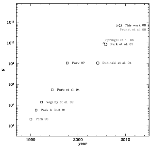
Figure 1 shows how our simulation compares with other recent large simulations in terms of number of particles: the Millennium Run with 10 billion particles, and the recent French collaboration N-body simulation (Teyssier et al. 2008) using 68.7 billion particles. Our Horizon Run contains 69.9 billion particles. The French simulation size was 2000 Mpc while that of the Millennium run was Mpc. Figure 2 shows the sizes of these notable simulations to scale for comparison.
3. The Horizon Run
Here we describe our Horizon Run N-body Simulation. We adopt the CDM model of the universe with the WMAP 5 year parameters listed in Table 1. The initial conditions are generated on a mesh with pixel size of Mpc. The size of the simulation cube is Mpc on a side, and Mpc diagonally. Note that the horizon distance is Mpc. We use billion CDM particles whose initial positions are perturbed from their uniform distribution to represent the initial density field at the redshift of . They are subsequently gravitationally evolved using a TreePM code (Dubinski et al. 2004; Park et al. 2005) with a force resolution of kpc, making 400 global time steps taking about 25 days on the TACHYON111http://www.ksc.re.kr/eng/resources/resources1.htm, a SUN Blade system, at KISTI Supercomputing Center in Korea. It is a Beowulf system with 188 nodes each of which has 16 CPU cores and 32 Gbytes memory. The simulation used 2.4 TBytes of memory, 20 TBytes of hard disk, and 1648 CPU cores. We saved the whole cube data at redshifts , and 1. We also saved the positions of the simulation particles in a slice of constant thickness of Mpc as they appear in the past light cone. In order to make the mock SDSS-III LRG surveys we place observers at 8 locations in the simulation cube, and carry out whole sky surveys up to . These are all past light cone data. The effects of our choices of the starting redshift, time step, and force resolution are discussed in Appendix A, where we use the Zel’dovich redshifts and FoF halo multiplicity function to estimate the effects.
During the simulation we located 8 equally-spaced (maximally-separated) observers in the simulation cube, and saved the positions and velocities of particles at as they cross the past light cone. The subhalos are then found in the past light cone data, and used to simulate the SDSS-III LRG survey. We assume that the SDSS-III survey will produce a volume-limited LRG sample with constant number density of . In our simulation we vary the minimum mass limit of subhalos to match the number density of selected subhalos (the mock LRGs) with this number at each redshift. For example, the mass limit yielding LRG number density of was found to be and at and 0.6, respectively.
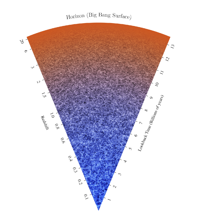
Our larger volume allows us to much better model the true power at large scales, particularly in the case of the LRG distribution, which is critical to the baryon oscillation test. Figure 3 is a Mpc-thick slice through this simulation showing the matter density field in the past light cone all the way to horizon. The thickness of the wedge is constant and the opening angle is 45 degrees. The Earth (the observation point) is at the vertex and the upper boundary is the Big Bang surface at . The distribution of the CDM particles is converted to a density field using the variable-size spline kernel containing 5 CDM particles, and the density field before was obtained by linearly evolving the initial density field backward in time. The radial scale of the slice is the look-back time, so the upper edge corresponds to the age of the universe, 13.6 billion years located at the comoving distance of 10,500Mpc.
4. Modelling of the Luminous Red Galaxies
We use a subhalo finding technique developed by Kim & Park (2006; see also Kim, Park, & Choi 2008) to identify physically self-bound (PSB) Dark Matter subhalos (not tidally disrupted by larger structures) at the desired epoch and identify the most massive ones with LRG galaxies. This does not throw away information on the subhalos which is actually in the N-body simulations and would be thrown away in a Halo Occupation Distribution analysis using just simple friend-of-friend (FoF) halos, and importantly allows us to identify the LRG galaxies without free fitting parameters. We have a mass resolution high enough to model the formation of LRGs whose dark halos are more massive than about (total mass of 30 particles). Within the whole simulation cube we detect 127,890,474 and 92,043,641 subhalos at and 0.5, respectively. The mean separation of these massive subhalos is Mpc at .
Before we proceed with analyzing the mock LRG sample, it will be interesting to see how well it reproduces the physical properties of the existing LRG sample. Kim et al. (2008) and Gott et al. (2008) has shown that the spatial distribution of the subhalos identified in the CDM simulation is consistent with the galaxies in the SDSS Main Galaxy DR4plus sample (Choi et al. 2007). The observed genus, the distribution of local density, and morphology-dependent luminosity function were successfully reproduced by subhalos that are ranked according to their mass to match the number density of galaxies. Moreover, the subhalos identified as LRGs are also shown to reproduce the genus topology of SDSS LRG galaxies remarkably well (Gott et al. 2009). In Appendix B we present a comparison between the correlation functions (CF) of the SDSS LRGs and simulated mock LRGs to examine how accurately our mock LRG galaxies model the observed ones in terms of the two-point statistic. We find a reasonable match between them over the scales from to 140Mpc, particularly in the case of the shape of the CF. Based on our previous and present studies, we conclude that the observed BAO scale and large-scale topology, which this work is focusing on, can be very accurately calibrated using the mock galaxies identified from our gravity-only simulation. One of the reasons is that both are determined by the shape and not by the amplitude of the power spectrum.
It is interesting to know the fraction of mock LRGs that are central or satellite subhalos within FoF halos. This can be a test of consistency with other prescriptions for modeling LRGs (see Zheng et al. 2008 for the Halo Occupation Distribution modeling). For comparison with the SDSS LRG sample (; Zehavi et al. 2005), we build 24 mock LRG samples from eight all-sky past light cone data with the same observation mask of the SDSS survey. Because the LRGs brighter than are extremely rare (Zheng et al. 2008), we do not apply the upper-mass limit to the mock samples (refer to Appendix B for detailed descriptions of generating SDSS LRG surveys). In these mock samples, we count the member galaxies belonging to each FoF halo utilzing the fact that our PSB method identifies the subhalos or mock LRGs within the FoF halos. Among the mock LRGs in a FoF halo, we regard the most massive LRG as the central galaxy and the rest of them as satellites. The mass of a host system is obtained by summing up the masses of all member LRGs. We find that the fraction of the mock LRG galaxies that are satellites in FoF halos is %. This satellite fraction is within the observed range of 5.2 % – 6.2 % (Zheng et al. 2008).
5. BAO Bump in
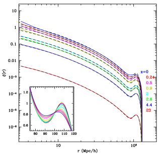
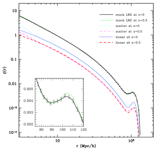
Figure 4 shows the evolution of the CF of the matter density field from to . The dashed curves are the linear CFs, and colored ones are the matter CFs measured at eight redshifts using the whole simulation data. The inset box demonstrates the change in the shape of CF near the baryon oscillation bump due to the non-linear gravitational evolution in the matter field. In the inset box the amplitude of the CF at is scaled so that the peak of the baryon bump has unit amplitude, and then the amplitudes of the CFs at other epoches are scaled to match the CF at at Mpc. The amplitude of the bump decreases by 16%, and the peak location decreases by 4% from the initial epoch to the present.
The top two curves of Figure 5 are the CFs calculated from all mock LRGs in the whole cube at and 0.5. They are also shown in the inset box at the lower left corner. The curve with error bars is the mock LRG CF at . Errors are estimated from sub-cube results. The baryon oscillation bump is clearly visible. Notice the tiny amount of noise, because we are sampling such a large volume. In Figure 5 we also present the 3D covariance function of the matter density field, and linear regime CF at and 0.5 for comparison. The linear theory gives Mpc for the position of the BAO peak while in the mock LRG CFs they are Mpc and Mpc at and 0.5, a difference of up to 3.7 % and 2.7 %, respectively. On the other hand, the matter density field has peak at Mpc and Mpc at these epoches, respectively.
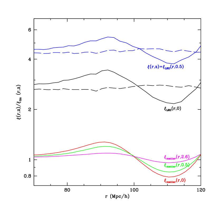
It is important to note that the systematic effects in the baryonic bump in the LRG CF depend on the type of tracer. Because of the high statistical biasing in the distribution of LRGs the evolution of the LRG CF is different from that of the matter CF. In Figure 6 we show the ratio of the matter and mock LRG CFs relative to the linear CF. The bottom three curves are the matter CFs at and 2.6 divided by the linear CF evolved to the corresponding redshifts. The upper two solid curves are the mock LRG CFs at and 0.5 also divided by the linear CF evolved to and 0.5. It can be noted that the deviation from the shape of the linear CF is different in the cases of the matter and mock LRG CFs even though the difference is not large. For example, at the separations of and 70 Mpc the ratio between the LRGs and matter at is about 4.65, but Mpc the ratio is 4.52 a 2.7% difference. The long dashed lines in Figure 6 are the ratios of the mock LRG CF to the evolved matter CF. We can observe small enhancements of the ratio around the baryonic acoustic signature both at and 0.5, and this enhancement is consistent with the results of Desjacques (2008) who used density maxima instead of halos. Therefore, it will be erroneous to use the non-linear matter CF to correct for the observed LRG CF. It is very important to correctly model the LRG galaxies in the -body simulation that have the accurate degree of biasing, and to use them for the correction.

For direct comparison with the Sloan III data, we have made all-sky LRG galaxy surveys using the past light cone data generated at 8 locations in our Horizon Run. The surveys are made so as to maintain the mean number density of LRGs as . Figure 7 shows a fan shaped diagram of a random slice through a mock Sloan III survey.
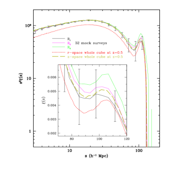
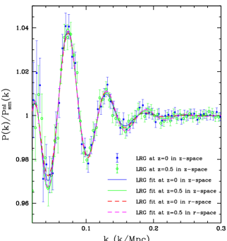
In Figure 8 we present the CFs of the LRGs observed in the mock SDSS-III surveys. At each observer location we make four SDSS-III LRG survey catalogs covering stradian of the sky and extending out to . Each mock LRG sample is then divided into three redshift shells that contain roughly equal number of galaxies. The redshift boundaries between these shells are at and . Three solid lines of Figure 8 are the mean CFs averaged over 32 mock surveys measured in these three shells. We add peculiar velocities along the line-of-sight to simulate the effects of redshift distortion, and measure the covariance function in the past light cone. The error bars for the CF of each redshift shell, obtained from 32 mock surveys, are attached to the CF of the lowest redshift shell (). We observe in the redshift-distorted samples a substantial increase in the CF amplitude on larger scales (), especially on the BAO scale. This shift of the BAO amplitude between redshift slices was also seen in the Fig. 19 of Cabre & Gaztanaga (2009) who used SDSS LRG samples for their analysis. They tried to explain the BAO-amplitude shift by introducing possible systematic effects in the SDSS observation but they did not give any conclusion. However, it is interesting to observe a similar shift in the mock surveys which does not suffer from the systematic effect.
The local peak in the CF measured from individual mock survey data shows a large variation, and so we developed a method that can measure the BAO bump position more accurately. The position of the BAO bump was measured by fitting the observed CF to a set of template CFs. The template CFs are those selected from the simulated matter CFs from to 0. As shown in Figure 4, the matter CF is accurately known, and shows a wide range of variation in the amplitude and shift of the BAO bump. To fit an observed CF to the templates, we calculate
| (1) |
where and are the amplitude and shift parameters. Here we set and to safely include the bump. We numerically find the free parameters and that minimize to determine the best-fit template, and to estimate the position of the BAO bump.
A close inspection reveals that the peak location and amplitude of the BAO bump in the LRG CF slowly decrease as redshift decreases; the location of the BAO bump is at , , and Mpc for , and shells, respectively. Due to the sample variance the uncertainty in the BAO scale amounts as much as 5.0%. For a comparison the real space and redshift space CFs of all LRGs in the simulation box at are also plotted in dotted and dashed curves, respectively. Their BAO bump peaks are located at 105.2 and Mpc, respectively.
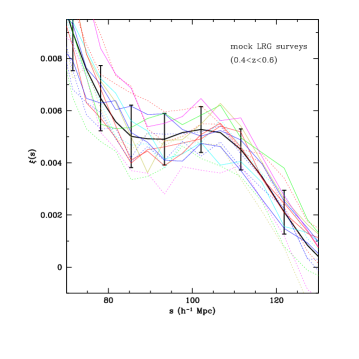
The uncertainty in the BAO bump position can be reduced if larger samples are used. We measure the CF of mock LRG galaxies located in a redshift shell with inner and outer boundaries at and 0.6, respectively. This region contains more data than previous settings leading to smaller scatter around the average (see Fig. 9). The mean value of the BAO peak position over 32 mock surveys is 103.2Mpc and the difference from the linear regime initial conditions is Mpc. Thus if the BAO peak is measured as in our analysis, the peak location should be corrected upward by above value. The uncertainty in this systematic correction is also estimated from our 32 mock SDSS-III surveys. This gives us a benchmark idea of the extent of the systematic effects (and their uncertainty) encountered in measuring the position of the BAO bump from LRGs and comparing it with the baryon oscillation scale from the linear regime theory. As hoped for, the systematic effects due to non-linear effects and biasing are small, and can be corrected for with high accuracy. The corrected value will only be in error by the uncertainty in the correction factor which is 2.5% when the data in this thick shell is used. Comparison of the individual 32 mock Sloan III surveys after such systematic corrections have been made will give us an accurate measure of the statistical accuracy of the results on that we should expect in the real survey.
These preliminary studies can be used to improve the survey strategy and reconstruction methods before the survey starts. In the simulations we are omniscient since we know where each of the LRG galaxies actually originated, so this should help us to design and improve the reconstruction techniques. As the data is being collected, and the selection function of the LRG galaxies being detected becomes accurately known, it will be possible to improve the accuracy of these studies as the survey continues. Comparisons with the N-body simulations should be of critical value, allowing one to calibrate the dark energy experiment with high accuracy.
6. BAO Wiggles in
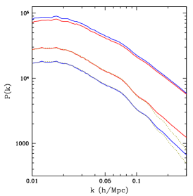
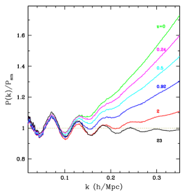
A BAO bump in the correlation has a wiggle pattern in the power spectrum (hereafter PS). Also similar changes, the shift and degrading of shapes, happen to the baryonic wiggles of PS. Recently, Seo et al. (2008) reported that they have detected sub percentage level of shift of the BAO wiggle after applying a fitting to the matter PS. Therefore, it is valuable to check whether LRG galaxies, as a biased peak, have a similar level of shift or they have different scale of shift compared to the matter field. Figure 10 shows the mock LRG power spectra in real (the second top line) and redshift (topmost line) spaces at and matter PS at (bottom line) and 0. Figure 11 shows the evolution of the simulated matter PS normalized by the smoothed PS () around baryonic scales (Eisenstein & Hu 1998). As can be seen, the non-linear gravitational evolution affects the wiggle pattern from small scales making them degraded in shape and buried in nonlinear background with time. Oscillatory features at Mpc experience a severe distortion in shape while the features on the larger scales show less deviations from the linear shapes.
To quantify the non-linear distortion of the BAO feature in the PS of mock LRG galaxies, we followed the analysis of Seo et al. (2008) who introduced the shift () and degrading () parameters in the polynomial fitting functions. The contrast of the baryonic feature is obtained by subtracting the smoothed background PS () of no wiggle form from the linear PS ():
| (2) |
The fitting function is organized as
| (3) |
where reflects the scale-dependent biasing and mode coupling, and is added to account for shot noise. For the -fit, we adopt the polynomial forms:
| (4) |
This functional form provides a reasonable fit to the data and, therefore, we will not consider other alternatives listed in Seo et al. (2008). And is the shifted model PS with a degrading factor:
| (5) |
The linear PS subtracted by the smoothed power is suppressed by a Gaussian damping of length, . Seo et al. (2008) fixed it as Mpc for the matter field at . However, we treat it as a free parameter here because we are dealing with biased subhalos while Seo et al. used the matter particles. The shift parameter, , is added to account for the shift of the baryonic features due to the non-linear evolution and biasing.
In Figure 12 shown are the ratio of the LRG PS to the smoothed non-linear PS (). It shows the contrast of the BAO wiggles over the smooth background PS. The smoothed PS in the non-linear regime is obtained by applying
| (6) |
where we adopt the same values of and as previously obtained when performing the fitting to the simulated power spectrum of the LRG galaxies.
The fitting results are , Mpc, and DOF=0.43 at and, , Mpc, and DOF=0.47 at for LRG galaxies in redshift space. For the real-space data, is unchanged while decreases slightly. The negative value of means that the baryonic feature of the LRG galaxies is moving toward small scales relative to the linear PS. We detected a 2% wiggle shift for the LRG galaxies while Seo et al. (2008) found 0.45% at for the matter field. This significantly larger shift is mainly due to the biasing effect and should be kept in mind when interpreting the observational data to recover the oscillation scales in the PS. Also the degrading parameter (Mpc) is larger than Mpc at which was adopted for matter field by Seo et al. (2008). The more negative shift and larger degrading parameter for the mock LRG galaxies relative to the background matter density field, again demonstrate the tracer dependence of the non-linear effects. We have also applied above analysis to the matter field in real space. The value of is , and 0 at , 0.5, 2, and 23, respectively. Also we obtain , 6.60, 3.75, and 0 Mpc for each redshift. These results are consistent with Seo et al. (2008).
7. Genus Topology of Large Scale Distribution of LRG Galaxies
Through the genus topology analysis one can check whether or not the mock LRG galaxies in our simulation correctly reproduce the spatial distribution of the observed LRGs. At scales larger than the correlation length the LRG genus curve is well-approximated by the Gaussian random phase curve with expected small shifts due to non-linear effects and biasing.
We have developed tools for analyzing the genus topology of large scale structure in the universe (Gott, Dickinson, & Melott 1986; Hamilton, Gott, & Weinberg 1986; Gott, Weinberg, & Melott 1987; Gott, et. al. 1989; Vogeley, et. al. 1994; Park, Kim, & Gott 2005; Park et. al. 2005). We smooth the spatial distribution of galaxies to construct density contour surfaces. We measure the genus as a function of density, allowing comparison with the topology expected for Gaussian random phase initial conditions, as predicted in a standard big bang inflationary model (Guth 1981; Linde 1983) where structure originates from random quantum fluctuations in the early universe. We smooth the galaxy distribution with a Gaussian smoothing ball of radius , where is chosen to be greater than or equal to the correlation length to reduce the effects of non-linearity, and greater than or equal to the mean particle separation to reduce the shot noise effects.
Density contour surfaces are labeled by , where the volume fraction on the high density side of the density contour surface is :
| (7) |
The genus curve is given by the topology of the density contour surface:
| (8) |
(Gott et al. 1986). An isolated cluster has a genus of by this definition. Since is equal to minus the integral of the Gaussian curvature over the area of the contour surface divided by , we can measure the genus with a computer program (CONTOUR3D) (see Gott et al. 1986, 1987). For Gaussian random phase initial conditions:
| (9) |
where and is the average value of integrated over the smoothed power spectrum (Hamilton et al. 1986; Adler 1981; Doroshkevich 1970; Gott et al. 1987). The % median density contour () shows a predicted sponge-like topology (holes), the % high density contour () shows isolated clusters while the % density contour () shows isolated voids.
When the smoothing length is much greater than the correlation length, fluctuations are still in the linear regime and since fluctuations in the linear regime grow in place without changing topology, the topology we measure now should reflect that of the initial conditions, which should be Gaussian random phase according to the theory of inflation (Gott et al. 1987; Melott 1987). Small deviations from the random phase curve give important information about biased galaxy formation and non-linear gravitational effects as shown by perturbation theories and large N-body simulations (c.f. Matsubara 1994; Park et al. 2005). All previous studies have shown a sponge-like median density contour as expected from inflation (Gott et al. 1986, 1989, 2009; Moore et al. 1992; Vogeley et al. 1994; Canavezes et al. 1998; Hikage et al. 2002, 2003; Park et al. 2005)
Small deviations from the Gaussian random phase distribution are expected because of non-linear gravitational evolution and biased galaxy formation and these can now be observed with sufficient accuracy to do model testing of galaxy formation scenarios.
The genus curve can be parameterized by several variables. The amplitude of the genus curve, proportional to of the smoothed power spectrum, gives information about the power spectrum and on the phase correlation of the density distribution. Shifts and deviations in the genus curve from the overall theoretical random phase case can be quantified by the following variables:
| (10) |
| (11) | |||||
| (12) |
where is the genus of the random phase curve (Eq. 8) best fit to the data. Thus, measures any shift in the central portion of the genus curve. The theoretical curve (Eq. 8) has . A negative value of is called a “meatball shift” caused by a greater prominence of isolated connected high-density structures which push the genus curve to the left. This can be due to non-linear galaxy clustering and bias associated with galaxy formation. (and ) measure the observed number of voids (and clusters), respectively, relative to those expected from the best fitting theoretical curve.
Park et al. (2005) show that can result from biasing in galaxy formation because voids are very empty and can coalesce into a few larger voids. A value of can occur because of non-linear clustering, when clusters collide and merge, and if there is a single large connected structure like the Sloan Great Wall. As Park et al. (2005) have shown, with Matsubara’s (1994) formula for second-order gravitational non-linear effects alone, one has the result that at all scales, so if we observe both and to be less than 1, for example, biased galaxy formation must be involved.
Gott et al. (2009) compared observational genus curves from the SDSS survey with a few recent -body simulations. The semi-analytic model of galaxy assignment scheme applied to the Millennium run (Springel et al 2005) gives reasonable values for and , but its value of differs from the observational data by 2.5 , showing less of a “meatball” shift than the data. This indicates a need for an improvement in either its initial conditions (it used a bias factor that is too low according to WMAP 5 year results) or its galaxy formation algorithm (Gott et al. 2008).
Gott et al. (2009) recently measured the 3D topology of the LRG galaxies from the Sloan Survey and measured small deviations from the Gaussian form using , and from Equation 10 to 12. There is only a small amount of noise in the genus curve due to the large sample size. The results are compared with the genus curves averaged over twelve mock LRG galaxy surveys that are performed in a particle CDM simulation (Gott et al. 2009). The mean of the mock surveys fits the observations extraordinarily well, including the fact that the number of voids, as measured by the depth of the valley at or by , is less than the number of clusters, as measured by the depth of the valley at or by , which is also seen in the observations. The fact that the clusters outnumber the voids is due to non-linear biasing and gravitational evolution effects, and they are modeled by the simulations very well. The observed amplitude of the genus curve at and Mpc scales agrees extremely well with the mean of the mock N-body catalog. This indicates that the shape of power spectrum is also modeled extremely well. The observed values of , and are within approximately of those expected from the 12 mock catalogs, all without any free fitting parameters (see Gott et al. 2009 for details). This suggests that finding the LRGs is a clean problem, which can be calculated using CDM particles and gravity. The genus topology is an important check that the N-body simulations here are doing a good job identifying the LRG galaxies.
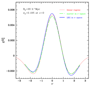
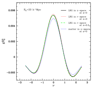
We now present the genus topology analysis of the Horizon Run. Figure 13 compares the genus curves of the matter density field (dashed line) and mock LRG distribution (thick solid line) calculated from the whole simulation cube using the periodic boundary condition. The distribution of our mock LRG galaxies in the simulation cube is smoothed with a smoothing length of Mpc. The curves are compared with the random phase Gaussian curve (thin solid line from to 3.3) corresponding to the CDM model we adopted (see Eq. 9). Note that the LRG genus curve shows more deviations in the high-density regions () from the Gaussian curve than the matter genus curve. This is because the mock LRGs are biased objects, so we see more of them in the crowded regions relative to the background matter. The overall amplitude of the LRG genus curve is very close to that of the linear one.
In Figure 14 we show the mock LRG genus curves for the entire cube in real (thin sold line) and redshift space (thick solid line) at redshift . The redshift space distortion is mimicked by adding the -component of peculiar velocities of mock LRGs to their positions. The smoothing scale is again Mpc. The dotted line is the matter genus curve in redshift space. It can be seen that the redshift space distortion effects make the amplitude of the genus curve decrease. But the genus curve of mock LRGs is much less affected by the redshift distortion when compared with that of matter field. This is again due to the strong statistical biasing of the LRG galaxies. These curves are compared with the genus curve of mock LRG galaxies in real space at redshift (dashed line).
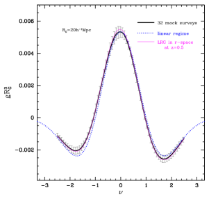
Figure 15 shows the mean genus curves averaged over 32 mock SDSS-III LRG surveys. Each survey is a cone-shaped volume extending out to redshift along the past light cone of our Horizon Run, and the whole survey cone is used to calculated the genus curve. Peculiar velocities are added to radial distances of LRGs to mimic the redshift distortion effects. Since the mock LRGs have the mean density of or a mean separation of 15Mpc, the smoothing length of Mpc is large enough to beat down the shot noise effects. Also shown are the real space genus curves of the mock LRGs at redshift and of the random phase Gaussian density field corresponding to the CDM model adopted in our simulation. Note that there is no fitting involved. The error bars are obtained from the genus distribution of 32 mock LRG surveys.
The genus curves of mock LRGs deviate from the linear regime curve because of non-linear biasing and gravitational effects. Table 2 lists the genus-related parameters at the Gaussian smoothing scale of Mpc for LRGs measured from the whole simulation cube and from the 32 mock SDSS-III surveys. For the whole simulation cube results (the second and third columns) the error bars are estimated based on the variance in these parameters seen in 64 quarter-sized subsamples. For mock SDSS-III LRG survey results the estimates are the mean values averaged over 32 mock SDSS-III surveys, and the error bars are for a single survey. The linear regime predictions are also given for comparison.
| Parameters | Real Space | Redshift Space | Mock SDSS-III | Linear Regime Prediction |
|---|---|---|---|---|
| 0 | ||||
| 1 | ||||
| 1 |
Note. — Cols. (1) Genus parameter (2) Mock LRGs in real space at (3) Mock LRGs in redshift space at (4) Mock LRGs in past light-cone space (5) Linear regime predictions
It can be seen that the amplitude of the observed genus curve of the mock SDSS-III LRGs is only 0.6% different from that of the linear theory expectation, and will be determined with 1.5% uncertainty. The non-Gaussian parameters and show statistically significant deviations from the Gaussian curve, which is characteristic of the LRGs identified in our simulation.
8. Conclusions
Baryon oscillations are believed to be the method of characterizing dark energy “least affected by systematic uncertainties” according to the Dark Energy Task Force Report. But the baryon oscillation is affected by all kinds of non-linear effects, so comparison with large N-body simulations is essential to control the systematics. Gott et al. (2009)’s study of the topology of the LRG galaxy clustering in the current SDSS shows that large N-body simulations are accurately modeling these non-linear gravitational and biased galaxy formation effects.
To aid in calibrating non-linear gravitational and biasing effects in the future Sloan-III baryon oscillation scale survey (BOSS), we have made here a large N-body simulation: billion particles in a Mpc box, which models the formation of LRGs in this region. Using improved values over those adopted by the Millennium Run, which was based on WMAP-1 initial conditions (Spergel et al. 2003), our simulation has more power at large scales ( versus , which should make for a higher frequency of large scale structures), and more accurate normalization at Mpc scale ( while Millennium Run used ).
We have made 32 mock surveys of the Sloan III survey, which should allow us to correct for small systematic effects in the measurement of the physical scale of the baryon oscillation peak as a function of redshift. We predict from our mock surveys that the BAO peak scale can be measured with the cosmic variance-dominated uncertainty of about 5% when the SDSS-III sample is divided into three equal volume shells, or about 2.6% when a thicker shell with is used. We find that one needs to correct the scale for the systematic effects amounting up to 5.2% to use it to constrain the linear theories.
The amplitude of the genus curve measured in redshift space in the mock SDSS III survey is, in the mean, expected to be equal to the linear regime prediction to an accuracy of about 2% at the smoothing scale of 20 Mpc. So the systematic evolution correction in the amplitude of the genus curve will be tiny. Also, the RMS uncertainty in the amplitude in the genus curve due to the cosmic variace as measured in one SDSS-III survey is only 1.5% at 20 Mpc scale. Since the uncertainty scales with inverse square root of the number of resolution elements (or equivalently with ), this implies the uncertainty of about 1.0% at 15 Mpc scale, which will be the mean separation of the SDSS-III LRGs. In subsequent papers we shall show how measuring the amplitude of the genus curve at different smoothing length makes possible an independent measure of scale complimenting the baryonic oscillation bump method for measuring .
As dark energy makes up three quarters of the universe today, making such improvements in characterizing dark energy are particularly exciting. Much ancillary science can be done with this large N-body simulation; detailed modeling of the integrated Sachs-Wolf effect and comparison with counts of LRG galaxies in the sky, for example. We can search for Great Walls and voids to estimate their frequency and size (Gott et al. 2005). Here, our large volume size and WMAP-5 based initial conditions (Komatsu et al. 2008) should be of great benefit. We will make the simulation data available to the community (See http://astro.kias.re.kr/Horizon-Run/ for information). Please cite this paper when the simulation data is used.
Appendix A A. The Starting Redshift and the number of time steps
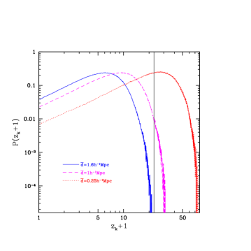
The TreePM code (Dubinski et al. 2004) used in this paper adopts the first-order Lagrangian perturbation scheme to generate the initial Zel’dovich displacement (for comparison with the second-order scheme, refer to Crocce et al. 2006 and references therein). The starting redshift of the simulation should be chosen so that the Lagrangian shifts of particles are not larger than the pixel spacing. This is because, if the initial displacement is larger than a pixel spacing, a particle may not fully experience the local differential gravitational potential (or Zel’dovich force) and, consequently, the shift calculated by using the first-order scheme could not fully reflect the fluctuations at the pixel scale. To quantitatively estimate the proper starting redshift, we introduce the Zel’dovich redshift, , of a particle defined as the epoch when its Zel’dovich displacement becomes equal to the pixel size either in , , or direction. In Figure 16, we show the distribution function of the Zel’dovich redshift, , for three simulations tagged by the mean particle separation (), or equivalently the pixel size. To measure the distribution, we perform an initial setting moving particles from the initial conditions defined on a -size mesh. One should acknowledge a lack of the large-scale power causing a possible underestimation of especially for the small simulation. Each distribution shows a power-law increase with and a sharp drop after a peak. It can be seen that no particle experiences a shift larger than a pixel size at when Mpc, which justifies our choice of the initial redshift.
We adopted 400 time steps to evolve the Cold Dark Matter particles from to 0. We set the force resolution to 0.1 . Here we present a test justifying our choice of the number of time steps.
Due to this relatively larger step size and lower force resolution, one may raise a question about the simulation accuracy whether it may have sufficient time and force resolutions to correctly model the formation of halos and subhalos.
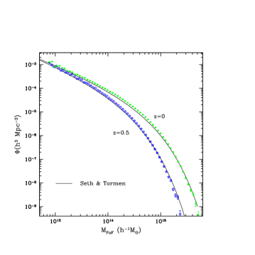
One of the simplest ways to judge whether a simulation retains a sufficient power to resolve small structures is to compare the simulated FoF halo mass function with the well-known functions obtained from very high resolution simulations with a special emphasis on the population of less massive halos. This is because coarse time-step size or poor force resolution may destroy smaller structures more easily. In Figure A2, Sheth & Tormen (1999; dotted)’s fitting function is shown at (upper) and 0.5 (lower). The corresponding FoF halo mass functions from our simulation are shown by filled squares () and open circles (). This comparison demonstrates that the Horizon Run resolves structures with mass down to about (, which is the mass of 30 simulation particles. This mass limit is below the expected lower mass limit of the BOSS LRGs, and therefore formation of the dark halos associated with the BOSS LRGs are accurately simulated by the Horizon Run.
Appendix B B. Correlation Functions of Mock and SDSS LRG Galaxies
To compare the CFs of the SDSS LRG and simulated mock LRG samples we built 24 mock SDSS LRG samples from eight all-sky past light cone data in a way that they do not overlap with one another. We apply the same mask of the SDSS survey (i.e. the SDSS-I plus SDSS-II). We use the SDSS LRG sample (S1; , ) which is described in detail by Gott et al. (2009). Here, is the absolute magnitude measured at (We omit the subscript 0.3 in Figure B1). We re-calculate the comoving distance based on the WMAP 5-year cosmology and obtain the mean number density of the LRGs as which is slightly lower than the previous measurement, obtained by using the WMAP 3-year parameters. As the number density of LRGs in the sample S1 is nearly constant over redshift (Zehavi et al. 2005), the lower-mass limit of the corresponding mock LRGs (dark halos) should be a function of redshift. We apply the redshift-invariant multiplicity function of subhalos (or LRGs) to find the relation between the critical mass and redshift. This method allows a small fluctuation across 24 surveys in the mean number density of mock galaxies (). Also we apply the redshift distortions to the mock galaxies to mimick observations.
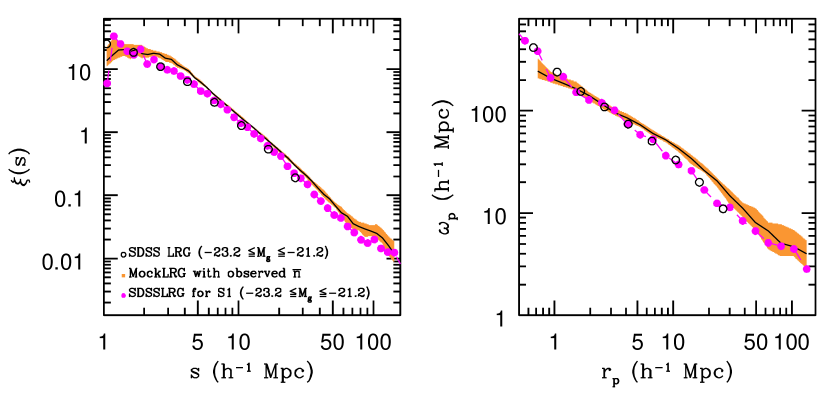
The left panel of Figure 18 shows the average CF of mock LRGs (solid line) together with the 1– limits (shaded region) measured on the past light cone surface. Open circles are the CF of the SDSS LRGs calculated by Zehavi et al. (2005) based on the spatially-flat cosmology and filled circles are the CF measured by us using the SDSS LRG data (S1) based on the WMAP 5-year cosmology. The error bars of the observational data should be similar to those of the mock survey data. The simulated LRG sample has a CF that impressively mimics the observations both in shape and amplitude. But its amplitude seems slightly higher than that of the observation by 5% – 15% on the intermediate scales ().
The projected CF, , is another measure of the consistency between simulation and observation. The projected distance () and the radial distance () between two LRGs is related to each other by where is the three-dimensional distance between the pair in redshift space. The projected correlation is obtained by integrating the two-dimensional CF along the line of sight:
| (B1) |
where corresponds to the survey depth in the radial direction. In the right panel of Figure 18, we show the mean (solid line) and the 1– limit (shaded region) of the projected CFs measured from the 24 simulated LRG samples. These simulated CFs match the observed counterparts well except that it is slightly higher at , which was also seen in the three-dimensional CF. This deserves further analysis and will be investigated in a separate paper.
References
- Aarseth et al. (1979) Aarseth, S.J., Gott, J.R., & Turner, E.L. 1979, ApJ, 228, 664
- Abell et al. (1989) Abell G. O., Corwin H. G., & Olowin R. P., 1989, ApJS, 70, 1
- Adler (1981) Adler, R.J. 1981 The Geometry of Random Fields, Chichester, Wiley
- Albrecht et al. (2006) Albrecht, A., Bernstein, G., Cahn, R., Freedman, W.L., Hewitt, J., Hu, W., Huth, J., Kamionkowski, M., Kolb, E.W., Knox, L., Mather, J.C., Staggs, S., Suntzeff, N.B. 2006, astro-ph/0609591
- Bertschinger (1985) Bertschinger, E. 1985, ApJS, 58, 1
- Bhavsar et al. (1981) Bhavsar, S.P., Aarseth, S.J., & Gott, J.R. 1981, ApJ, 246, 656
- Canavezes et al (1998) Canavezes, A., et al. 1998, MNRAS, 297, 777
- Cabre & Gaztanaga (2009) Cabre, A. & Gaztanaga, E. 2009, MNRAS, 393, 1183
- (9) Choi, Y.-Y., Park, C., & Vogeley, M. S. 2007, ApJ, 658, 884
- Colberg et al. (2000) Colberg, J.M., White, S.D M., Yoshida, N., MacFarland, T.J., Jenkins, A., Frenk, C.S., Pearce, F.R., Evrard, A.E., Couchman, H.M.P., Efstathiou, G., Peacock, J.A., Thomas, P.A., and The Virgo Consortium 2000, MNRAS, 319, 209
- Crocce et al. (2006) Crocce, M., Pueblas, S., & Scoccimarro, R. 2006, MNRAS, 373, 369
- Crocce & Scoccimarro (2008) Crocce, M. & Scoccimarro, R. 2008, PRD, 77, 3533
- Crotts et al. (2005) Crotts, A., Garnavich, P., Priedhorsky, W., Habib, S., Heitmann, K., Wang, Y., Baron, E., Branch, D., Moseley, H., Kutyrev, A., Blake, C., Cheng, E., Dell’Antonio, I., Mackenty, J., Squires, G., Tegmark, M., Wheeler, C., & Wright, N., 2005, astro-ph/0507043
- Desjacques (2008) Desjacques, V. 2008, PRD, 78, 103530
- Doroshkevich (1970) Doroshkevich, A.G. 1970, Astrophysics, 6, 320
- Dubinski et al. (2004) Dubinski, J., Kim, J., Park, C., & Humble, R. 2004, New Astronomy, 9, 111
- Eisenstein et al. (2007a) Eisenstein, D. J., Seo, H.-J., & White, M. 2007, ApJ, 664, 660
- Eisenstein et al. (2007b) Eisenstein, D. J., Seo, H.-J., Sirko, E., & Spergel, D.N. 2007, ApJ, 664, 675
- Eisenstein et al. (2001) Eisenstein, et al. 2001, AJ, 122, 2267
- Eisenstein & Hu (1998) Eisenstein, D. J. & Hu, W. 1998, ApJ, 496, 605
- Fillmore & Goldreich (1984) Fillmore, J.A. & Goldreich, P. 1984, 281, 9
- Geller & Huchra (1989) Geller, M.J. & Huchra, J.P. 1989, Science, 246, 897
- Groth & Peebles (1975) Groth, E.J. & Peebles, P.J.E. 1975, BBAS, 7, 425
- Gott et al. (2009) Gott, J.R., Choi, Y.-Y., Park, C., & Kim, J. 2009, ApJ, 695, L45
- Gott et al. (1986) Gott, J.R., Dickinson, M., & Melott, A.L. 1986, ApJ, 306, 341
- Gott et al. (2008) Gott, J.R., Hambrick, D.C., Vogeley, M.S., Kim, J., Park, C., Choi, Y.-Y., Cen, R., Ostriker, J.P., & Nagamine, K. 2008, ApJ, 675, 16
- Gott et al. (1989) Gott, J.R., Miller, J., Thuan, T.X., Schneider, S.E., Weinberg, D.H., Gammie, C., Polk, K., Vogeley, M., Jeffrey, S., Bhavsar, S.P., Melott, A.L, Giovanelli, R., Hayes, M.P., Tully, R.B., & Hamilton, A.J. 1989, ApJ, 340, 625
- Gott & Rees (1975) Gott, J.R. & Rees, M.J. 1975, å, 45, 365
- Gott & Turner (1977) Gott, J.R. & Turner, E.L. 1977, ApJ, 216, 357
- Gott et al. (1979) Gott, J.R., Turner, E.L., & Aarseth, S.J. 1979, ApJ, 234, 13
- Gott et al. (1987) Gott, J.R., Weinberg, D., & Melott, A.L. 1987, ApJ, 319, 1
- Gunn & Gott (1972) Gunn, J.E. & Gott, J.R. 1972, ApJ, 176, 1
- Guth (1981) Guth, A.H. 1981, PRD, 23, 347
- Hamilton et al. (1986) Hamilton, A.J.S., Gott, J.R., & Weinberg, D. 1986, ApJ, 309, 1
- Hikage (02) Hikage, C. et al. 2002, PASJ, 54, 707
- Hikage (03) Hikage, C. et al. 2003, PASJ, 55, 911
- Hockney & Eastwood (1981) Hockney, R. W., & Eastwood, J. W. 1981, Computer Simulations Using Particles, McGraw-Hill, New York Colberg, J.M., White, S.D.M., Couchman,H.M.P., Peacock, J.A., Efstathiou, G., & Nelson, A.H. 1998 ApJ, 499, 20
- Kim & Park (2006) Kim, J. & Park, C. 2006, ApJ, 639 600
- Kim et al. (2008) Kim, J., Park, C. & Choi, Y.-Y. 2008, ApJ, 683 123
- Linde (1983) Linde, A.D. 1983, Physics Letter B, 129, 177L
- Lukic et al. (2007) Lukic, Z., Heitmann, K., Habib, S., Bashinsky, S., & Ricker, P. M. 2007, ApJ, 671, 1160
- Matsubara (1994) Matsubara, T. 1994, ApJ, 434, 43
- Melott (1987) Melott, A.L. 1987, MNRAS, 228, 1001
- Miller et al. (2005) Miller, et al. 2005, ApJ, 130, 968
- Moore et al. (1992) Moore, B., Frenk, C.S., Weinberg, D.H., Saunders, W., Lawrence, A., Ellis, R.S., Kaiser, N., Efstathiou, G., & Rowan-Robinson, M. 1992, MNRAS, 256, 477
- Park (1990) Park, C. 1990, MNRAS, 242, 59
- Park et al. (2005a) Park, C., Kim, J., & Gott, J.R. 2005, ApJ, 633, 1
- Park et al. (2005b) Park, C., Choi, Y.-Y., Vogeley, M.S., Gott, J.R., Kim, J., Hikage, C., Matsubara, T., Park, M.-G., Suto, Y., & Weinberg, D.H. 2005, ApJ, 633, 11
- Peebles (1970) Peebles, P.J.E. 1970, AJ, 75, 13
- Percival et al. (2007) Percival, W.J., Cole, S., Eisenstein, D.J., Nichol, R.C., Peacock, J.A., Pope, A.C., Szalay, A.S. 2007, MNRAS, 381, 1053
- Press & Schechter (1974) Press, W. H. & Schechter, P. 1974, ApJ, 187, 425
- Seo & Eisenstein (2005) Seo, H.-J. & Eisenstein, D.J. 2005, ApJ, 633, 575
- Seo et al. (2008) Seo, H.J., Siegel, E.R., Eisenstein, D.J., & White, M. 2008, arXiv:0805.01117
- Sheth & Tormen (1999) Sheth, R. K. & Tormen, G. 1999, MNRAS, 308, 119
- Spergel et al. (2003) Spergel, et al. 2003, ApJS, 148, 175
- Spergel et al. (2006) Spergel. D.N., Bean, R., Dore, O., Nolta, M.R., Bennett, C.L., Dunkley, J., Hinshaw, G., Jarosik, N., Kormatsu, E., Page, L., Peiris, H.V., Verde, L., Halpern, M., Hill, R.S., Kogut, A., Limon, M., Meyer, S.S., Odegard, N., Tucker, G.S., Weiland, J.L., Wollack, E., & Wright, E.L. 2007, ApJS, 170, 377
- Springel et al. (2005) Springel, V., White, S.D.M., Jenkins, A., Frenk, C.S., Yoshida, N., Gao, L., Navarro, J., Thacker, R., Cronton, D., Helly, J., Peacock, J.A., Cole, S., Thomas, P., Couchman, H., Evrard, A., Colberg, J., & Pearce, F. 2005, Nature, 435, 629
- Teyssier et al. (2008) Teyssier, R., Pires, S., Prunet, S., Aubert, D., Pichon, C., Amara, A., Benabed, K., Colombi, S., Refregier, A., & Starck, J. 2008, arXiv:0807.3651, submitted to A&A
- Vogeley et al. (1994) Vogeley, M.S., Park, C., Geller, M.J., Huchra, J.P., & Gott, J.R. 1994, ApJ, 420, 525
- Warren et al. (2006) Warren, M. S., Abazajian, K., Holz, D. E., & Teodoro, L. 2006, ApJ, 646, 881
- Zehavi et al. (2005) Zehavi, et al. 2005, 621, 22
- Zheng et al. (2008) Zheng, Z., Zehavi, I., Eisenstein, D. J., Weinberg, D. H., Jin, Y. 2008, arXiv:0809.1868v1