Experimental study of out of equilibrium fluctuations in a colloidal suspension of Laponite using optical traps

Abstract

This work is devoted to the study of displacement fluctuations of micron-sized particles in an aging colloidal glass. We address the issue of the validity of the fluctuation dissipation theorem (FDT) and the time evolution of viscoelastic properties during aging of aqueous suspensions of a clay (Laponite RG) in a colloidal glass phase. Given the conflicting results reported in the literature for different experimental techniques, our goal is to check and reconcile them using simultaneously passive and active microrheology techniques. For this purpose we measure the thermal fluctuations of micro-sized brownian particles immersed in the colloidal glass and trapped by optical tweezers. We find that both microrheology techniques lead to compatible results even at low frequencies and no violation of FDT is observed. Several interesting features concerning the statistical properties and the long time correlations of the particles are observed during the transition.

1 Introduction

The description of out-of-equilibrium systems is a topic of major interest in physics since in most systems, energy or matter flows are not negligible but drive them into non-ergodic states for which equilibrium statistical mechanics may be not applicable. The typical examples of such systems are slowly stirred systems and glasses. Unlike equilibrium statistical mechanics, whose foundations are well established since long time ago, non-equilibrium statistical mechanics is still being developed.

One attempt to develop a statistical mechanics description of non-equilibrium slowly evolving systems is to extend some equilibrium concepts to them, namely the so called fluctuation dissipation theorem (FDT). FDT relates the power spectral density of equilibrium fluctuations of a given observable $x$ of systems in contact with a thermal bath at temperature $T$ to the response $\chi$ to a weak external perturbation. In frequency domain the relation between the corresponding Fourier transforms involves a prefactor given by $T$

$$\langle|\hat{x}(\omega)|^{2}\rangle=\frac{4k_{B}T}{\omega}Im\{\hat{\chi}(\omega)\}.$$ (1)

Despite of the fact that a thermodynamic temperature is not rigorously defined for non-equilibrium systems, a generalization of FDT can be done by means of an effective temperature $T_{eff}(\omega,t_{w})$ which describes fluctuations at a time scale $1/\omega$. It is defined as :

$$T_{eff}(\omega,t_{w})=\frac{\omega\langle|\hat{x}(\omega,t_{w})|^{2}\rangle}{4k_{B}Im\{\hat{\chi}(\omega,t_{w})\}},$$ (2)

where $t_{w}$ denotes the age of the system, i.e. the waiting time since the systems left equilibrium. In general, for a non-equilibrium system either the spectral density of fluctuations and the response function depend on $t_{w}$ and then violations of FDT ($T_{eff}(\omega,t_{w})\neq T$) could also depend on it.

Glasses are one of the examples of non-equilibrium systems that have been studied extensively over the past years. They are disordered systems at microscopic length scales formed after a quench from an ergodic phase (e.g. an ordinary liquid in equilibrium) to a non-ergodic phase (e.g. a supercooled liquid). After a quench, a glassy system relaxes asymptotically to a new phase in equilibrium with the new temperature $T$ of its surroundings, but the time needed to reach equilibrium may be extremely large. Since the system is non-ergodic during its relaxation, there is no invariance under time translations and then its age $t_{w}$ is well defined. The slow time evolution of their physical properties (e.g. viscosity) is known as aging. A number of theoretical, numerical and experimental studies have shown that two different effective temperatures are found for structural glasses [3], [4] and spin glasses [5], [6], [7]. One of them is the effective temperature associated to the fast rattling fluctuations (high frequency modes) and is equal to $T$. The other effective temperature is the one associated to the slowest structural rearrangements (low frequency modes) whose value is larger than $T$ and decreases with time to $T$. Both effective temperatures have the properties of thermodynamic temperatures in the sense that they correspond to two different thermalization processes at different time scales [8].

1.1 FDT in Laponite suspensions

Regarding the existence of an effective temperature higher than the bath temperature for structural and spin glasses, several recent works have attempted to look for violations of FDT in another kind of non-equilibrium systems: colloidal glasses. Unlike structural or spin glasses, the formation of either a colloidal glass or a gel [9] does not require a temperature quench but the packing of colloidal particles at a certain low concentration in water forming a glassy structure.

Aqueous suspensions of clay Laponite have been studied as a prototype of colloidal glasses. Laponite is a synthetic clay formed by electrostatically charged disc-shaped particles of chemical formula Na${}^{+}_{0.7}$[Si₈Mg_5.5Li_0.3O₂₀(OH)₄]^0.7- whose dimensions are 1 nm (width) and 25 nm (diameter). When Laponite powder is mixed in water, the resulting suspension undergoes a sol-gel transition in a finite time (e.g. a few hours for 3 wt %), i.e. it turns from a viscous liquid phase (sol) into a viscoelastic solid-like phase (gel). During this aging process, because of electrostatic attraction and repulsion, Laponite particles form a house of cards-like structure.

Several properties of Laponite suspensions during aging have been extensively studied, such as viscoelasticity [10], translational and rotational diffusion [11] and optical susceptibility [12] using techniques such as rheology and dynamic light scattering. However, the available results obtained so far for the issue of the validity of the FDT in this system are contradictory. Bellon et al [13, 14, 15] reported an effective temperature from dielectric measurements indicating a strong violation of FDT at low frequencies ($f<40$ Hz), whereas the same group did not observe any violations from mechanical measurements [14]. The reason of this difference between mechanical and dielectric measurements, which is not yet very well understood, has been already widely discussed [14] so we will not insist on this point. We can only mention that in principle there are not deep reasons that the $T_{eff}$ obtained from FDR using different observables has to be the same. Furthermore dielectric measurements are strongly affected by the ions inside the solution which may be the source of the violation of FDT [14]. The interest here is on the mechanical measurements. The rheological measurement described in Ref. [14] was a global measurement and one may wonder whether an experiment of microrheology give or not the same results. This experiment can be performed using as a probe a Brownian particle using active and passive microrheology. In these kind of experiments, the issue is to measure whether the properties of the Brownian motion are affected by the fact that the surrounding fluid (the thermal bath) is out of equilibrium. Several experiments of Brownian motion inside a Laponite solution have been done by different groups using various techniques. The results are rather contradictory. Let us summarize them. Abou et al [16] observed that $T_{eff}$ increases in time from the value of the bath temperature to a maximum and then it decreases to the bath temperature. Jabbari-Farouji et al [17] used a combination of passive and active microrheology techniques (see Subsection 3) without any observation of deviations of the effective temperature from the bath temperature over several decades in frequency (1 Hz$-$10 kHz). Greinert et al [18] observed that the effective temperature increases in time using a passive microrheology technique. Finally, Jabbari-Farouji et al [19] found again no violation of FDT for the frequency range of 0.1 Hz$-$10 kHz.

In view of the conflicting results obtained for different experimental techniques we have compared them in order to understand where the difference may come from. The purpose of this article is to describe the results of the measurement of the Brownian motion of either one or several particles inside a Laponite solution using optical tweezers manipulation and a combination of different techniques proposed in previous references. The measurements performed with several particles are of particular importance because they allow us to compare simultaneously passive and active microrheology techniques (see Sect. 3 for a definition) in the same Laponite suspension. Some preliminary results have been already described [20] and we extend the results in this article.

All the techniques do not show, within experimental errors, any increase of $T_{eff}$ which remains equal to that of the thermal bath for all the duration of the sol-gel transition. Thus the result of this papers agrees with those of Jabbari-Farouji et al. [17, 19] and of Bellon et al. [14]. A tentative explanation of the discrepancy of the results is also given and we show that may be induced by the data analysis. The article is organized as follows. In Section 2 we describe the experimental apparatus. In Section 3 the various techniques used to measure response and fluctuations are introduced. In Section 4 we describe the experimental results of the single bead experiment. In Section 5 the results on the multiple beads technique are reported. Finally in Section 6 we discuss the results and we conclude.

2 Experimental set up

2.1 Sample preparation

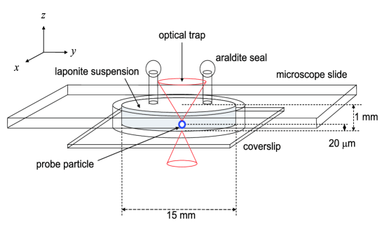
Figure 1: Diagram of the sample cell used during the experiment. The diagram is not in proper scale.

Physical properties of Laponite suspensions are very sensitive to the method used during their preparation [21]. Hence, an experimental protocol must be followed in order to perform reproducible measurements of their aging properties. Laponite RD, the most frequently studied grade and the one studied in this work, is a hygroscopic powder that must be handled in a controlled dry atmosphere. The powder is mixed with ultrapure water, at a weight concentration which has been varied from 1.2 to 3.0 %. The pH has been adjusted to 10 in order to assure chemical stability of the samples. At lower pH, the decomposition of clay particles occur. CO₂ absorption by water can modify the pH of the samples and then their aging properties. For these purposes, the preparation of the samples is done entirely within a glove box filled with circulating nitrogen. As we said the concentration is varied from 1.2 % to 3.0 % wt for different ionic strength. These conditions allow us to obtain either a gel or a glass according to the phase diagramm found in the literature [9]. At 2.8 % Laponite gelation takes place in few hours after the preparation. The suspension is vigorously stirred by a magnetic stirrer during 30 minutes. The resulting aqueous suspension is filtered through a 0.45 $\mu$m micropore filter in order to destroy large particle aggregates and obtain a reproducible initial state. The initial aging time ($t_{w}=0$) is taken at this step. Immediately after filtration, a small volume fraction (0.02 $\mu$l per 50 ml of sample) of silica microspheres (diameter = 2 $\mu$m) is injected into the suspensions. Microspheres play the role of probes to study the aging of the colloidal glass, as explained further. The sample is placed in a ultrasonic bath during 10 minutes to destroy small undesired bubbles that could be present during the optical tweezers manipulation. The suspension is introduced in a sample cell which is sealed in order to avoid evaporation and the use of vacuum grease, used in other experiments. Indeed this grease, whose pH is much smaller than 10, quickens the evolution of the suspension giving very strange and not reproducible results. Two kinds of completely sealed cells have been used. The first used one microscopic slide and a coverslip glued with Gene Frame adhesive spacers. This cell gives good results but the contact surface between the suspension and the adhesive is large. In order to decrease such contact surface we use more recently a sample cell consisting on a microscope slide and a coverslip separated by a cylindrical plastic spacer of inner diameter 15 mm, thickness 1 mm and glued together with photopolymer adhesive, as shown in Fig. 1. In this cell the inputs are sealed with araldite adhesive in order to avoid evaporation and direct contact with CO₂ from air.

2.2 Optical tweezers setup and data acquisition

We measure the fluctuations of the position of one or several silica beads trapped by an optical tweezers during the aging of the Laponite. The experiment is performed in a typical optical tweezers system at room temperature ($22\pm 1^{\circ}$ C).

2.2.1 Single Trap

The laser beam ($\lambda=$ 980 nm) is focused by a microscope objective ($\times$63) 20 $\mu$m above the coverslip surface to create a harmonic potential well where a bead of 1 or 2 $\mu$m in diameter ($2r$) is trapped. The power of the trapping beam is varied from 33 mW to 71 mW. With these laser intensities the surrounding liquid is heated of only a few degree. The position of the bead is detected by measuring with a 4 quadrant detector, the deflection of a He-Ne laser beam which is focused on the bead by the same microscope objective. The power of the measuring beam is only a few mW. The output signals of the 4 quadrant detector, which measures the positions $(x,y)$ of the bead, are acquired at a sampling frequency of 8196 Hz with 16-bit accuracy.

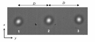
Figure 2: Configuration of three optical traps separated by a distance $D=9.3\times 10^{-6}$ m. The bright spots in the image correspond to three probe particles of 2 $\mu$m diameter trapped by them.

2.2.2 Multiple Trap

We use a Nd:YAG diode pumped solid state laser (Laser Quantum $\lambda=1064$ nm) whose beam is strongly focused by a microscope oil-immersion objective ($\times 63$, NA $=1.4$). The sample cell is placed on a piezoelectric stage (NanoMax-TS MAX313/M) in order to have mechanical control in three dimensions of nanometric accuracy during the trapping process. The sample cell is placed with the glass plate at the top and the coverslip at the bottom in such a way that the focus of the laser beam is located 20 $\mu$m above the coverslip inner surface (see Fig. 1). The whole system is mounted on an optical table in order to get rid of low frequency mechanical noise.

The light source used for detection is a halogen lamp whose beam is focused in the sample by a condenser lens. The halogen light passes through the sample and then the resulting interference contrast signal is detected by a high speed camera (Mikrotron MC1310) after emerging from the microscope objective. Once probe particles are trapped properly, images with a resolution of 240$\times$80 pixels are recorded at a sampling rate of 200 frames per second during 50 seconds and saved in AVI format every 97 seconds (i.e. 10000 images per AVI file) for further data processing. Hence, the aging time of the system $t_{w}$ is measured in multiples of 97 s while the smallest measurable time scale (the time elapsed between successive positions of the probe) corresponds to 5 ms and the highest accessible frequency is 100 Hz. We follow the trajectories of the trapped bead ($(x(t),y(t))$ on the focal plane by means of a MATLAB image processing program.

Multiple probe particles are needed to be trapped within the same sample in order to perform simultaneously passive and active microrheology measurements (see Sect. 3). Since two trapped particles are needed for each technique, at least three different optical traps must be created simultaneously, as shown in Fig. 2. For passive measurements, two traps of different stiffness and fixed positions are needed. We label the weakest trap as ’1’ while the strongest one as ’2’. For active measurements, one needs one trap in a fixed position in order to measure the power spectral density of displacement fluctuations. For convenience, we choose trap ’2’ for such purpose. In addition, one needs an oscillating trap in order to measure the response of the probe to an external forcing. This trap is labeled as ’3’. The separation distance between adjacent traps is $D=9.3\times 10^{-6}$ m, which is sufficiently large to avoid correlations between their motions. In the following, $x$ defines the direction along which the position of the optical trap is oscillated in time, while $y$ corresponds the orthogonal direction (see Fig. 2). For simplicity, all our calculations rely on $x$ coordinates only.

The creation of three optical traps on the $x-y$ plane is implemented by means of two coupled acousto-optic deflectors (AOD). In order to create three traps, the laser beam scans three different positions along the $y$ direction at a rate of 10 kHz. The scanning rate must be large enough in order to avoid the diffusive motion of the particle through the surrounding medium during the absence of the beam. The oscillation of the position of trap ’3’ is accomplished by deflecting the laser beam along $x$ with a given waveform $x_{0}(t)$ when it scans the position that it would visit in the absence of deflection along $x$. The stiffness of each trap is proportional to the time that the laser beam stays in the corresponding position. We check that by selecting a ratio of 20:40:40 for the visiting time of traps ’1’, ’2’ and ’3’, respectively we obtain a stiffness ratio of 20.7:39.7:39.6, respectively. Specifically the stiffness of the three traps are: $k_{1}=3.73\>\textnormal{pN}/\mu\textnormal{m}$, $k_{2}=7.15\>\textnormal{pN}/\mu\textnormal{m}$, $k_{3}=7.12\>\textnormal{pN}/\mu\textnormal{m}$. The stiffness has been measured using the power spectrum technique of Ref. [25].

3 Microrheology techniques

The determination of effective temperature, viscosity and elasticity of laponite samples during aging is done using microrheology. It consists on the measurement of the motion of probe particles embedded in the colloidal glass and manipulated by the optical tweezers system. This is the approach followed by [17, 18, 19] leading to conflicting results between passive and active measurements. There are two different kinds of microrheology techniques depending on the manipulation of the probes by the optical trap: passive and active.

In order to measure $T_{eff}$ for the particle motion several techniques have been used. The first one is based on the laser modulation technique as proposed in [18]. The second is based on the Kramers-Kronig relations with two laser intensities and it combines the advantages of two methods proposed in [22, 11] and in [18]. Finally the third method uses the advantages of several beads in a multi-traps tweezers and allows to apply the different techniques simultaneously.

3.1 Passive microrheology

In passive microrheology (PMR), an optical trap acts as a passive element keeping a bead in a fixed position while measuring the displacement fluctuations $x(t)$ to probe the properties of the medium.

In the present work, PMR measurements of effective temperature and elasticity of the colloidal glass are based on the method proposed by Greinert et al [18] This method is based on a generalization of the equipartition relation to glassy systems argued by Berthier and Barrat [23]. Since a Laponite suspension becomes viscoelastic as it ages, a probe particle immersed in it is subject to an additional force $F_{e}=-K_{Lap}x$ due to the elasticity of the colloidal glass, where $K_{Lap}$ denotes the effective elastic stiffness of the colloid. Then, by introducing an effective temperature $T_{eff}$ by means of the generalized equipartition relation

$${k_{B}\ T_{eff}\over(k+K_{Lap})}=\left<x^{2}-\left<x\right>^{2}\right>,$$ (3)

where brackets stand for average over the time (during a time window such that $K_{Lap}$ is almost constant). Note that this definition of effective temperature is global in frequency and then its measurement is strongly limited by the capability of detecting slow modes.

3.1.1 Laser intensity modulation technique

Following the method used in [18], the stiffness of the single optical trap is periodically switched between two different values ($k_{1}$ and $k_{2}$) every 61 seconds by changing the laser intensity. At a given $t_{w}$, on an interval of $60$ s we compute the variance of the position $\langle\delta x^{2}(t_{w})\rangle=\langle x^{2}-\left<x\right>^{2}\rangle$ on time windows of length 3 s $<\tau<$ 50 s. One must be aware that this time window is not sufficiently long to take into account the role of low frequency fluctuations at late stages during aging, and variances could be underestimated in this regime, as noted by [20] and in Sect. 4. The values of the variance computed in each window are then averaged over a 60 s interval, which is chosen sufficiently short to assure that the viscoelasticity of the colloidal glass remains almost constant, specifically :

$$\langle\delta x^{2}(t_{w})\rangle_{j}={1\over\tau t_{max}}\int_{t_{w}}^{t_{w}+t_{max}}dt\int_{t}^{t+\tau}(x_{j}^{2}(t^{\prime})-\langle x_{j}(t^{\prime})\rangle^{2})dt^{\prime},$$ (4)

where $t_{max}=60$ s and $\langle\delta x_{j}^{2}(t_{w})\rangle$ with $j=1,2$ correspond to the variance measured with $k_{1}$ and $k_{2}$ respectively. To avoid transient each record is started 20 s after the laser switch to be sure that the system has relaxed toward a quasi stationary state. Assuming the equipartition principle Eq. (3) still holds in this out-of-equilibrium system, $T_{eff}$ is computed as in [18]. The expressions of the effective temperature and of the Laponite elastic stiffness $K_{Lap}$ are the following

$$k_{B}T_{eff}={(k_{2}-k_{1})\langle\delta x^{2}(t_{w})\rangle_{1}\langle\delta x^{2}(t_{w})\rangle_{2}\over\langle\delta x^{2}(t_{w})\rangle_{1}-\langle\delta x^{2}(t_{w})\rangle_{2}},$$ (5)

$$K_{Lap}={k_{1}\ \langle\delta x^{2}(t_{w})\rangle_{1}-k_{2}\langle\delta x^{2}(t_{w})\rangle_{2}\over\langle\delta x^{2}(t_{w})\rangle_{1}-\langle\delta x^{2}(t_{w})\rangle_{2}}.$$ (6)

We notice that when multiple traps are used there is no need to modulate the laser as the stiffness of the trap ’1’ and ’2’ in Fig. 2 are respectively $k_{1}$ and $k_{2}$. Thus the method is immediately implemented using these two beads. The only difference is that now the acquisition frequency is 200 Hz. But there are several advantages here. The two variances at $k_{1}$ and $k_{2}$ are computed simultaneously and since the power of the laser is not commuted there are neither temperature variation inside the sample nor dead time of 20 s. Thus the measurement of the variance can be done each 60 s. In this way the results are cleaner than with a single bead.

This technique, although quite interesting and simple, has several drawbacks that we will discuss in the next sections. Furthermore, being a global measurement, it has no control of what is going on on the different frequencies. To overcome this problem we have implemented the following method, which can be used only with a single bead due to the need of a large sampling frequency.

3.1.2 Kramers-Kronig and modulation technique

This combines the laser modulation technique described in the previous section and the passive rheology technique based on Kramers-Kronig relations. The fluctuation dissipation relations relate the spectrum $S_{j}(\omega)$ of the fluctuation of the particle position to the imaginary part $\chi_{j}^{\prime\prime}$ of the response of the particle to an external force, specifically :

$$S_{j}(\omega,t_{w})={4\ k_{B}T_{eff}\over\omega}\chi_{j}^{\prime\prime}(\omega,t_{w}),$$ (7)

with $j=1$ and $j=2$ for the spectra measured with the trap stiffness $k_{1}$ and $k_{2}$ respectively. We recall that for a particle inside a newtonian fluid $G=1/\chi_{j}=k_{j}+i\gamma\omega$ with $\gamma=6\pi\eta r$ the drag coefficient and $\eta$ the fluid viscosity. In Eq. (7) the dependence in $t_{w}$ takes into account the fact that the properties of the fluid changes after the preparation of the Laponite suspension. If one assumes that $T_{eff}$ is constant as a function of frequency (hypothesis that can be easily checked a posteriori) then the real part $\chi_{j}^{\prime}$ of the response is related to $\chi_{j}^{\prime\prime}$ by the Kramers-Kronig relations [22] that is:

$$\hat{\chi}_{j}^{\prime}(\omega,t_{w})={2\over\pi}P\int_{0}^{\infty}{\xi\hat{\chi}^{\prime\prime}(\xi,t_{w})\over\xi^{2}-\omega^{2}}d\xi={1\over 2\pi k_{B}T}P\int_{0}^{\infty}{\xi^{2}S_{j}(\xi,t_{w})\over\xi^{2}-\omega^{2}}d\xi,$$ (8)

where $P$ stands for principal part of the integral and $\hat{\chi}_{j}^{\prime}$ is computed assuming that $T_{eff}$ does not depend on the frequency in the second equality where we have used Eq. (7), i.e. $\hat{\chi}^{\prime\prime}(\xi,t_{w})=\omega S_{j}(\omega,tw)/(4k_{B}T)$. To compute $\hat{\chi}_{j}^{\prime}$ from Eq. (8) we use a Fourier transform algorithm that is:

$$\hat{\chi}_{j}^{\prime}(\omega,t_{w})={1\over 2\pi k_{B}T}\int_{0}^{1/\omega_{min}}\cos(\omega\ t)\ dt\ \int_{0}^{\omega_{max}}\xi^{2}S_{j}(\xi,t_{w})\ \sin(\xi\ t)d\xi,$$ (9)

where $\omega_{min}$, $\omega_{max}$ are the minimum and maximum frequencies resolved in $S_{j}(\omega)$. Mathematically one should have $\omega_{min}=0,\omega_{max}=\infty$. However this is not possible experimentally and the limited interval $[\omega_{min},\omega_{max}]$ induced an error in the high frequency estimation of $\hat{\chi}_{j}^{\prime}$. This error can be easily estimated and one evaluates that the values of $\chi^{\prime}$ are correct within a few percent for $\omega\leq\omega_{max}/10$. Once $\hat{\chi}_{j}^{\prime}$ has been computed from Eq. (9) then one can compute $\hat{G}_{j}=1/(\hat{\chi}_{j}^{\prime}+i\hat{\chi}_{j}^{\prime\prime})$, where $\hat{\chi}^{\prime\prime}$ is computed from Eq. (7) with $T_{eff}=T$. Obviously the real part of $G$ is given by:

$$G_{j}^{\prime}(\omega,t_{w})=k_{j}+K_{Lap}(\omega,t_{w})={T_{eff}(\omega,t_{w})\over T}\hat{G}_{j}^{\prime}(\omega,t_{w}).$$ (10)

Using the two measurements at $k_{1}$ and $k_{2}$ one can solve for $K_{Lap}$ and $T_{eff}$ getting:

$$K_{Lap} = {k_{1}\ \hat{G}^{\prime}_{2}(\omega,t_{w})-k_{2}\ \hat{G}^{\prime}_{1}(\omega,t_{w})\over\hat{G}^{\prime}_{1}(\omega,t_{w})-\hat{G}^{\prime}_{2}(\omega,t_{w})},$$ (11)

$$T_{eff}(\omega,t_{w}) = T\left({k_{1}-k_{2}\over\hat{G}^{\prime}_{1}(\omega,t_{w})-\hat{G}^{\prime}_{2}(\omega,t_{w})}\right).$$ (12)

It is clear that if one finds a dependence of $T_{eff}$ on $\omega$ this method cannot be used because $\chi^{\prime\prime}(\omega,t_{w})$ is not simply proportional to $S_{j}(\omega,t_{w})\omega$ as assumed in Eq. (8). This method is very sensitive to the shape of the spectrum and to its statistical noise. Thus, before computing the elastic modulus, we smooth the spectra to reduce the statistical uncertainty.

3.2 Active microrheology

Active microrheology (AMR) involves the active manipulation of probe particles by an external force exerted by optical tweezers. In our case, we apply an oscillatory force $f_{0}(t,\omega)$ at certain frequencies $\omega$ by means of the spatial modulation $x_{0}(t,\omega)$ of trap ’3’. One determines the Fourier transform of the linear response function:

$$\hat{\chi}(\omega,t_{w})=\frac{\hat{x}(\omega,t_{w})}{\hat{f}_{0}(\omega)},$$ (13)

in order to resolve the viscoelastic properties of the colloidal suspension.

As mentioned before, there are a priori two times scales in the glassy system. The viscoelastic properties evolve in a slow aging time $t_{w}$ ($\gamma=6\pi r\eta=\gamma(\omega,t_{w})$, $K_{Lap}=K_{Lap}(\omega,t_{w})$) while displacements fluctuations evolve in the fast time scale $t\ll t_{w}$. The effective hookean force on the particle due the relative displacement $x(t)-x_{0}(t,\omega)$ with respect to the laser beam focus is $-k_{3}(x(t)-x_{0}(t,\omega))$ while the force due the evolving elasticity of the medium is $-K_{Lap}(\omega,t_{w})x(t)$. Hence, the motion of the probe particle is described by the following Langevin equation

$$\gamma(\omega,t_{w})\dot{x}+k_{3}(x-x_{0}(t,\omega))+K_{Lap}(\omega,t_{w})x=\sqrt{2k_{B}T_{eff}(\omega,t_{w})\gamma(\omega,t_{w})}\xi(t).$$ (14)

In order to derive a relation between the linear response function and the frequency-dependent viscoelastic properties of the colloidal glass, Eq. (14) must be recasted with no stochastic term, as

$$\gamma(\omega,t_{w})\dot{x}+(k_{3}+K_{Lap}(\omega,t_{w}))x=f_{0}(t,\omega),$$ (15)

where $f_{0}(t,\omega)=k_{3}x_{0}(t,\omega)$ is the active force term. The Fourier transform of Eq. (15) is computed over a time window of 10 s (such that $\gamma$ and $K_{Lap}$ are constant) and moving-averaged over 50 seconds. It leads to the following expression for the inverse of the response function at given frequency and aging time

$$\frac{1}{\hat{\chi}(\omega,t_{w})}=i\omega\gamma(\omega,t_{w})+(k_{3}+K_{Lap}(\omega,t_{w})),$$ (16)

Therefore, by measuring directly the mechanical response at a given frequency of the particle motion to the applied external force, it is possible to resolve either the relative viscosity and the elasticity of the colloidal glass during aging by means of the expressions

$$\frac{\omega\gamma(\omega,t_{w})}{k_{3}}=Im\{\frac{1}{k_{3}\hat{\chi}(\omega,t_{w})}\},$$ (17)

$$\frac{K_{Lap}(\omega,t_{w})}{k_{3}}=Re\{\frac{1}{k_{3}\hat{\chi}(\omega,t_{w})}\}-1.$$ (18)

In our case, the position of trap ’3’ is oscillated in time along the $x$ direction at three different frequencies $\omega=\omega_{j},j=1,2,3$ simultaneously according to

$$x_{0}(t,\omega)=A(\sin(\omega_{1}t)+\sin(\omega_{2}t)+\sin(\omega_{3}t)),$$ (19)

where $f_{1}=\omega_{1}/2\pi=0.3$ Hz, $f_{2}=\omega_{2}/2\pi=0.5$ Hz, $f_{3}=\omega_{3}/2\pi=1.0$ Hz, and $A=9.2\times 10^{-7}$ m. Higher frequency sinusoidal oscillations ($\omega/2\pi=$ 2.0, 4.0, 8.0 Hz) were also checked in order to compare our results at low frequencies to higher ones.

AMR allows to determine directly the effective temperature of the colloidal glass at given frequency $\omega$ and aging time $t_{w}$ by means of Eq. (2), as suggested by [17]. First of all, one needs to synchronize the input forcing signal $x_{0}(t,\omega)$ with the response of the trapped bead $x(t)$. The Fourier transform of the response function is determined by using Eq. (13) for a probe particle driven by trap ’3’: in practice we divide the power spectral density of the output signal $|\hat{x}(\omega,t_{w})|^{2}$ by the corresponding transfer function $\hat{x}^{*}(\omega,t_{w})\hat{f}_{0}(\omega)$. On the other hand, one needs to determine the power spectral density of the displacement fluctuations in the absence of external forcing but for the same value of the trapping stiffness. For this reason, traps ’2’ and ’3’ are created with the same stiffness. We measure the power spectral density of fluctuations of a particle kept by trap ’2’.

4 Experimental results of the single bead experiment

4.1 Laser modulation method

Fig. 3(a) shows the power spectra of the particle fluctuations inside Laponite at concentration measured at four different $t_{w}$ with the trap stiffness $k_{1}=6.34$ pN/$\mu$m. We see that as time goes on the low frequency component of the spectrum increases. That is the cut-off frequency $(k_{j}+K_{Lap})/\gamma$ decreases mainly because of the increasing of the viscosity. At very long time this cut-off is well below 0.1 Hz. In Fig. 3(b) we plot the variance of the particle measured for the same data of Fig. 3(a) on time windows of length $\tau=61$ s. The variances remain constant for a very long time and they begin to decrease because of the increase of the gel stiffness. Using these data and Eq. (5) and Eq. (6) one can compute $T_{eff}$ and $K_{Lap}$. The results for $T_{eff}$ and $K_{Lap}$ are shown in Fig. 4(a) and 4(b) respectively.

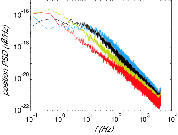
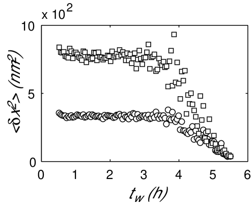
Figure 3: (a) Spectra of the particle position fluctuations inside a Laponite solution at $2.3\%$ wt. The spectra has been measured for the trap stiffness $k_{1}=6.34$ pN/$\mu$m at various ageing times: from right to left $t_{w}=30$, $110$, $190$ and $270$ minutes. (b) Evolution of $\left<\delta x^{2}\right>$ with $t_{w}$ for both stiffness, $k_{1}=6.34$ pN/$\mu$m ($\square$) and $k_{2}=14.4$ pN/$\mu$m, ($\circ$). The variances have been measured on a time window of $\tau=61$ s.

We find that $T_{eff}$ is constant at the beginning and is very close to $T_{bath}=294$ K, then when the jamming occurs, that is when $K_{Lap}$ increases, it becomes more scattered without any clear increase with $t_{w}$, contrary to Ref. [18]. We now make several remarks. First, we point out that the uncertainty of their results are underestimated. The error bars in Fig. 4(a) are here evaluated from the standard deviation of the variance using Eq. (2) in Ref [18] at the time $t_{w}$. Although they are small for short time $t_{w}$, ($\Delta T_{eff}/T_{eff}\leq 10\%$), they increase for large $t_{w}$. This is a consequence of the increase of variabilities of $\left<\delta x_{j}^{2}\right>$ as the colloidal glass forms. This point is not discussed in in Ref. [18] and we think that the measurement errors are of the same order or larger than the observed effect. The results depend on the length of the analyzing time window and the use of the principle of energy equipartition becomes questionable for the following reasons.

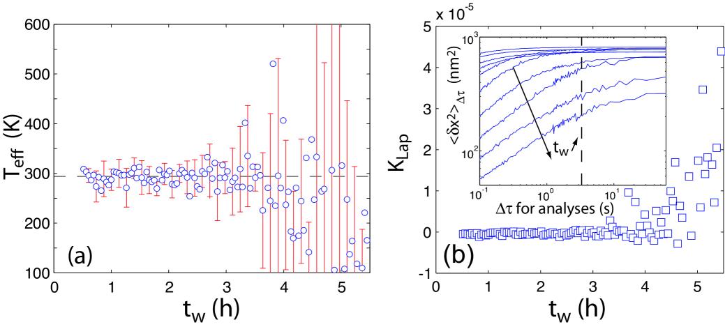
Figure 4: (a) Evolution of the effective temperature with aging time for the data of Fig. 3 $k_{1}=6.34$ pN/$\mu$m, $k_{2}=14.4$ pN/$\mu$m, 2.3% wt of Laponite and $r=$ 1 $\mu$m glass bead. The error bars are computed from the statistical error of $\left<\delta x_{j}^{2}\right>$ at the time $t_{w}$. (b) Evolution of the stiffness of the Laponite with ageing time. Inset: Evolution of $\left<\delta x^{2}\right>_{\Delta\tau}$ for $k_{1}=6.34$ pN$/\mu$m as a function of the duration $\Delta\tau$ of the samples for different aging times : $t_{w}=30$, $57$, $83$, $110$, $137$, $163$, $190$, $217$, $243$ and $270$ minutes.

First, these analyzing windows cannot be made too large because the viscoelastic properties of Laponite evolve as a function of time. Second, the corner frequency of the global trap (optical trap and gel), the ratio of the trap stiffness to viscosity, decreases continuously mainly because of the increase of viscosity. At the end of the experiment, the power spectrum density of the displacement of the bead shows that the corner frequency is lower than 0.1 Hz. We thus observe long lived fluctuations, which could not be taken into account with short measuring times. This problem is shown on Fig. 4(b). We split our data into equal time duration $\Delta\tau$, compute the variance and average the results of all samples. The dotted line represents the duration 3.3 s chosen in [18]. At the beginning of the experiment, the variance of the displacement is constant for any reasonable durations of measurement. However, we clearly see that this method produces an underestimate of $\left<\delta x^{2}\right>$ for long aging times, specially when the viscoelasticity of the gel becomes important. Long lived fluctuations are then ignored.

Moreover, in some experiments, we observe a small drift of the probe position at the end of the measurements, when the gel stiffness becomes very large compared to the optical trap stiffness. Figure 5(a) shows an example of the time evolution of the mean position of a single trapped bead. The first drift is associated to the evolution of the temperature inside the sample due to the laser. After 3.5 hours, the mean position of the bead is less accurate, which is the consequence of the increase of the viscosity of the Laponite as mentioned above, but we can observe a drift toward larger values of $x$. This phenomenon can be enhanced, using smaller beads in a Laponite sample at higher concentration and higher ionic strength. We simultaneously measure the positions of three beads of 1 $\mu$m in diameter in three fixed traps. The beads start escaping their trap after 90 min. In Figure 5(b), we compare the trajectory of the first particle with the third one. Even if the trajectories are not correlated over short times (1 s for a pincushion), at longer time, the drift is identical for both beads. This global drift is in this case obviously an artifact that could be due to a small leak or a small bubble. We point out here that data needs careful analysis to get rid of strange behavior.

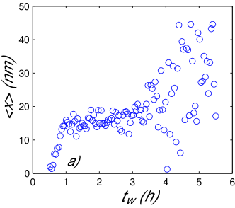
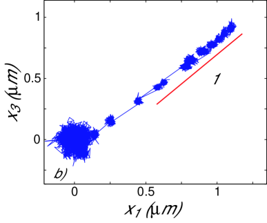
Figure 5: (a) Evolution of the mean position along the $x$-direction with aging time, same data as in Fig. 3. (b) Comparison of the trajectories for two $1\mu$m in diameter glass beads of whose fixed traps are separated by 6.5 $\mu$m during the evolution of the suspension of Laponite ($I=5\times 10^{-3}$ mol l^-1, 1.2% wt of Laponite). Each pincushion represents 1 second of measurement at 288 Hz, repeated every 5 min during 150 min.

4.2 Kramers-Kroening and modulation technique

This new method, using Kramers-Kronig relation, allows us to test the dependence of the effective temperature on the frequency. As we already mentioned, before applying Eq. (9) to the spectral data we proceed to a smoothing of the spectra $S_{j}(\omega)$. This operation is shown in Fig. 6. Then, instead of directly computing $\hat{\chi}_{j}^{\prime}(\omega,t_{w})$ using Eq. (9), we use the derivative of the inverse Fourier transform of the smoothed spectra. The artificial undulations of the smoothed spectra produce fluctuations on the final curves. To decrease this effect, we additionally fit the inverse Fourier transform by a stretched exponential function. These methods give finally results that are less sensitive to the noise of the spectra. We also check that this method produces spectra in agreement with the first ones (inset of Fig. 6) up to the limit of 100 Hz.

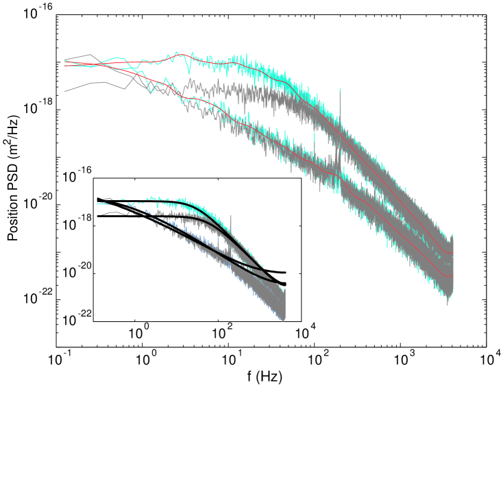
Figure 6: Example of spectral data and smooth spectra used with the Kramers-Kroenig relation ($k_{1}$ = 7.47 pN/$\mu$m, ${k_{2}}$ = 16.7 pN/$\mu$m and for two ageing times: ${t_{w}=}$ 30 min and 240 min) The red smooth lines of the main plot are obtained by averaging the spectra over fixed windows. Inset: We check that the position PSD deduced after data treatment (black thick lines) agree with the noisy spectra up to $10^{2}$ Hz (see text).

Figure 7(a) shows the real part of $G$, which corresponds to the global elastic modulus of the gel and of the laser, for both trap stiffness. The increase with time of $G^{\prime}$ is consistent with the increase of the strength of the gel. The elastic behavior of Laponite is also more pronounced at high frequency. The last decrease of the curves at very high frequencies is due to the numerical method. Indeed, the frequency cutoff should be set at least a decade below the frequency of the data acquisition: data above 200 Hz is not reliable. We see that the curves of each stiffness are well separated except at the end of the measurement, where the results are not accurate due to the large difference between the optical stiffness and Laponite stiffness.

From these data, we compute the ratio of the effective temperature to the bath temperature along the ageing process. These results are shown on Fig. 7(b) for three different frequencies ($f=1$ Hz, 10 Hz and 100 Hz). We first note that the three curves are almost identical. This means that the effective temperature does not depend on frequency. Second, the temperature ratio is close to 1. The dispersion of the data is rather small at early times and again increases when the stiffness of the gel overcomes those of the optical traps. This comes from the uncertainties of the elastic modulus which become larger than the difference between the two curves. This dispersion may also give negative temperatures for very long aging time, not shown in Fig. 7(b) which is an expanded view. Even if this method is less accurate than the previous one, it allows us to verify that the effective temperature is the same for all frequencies.

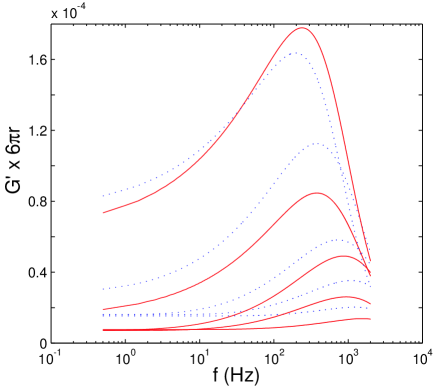
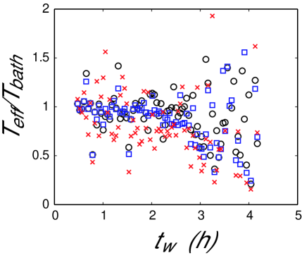
Figure 7: (a) Evolution of $6\pi rG^{\prime}$ (the global elastic modulus) as a function of frequency for both trap stiffnesses, $k_{1}=7.47$ pN/$\mu$m (solid lines), $k_{2}=16.7$ pN/$\mu$m (dashed lines) and for increasing aging time: $t_{w}=30$ min, $90$ min, $140$min, $190$ min and $240$ min (1.2% wt of Laponite, 2 $\mu$m glass bead and ionic strength $I=5\times 10^{-3}$ mol l^-1). (b) Evolution of the ration $T_{eff}/T_{bath}$ with aging time ($t_{w}$) for different frequencies ($f=1$ Hz $\square$, 10 Hz $\circ$ and 100 Hz $\times$)).

5 Results of the multiple trap experiment

In this section, unless otherwise stated, we will describe only the results obtained at 2.8 % wt concentration of Laponite. Indeed at this concentration the Laponite gelation occurs in a few hours.

5.1 Viscoelastic properties of the aging colloidal glass

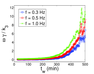
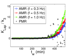
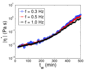
Figure 8: (a) Time evolution of viscosity of the colloidal glass obtained by means of AMR. (b) Time evolution of elasticity of the colloidal glass obtained either by PMR and AMR. (c) Time evolution of the modulus of the complex viscosity

We first present separately the results of the time evolution of viscosity and elasticity of the colloidal glass during aging. The time evolution of the dimensionless quantity $\omega\gamma/k_{3}$, linearly proportional to the dynamic viscosity $\eta$ of the colloidal glass, is shown in Fig. 8(a). As expected, it increases continuously as the system ages. On the other hand, the evolution of the stiffness $K_{Lap}$ is qualitatively different, as shown in Fig. 8(b). For $t_{w}<300$ min, $K_{Lap}\approx 0$, revealing an entirely viscous nature of the laponite suspension, while for $t_{w}>300$ min it becomes viscoelastic, with $K_{Lap}$ increasing dramatically in aging time from 0 to 10 times the stiffness of the second trap $k_{2}=7.15$ pN/$\mu$m. Both PMR and AMR lead to consistent and complementary results and we notice that AMR measurements are more accurate, leading to a very small dispersion of data around the mean trend. Instead, PMR measurements become very sensitive to the inverse of the difference $\langle\delta x^{2}\rangle_{1}-\langle\delta x^{2}\rangle_{2}$ as $t_{w}$ increases, leading to increasingly large data dispersion for $t_{w}>350$ min. In order to compare our AMR results with previous rheological measurements, in Fig. 8(c) we plot the time evolution of the modulus of the complex viscosity, given by $|\eta^{*}|=(\gamma^{2}+K_{Lap}^{2}/\omega^{2})^{1/2}/6\pi R$. We observe that $|\eta^{*}|$ increases, almost exponentially, of two orders of magnitude during the first 500 minutes of aging. The behavior of $|\eta^{*}|$ is in good agreement with previous rheological measurements [24].

5.2 Properties of non-equilibrium fluctuations during aging

The probability density functions of displacement fluctuations around their mean positions $\delta x=x-\langle x\rangle$, computed for particles ’1’ and ’2’ over an analyzing time window $\Delta\tau=$ 25 s, are Gaussian, as shown in Fig. 9(a) for particle ’2’. The corresponding variances $\langle\delta x^{2}\rangle_{1}$ and $\langle\delta x^{2}\rangle_{2}$ decrease during aging due to the combined effects of the increasing viscosity and elasticity of the colloid constraining the motion of the probe particles. The values of variances depend on the length of the analyzing time window $\Delta\tau$ and for very short windows, they become largely underestimated as the system evolves, as discussed in Subsection 4.1.

In order to go deeper into the artifacts that can arise for PMR from the use of very short windows, we analyzed the experimental data using for two different values $\Delta\tau=$ 3 s and 25 s. Fig. 9(b) shows the results for $\Delta\tau=$ 3 s. Two regimes can be identified like in previous PMR experiments [18], [20]: for $t_{w}\lesssim 300$ min, both variances are quite constant, while for $t_{w}\gtrsim 300$ min they decrease up to one order of magnitude at $t_{w}=500$ min. The transition between one regime to the other is kind of abrupt and occurs at $t_{w}\approx 300$ min $\equiv t_{g}$. This time corresponds to the transition from a purely viscous liquid-like phase to the formation of a viscoelastic glassy phase associated to the house of cards structure, as shown previously. It is noticeable that the transition point from the plateau to the decaying curve depends slightly on the value of the stiffness of the optical trap. We observe that the transition occurs first (around $t_{w}=250$ min) for the weakest trap (’1’) than for the strongest one (’2’) (around $t_{w}=300$ min), indicating that the motion of a probe particle could be sensitive to the relative strength of the optical trap with respect to the elasticity of the colloidal glass close to the gelation point. However, this is nothing but an artifact due to the use of a very short analyzing time window. Since the corner frequency of the power spectral density of displacement fluctuations depends linearly on the stiffness of the optical trap $k$, large underestimates of the corresponding variance occur first for the weakest trap when using $\Delta\tau=$ 3 s, leading to an apparent dependence of the onset of gelation on $k$. In fact, when using $\Delta\tau=$ 25 s, there is no such dependence as shown in Fig. 9(c). Even when smaller data variability is observed for $\Delta\tau=$ 3 s than for 25 s, one must be aware that the latter case is more reliable than the former since longer lived modes are taken into account in a method which must integrate the contributions of as many frequencies as possible.

Another artifact can arise easily due to wrong data smoothing. Figs. 9(b) and 9(c) also show the smooth curves resulting from the convolution of the data points of the variances with rectangular time windows of different lengths: 16 min in Fig. 9(b) and 5 min in Fig. 9(c). Wrong estimates become important at late aging times because of the use of an inappropriate moving window, like in the case of the window of 16 min.

Both artifacts can lead to an apparent systematic increase of the effective temperature of the colloid, as shown in Subsection 5.3. Hence, one must be very careful when analyzing experimental data using PMR for a non-ergodic system such as the colloidal glass studied here.

Frequencies as low as 0.1 Hz could be resolved properly using the multitrap method, as shown in the spectral curves of displacement fluctuations of particles ’2’ and ’3’ (Fig. 9(d)). The application of the oscillating force $f_{0}(t,\omega)$ on particle ’3’ leads to an increase of two orders of magnitude of its spectrum at the corresponding frequency $\omega$. Hence, both the power spectral density and the response function could be measured with good frequency resolution in the case of AMR. Fig. 9(e) shows the time evolution of the power spectral density for each frequency studied $\omega=\omega_{j},j=1,2,3$. The time behavior of $|\hat{x}(\omega,t_{w})|^{2}$ is completely different from that of ergodic liquids at equilibrium, whose value is constant in time. We observe that the nontrivial shape of the power spectral density has a maximum which depends on the value of the corresponding frequency. Fig. 9(f) shows the time evolution of the imaginary part of the Fourier transform of the response function at each frequency $\omega=\omega_{j},j=1,2,3$, calculated by means of Eq. (13). We observe the same behavior in time for each frequency, indicating that $|\hat{x}(\omega,t_{w})|^{2}$ and $Im\{\hat{\chi}(\omega,t_{w})\}$ are related by a proportionality constant during aging, satisfying a generalized FDT relation (Eq. (2) with no dependence on $t_{w}$), as explained in in the next section. It has to be noted that the position of these maxima depend on the strength of the optical traps used to measure the response and fluctuations. These strengths are the same in our case whereas they are different in the experiment of Ref. [16] where the fluctuations have been measured on free particles. This difference in the strength induces a shift on the time position of these maxima which must be corrected in the data analysis. Small errors in this correction may of course induce an anomalous maximum of $T_{eff}$ as it has been reported in [16].

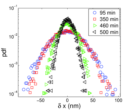
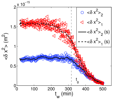
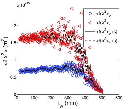
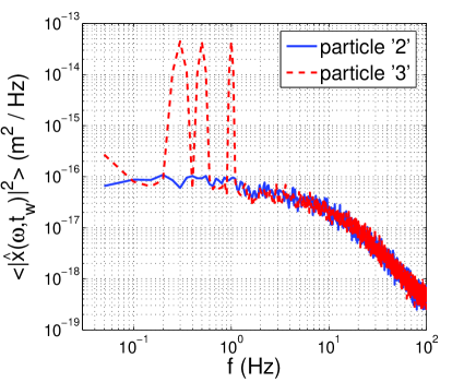
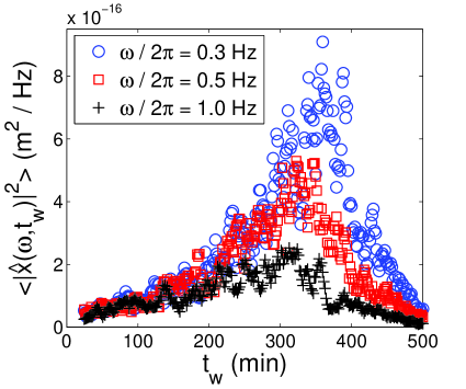
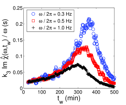
Figure 9: (a) PDFs of $\delta x$ at different $t_{w}$ for particle ’2’. (b) Time evolution of variances for particles ’1’ and ’2’ computed for $\Delta\tau=3$ s. The thin dashed line indicates the approximate aging time when gelation begins to take place. Labels (s) correspond to smooth curves (see text). (c) Time evolution of variances computed for $\Delta\tau=25$ s. (d) Spectra of displacement fluctuations of particles ’2’ and ’3’ at $t_{w}=$ 95 min. (e) Time evolution of the power spectral densities of displacement fluctuations of particle ’2’ for the three frequencies studied. (f) Time evolution of the imaginary part of the Fourier transform of the response functions of particle ’3’.

5.3 Effective temperatures

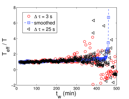
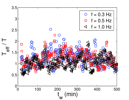
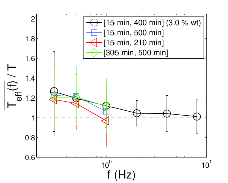
Figure 10: (a) Time evolution of effective temperatures of the colloid during aging obtained by means of PMR (see text for symbols). (b) Time evolution of effective temperatures for different frequencies obtained by means of AMR. (c) Aging time average of the effective temperatures obtained by AMR for different frequencies. Error bars represent the standard deviation of data shown in Fig. 10(b).

Effective temperatures obtained by means of both PMR and AMR are shown in Figs. 10(a) and 10(b), respectively. In the case of PMR, for $t_{w}<250$ min the effective temperature is very close to the bath temperature $T=295$ K with very few data dispersion around it. This is due to the fact that at this aging stage the aqueous laponite suspension behaves as a viscous liquid leading to small and constant data dispersion of $\langle\delta x^{2}\rangle$. However, for 250 min $<t_{w}$ the behavior of $T_{eff}$ depends on the lengths of the moving time windows used to compute the displacement variances and to smooth data. As discussed previously, the most reliable results are obtained by using a sufficiently long analyzing window ($\Delta\tau=$ 25 s) and a sufficiently short smoothing window (5 min). In this case no systematic increase of the effective temperature around the bath temperature is observed even when the suspension has already gelified (300 min $<t_{w}<$ 350 min), but data dispersion becomes very large as $t_{w}$ increases (triangles in Fig. 10(a)). On the other hand, for $\Delta\tau=$ 3 s and a smoothing window of 5 min, we observe an apparent increase of the effective temperature for 200 min $<t_{w}<$ 350 min (circles), corresponding to the stage when underestimates of the variance occur first for the weakest trap. Once again, we observe an increasing variability of the effective temperature leading even to negative values of $T_{eff}$ due to the fact that the dispersions of $\langle\delta x^{2}\rangle_{1}$ and $\langle\delta x^{2}\rangle_{2}$ are comparable to $\langle\delta x^{2}\rangle_{1}-\langle\delta x^{2}\rangle_{2}$. Finally, for $\Delta\tau=$ 3 s and a smoothing window of 16 min, a dramatic increase of the effective temperature is observed for $t_{w}>$ 400 min (squares). This is very similar to the behavior of $T_{eff}$ reported by [18] and we assert that such increase is not an actual violation of FDT but the result of both the underestimates of the variances and inappropriate data smoothing.

The AMR results for the effective temperature at different frequencies are shown in Fig. 10(b). We verify that there is no actual systematic increase of $T_{eff}$ as the colloidal glass ages. The effective temperatures recorded by the probe particles subject to the non-equilibrium fluctuations in the colloidal glass at a given time scale $1/\omega$ are equal to the bath temperature during aging even for the slowest modes studied ($\sim 1/f_{1}\approx 3$ s). Unlike PMR measurements, we find that the variability of the data is constant in aging time, which implies that AMR is a more reliable method even during gelation. In order to check if $T_{eff}(\omega,t_{w})=T$ within experimental accuracy, by taking into account the constant behavior of $T_{eff}$ and of the dispersion around its mean value we can compute the aging time average of $T_{eff}(\omega,t_{w})$ over different aging time intervals $t_{w}\in[t_{w}^{i},t_{w}^{f}]$

$$\overline{T_{eff}(\omega)}=\frac{1}{t_{w}^{f}-t_{w}^{i}}\int_{t_{w}^{i}}^{t_{w}^{f}}T_{eff}(\omega,t_{w}^{\prime})dt_{w}^{\prime},$$ (20)

for every frequency $\omega$. Fig. 10(c) shows the results of $\overline{T_{eff}(\omega)}$ with their respective error bars corresponding to the standard deviations of the data sets. For comparision, we also determined the effective temperature of the colloidal glass at 3.0% wt of Laponite at higher frequencies ($f=$ 2.0, 4.0 and 8.0 Hz) without observing any deviation of the effective temperatures from the bath temperature within experimental accuracy (Fig. 10(c)). We conclude that there is no violation of FDT for this aging non-equilibrium system with its effective temperatures equal to the bath temperature, regardless of the measured time scale.

5.4 Probability density functions of heat fluctuations

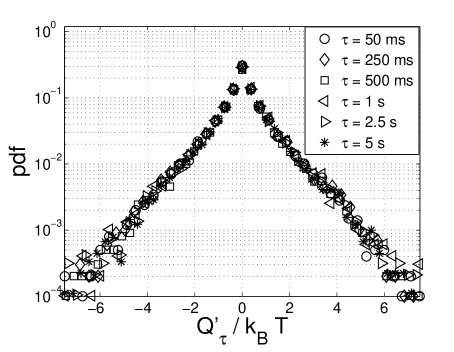
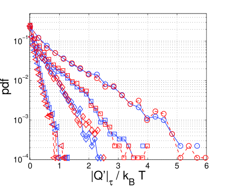
Figure 11: (a) PDFs of $Q^{\prime}_{\tau}$ at $t_{w}=95$ min for different values of $\tau$. (b) PDFs of $|Q^{\prime}_{\tau}|$ for $\tau=5$ s at different aging times $t_{w}$ after the onset of gelation (from top to bottom: $t_{w}=340$, $435$, $470$ and $500$ min). Blue points correspond to $Q^{\prime}_{\tau}>0$ while red ones to $Q^{\prime}_{\tau}<0$.

Finally, we present the results for the probability density functions (PDF) of heat transfers between the colloidal glass and the surroundings. This kind of analysis has been motivated by the recent experimental works on fluctuations of injected and dissipated power in systems with harmonic [26, 27] and non harmonic potential [28, 29] within the context of fluctuations theorem (FT) (see [30] for a review on FT). The idea of using FT for theoretically studying the heat flux in aging systems has been first proposed in [31, 32]. Let us summarize the main physical concepts that are behind this idea. Since non-equilibrium fluctuating forces due to the collisions of the colloidal glass particles with a micron-sized probe particle do work $W_{\tau}$ (of ensemble average $\langle W_{\tau}\rangle=0$) on it in a given time interval $\tau$, a fraction of $W_{\tau}$ must be dissipated in the form of heat $Q_{\tau}$. $Q_{\tau}$ is a stochastic variable which may be either positive (heat received by the probe) or negative (heat transferred to the colloid). In an ergodic system acting as an equilibrium thermal bath at temperature $T$, the mean heat transfer must vanish $\langle Q_{\tau}\rangle=0$ in the absence of any external forcing on the probe in order to satisfy the first law of thermodynamics. However, in a system out of equilibrium this situation is not necessarily fulfilled due to non-ergodicity. A mean heat transfer $\langle Q_{\tau}\rangle>0$ would be a signature of an effective temperature of the colloidal glass $T_{eff}(\omega,t_{w})>T$ during a time lag $\tau\approx 2\pi/\omega$. Hence, by investigating possible asymmetries in the PDF of $Q_{\tau}$ for different time lags and at different aging times, one could find possible violations of FT in the aging colloidal glass.

In order to calculate the heat transfer during a time lag $\tau$, Eq. (14) (with $x_{0}(t,\omega)=0$ since we are interested in the situation without any external forcing) is multiplied by $\dot{x}$ and integrated from $t_{w}$ to $t_{w}+\tau$ (with $\tau\ll t_{w}$), leading to an extension of the first law of thermodynamics for a probe particle subject to non-equilibrium thermal fluctuations of the colloidal glass

$$\Delta U_{\tau}(t_{w})=Q_{\tau}(t_{w}),$$ (21)

where

$$\Delta U_{\tau}(t_{w})=\frac{1}{2}(k+K_{Lap}(t_{w},\frac{2\pi}{\tau}))(x(t_{w}+\tau)^{2}-x(t_{w})^{2}),$$ (22)

and

$$Q_{\tau}(t_{w})=-\gamma(t_{w},\frac{2\pi}{\tau})\int_{t_{w}}^{t_{w}+\tau}\dot{x}(t^{\prime})^{2}dt^{\prime}+\sqrt{2k_{B}T_{eff}(t_{w},\frac{2\pi}{\tau})\gamma(t_{w},\frac{2\pi}{\tau})}\int_{t_{w}}^{t_{w}+\tau}\xi(t^{\prime})\dot{x}(t^{\prime})dt^{\prime}.$$ (23)

In practice we determine the PDF of the stochastic variable $Q^{\prime}_{\tau}\equiv(k/(k+K_{Lap}(t_{w},2\pi/\tau))Q_{\tau}$ by means of Eqs. (21) and (22) for particle ’2’. At every aging time $t_{w}$, we obtain a data set $\{Q^{\prime}_{\tau}(t_{w})\}_{\tau}$ of $10000-$int$(200$ Hz$\times\tau$) points. Then we compute the corresponding PDF at every $t_{w}$. The results are shown in Fig. 11. The PDFs of $Q^{\prime}_{\tau}$ are exponentially decaying and symmetric with respect to the maximum value located at $Q^{\prime}_{\tau}=0$. At a given time $t_{w}$, for different values of $\tau$ we check that there is no asymmetry in PDFs, which implies that there is no net mean heat flux taking place at any time scale $\tau$, as shown in Fig. 11(a). In addition, Fig. 11(b) shows that even during the gelation regime ($t_{w}>t_{g}$) no such asymmetries can be detected. The absence of any asymmetry in the PDF of $Q_{\tau}$ confirms the absence of any effective temperature of the colloidal glass higher than the bath temperature even for fluctuating modes taking place at time scales as slow as $\tau=5$ s.

6 Discussion and Conclusion

We have experimentally studied the statistical properties of the Brownian motion of a bead inside a colloidal glass of Laponite during the transition from a liquid to a solid-like state. Specifically we were interested in understanding whether a $T_{eff}\neq T$ can be observed when the Brownian particle is inside an out of equilibrium bath, i.e. the Laponite suspension in this specific case. As we have already mentioned, this problem has been the subject of several measurements giving contrasting results. The experimental results described in this paper show not only that, within experimental errors, $T_{eff}=T$ at any time but they also indicate the reasons of the contrasting results. This has been made possible by the use of multiple optical traps which allow us to apply simultaneously in the same evolving colloid active and passive microrheology techniques. Let us summarize the new main results of this investigation:

• As discussed in Sect. 2.1, we have seen that the way the sample is sealed can accelerate the formation of the gel and the drift of the bead by changing the chemical properties in the small sample. We have used different types of cell, Laponite concentrations, bead sizes, stiffness of the optical trap. In each case we do not find any increase of the effective temperature.

• We propose in Sect. 4.2 a new method of passive rheology which is based on the use of the modulation technique and of the Kramers-Kroening relations. This new method allows us to estimate $T_{eff}$ and $G$ as a function of frequency and time. We find that $T_{eff}$ is constant and equal to $T$ for any frequency and time.

• The use of multiple trap allows us to check simultaneously two microrheology techniques that had led to conflicting results in the past and to find the possible reasons of this contrast. In Sect. 5.2 we have shown that:

  • In the case of the passive rheology methods based on the laser modulation the use of too short time windows to measure the variance of fluctuations and of too long time windows for data smoothing induces an anomalous increase of the $T_{eff}$ at very long times which is suppressed if a more precise and unbiased data analysis is performed.

  • By means of AMR at very low frequencies we check that there is no actual violation of FDT in the aging colloidal glass. An advantage of the AMR technique is that it also allows to resolve the slowly evolving viscosity and elasticity of the colloidal glass in order to observe its transition from a purely viscous fluid to a viscoelastic one.

  • For the active rheology method we have shown in Fig. 9 the existence of a maximum as a function of time for the fluctuation spectra and for the imaginary part of response function, such that the ratio of these two functions gives a constant $T_{eff}$. The position of these maxima depends on the strength of the optical traps used to measure the response and fluctuations. These strengths are the same in our case whereas are different in the experiment of Ref. [16]. This difference in the strength induces a shift on the time position of these maxima which must be corrected in the data analysis. Small errors in this correction may of course induce an anomalous time dependence of $T_{eff}$.

  • The mean position of the bead during aging evolves. When the stiffness of the gel becomes comparable to the optical one, the bead starts to move away from the center of the optical trap. We observe a drift of the bead position at long time, which could lead to the escape of the bead. This effect can be suppressed by a careful preparation of the cell.

• The use of a new method based on the PDF of heat fluctuations, Section 5.4. This technique shows no mean heat transfer between the aging colloidal glass and the surrounding environment even at long time scales. This is consistent with the results of passive measurements which show that $T_{eff}$ is equal to $T$ at any time.

These results show that the effective temperature of the colloidal glass and the environment is always the same during aging. Furthermore they explain where the conflict between the various results reported in literature may come from. FDT seems to be a very robust property in colloidal glasses. Our results show no increase of $T_{eff}$ in Laponite and are in agreement with those of Ref. [14], based on macroscopic measurements, and those of Jabbari-Farouji et al [11, 17, 19], who measured fluctuations and responses of the bead displacement in Laponite over a wide frequency range and found that $T_{eff}$ is equal to the bath temperature. We want to conclude on the fact that for dielectric measurements in Ref. [14] a very large $T_{eff}$ has been reported. This is not in contrast with the results discussed in this paper as $T_{eff}$ is in principle observable dependent.

7 Acknowledgement

This work has been partially supported by ANR-05-BLAN-0105-01.

References

- [1]
- [2] N. Pottier, Physica A 345 (3-4), pp. 472-484 (2005).
- [3] G. Parisi, Phys. Rev. Lett. 79, 3660 (1997).
- [4] W. Kob and J.L. Barrat, Europhys. Lett. 46, 5 (1999).
- [5] L.F. Cugliandolo, J. Kurchan, and L. Peliti, Phys. Rev. E 55, 3898 (1997).
- [6] S.M. Fielding and P. Sollich, Phys. Rev. E 67, 011101 (2003).
- [7] D. Hérisson and M. Ocio, Phys. Rev. Lett. 88, 257202 (2002).
- [8] J. Kurchan, Nature 433 (2005).
- [9] H. Tanaka, J. Meunier, and D. Bonn, Phys. Rev E 69, 031404 (2004).
- [10] B Abou, D. Bonn, and J. Meunier Phys. Rev. E 64, 021510 (2001).
- [11] S. Jabbari-Farouji, E. Eiser, G. H. Wegdam, and D. Bonn, J. Phys.: Condens. Matter 16, (2004)
- [12] N. Ghofraniha, C. Conti, and G. Ruocco, Phys. Rev. B 75, 224203 (2007).
- [13] L. Bellon, S. Ciliberto, and C. Laroche, Europhys. Lett. 53, 511 (2001);
- [14] L. Bellon and S. Ciliberto, Physica D 168-169, 325 (2002)
- [15] L. Buisson, L. Bellon, and S. Ciliberto, J. Phys. Cond. Matt. 15, S1163 (2003).
- [16] B. Abou and F. Gallet, Phys. Rev. Lett. 93, 160306 (2003).
- [17] S. Jabbari-Farouji, D. Mizuno, M. Atakhorrami, F. C. MacKintosh, C. F. Shmidt, E. Eiser, G. H. Wegdam, and D. Bonn, Phys. Rev. Lett. 98, 108302 (2007).
- [18] N. Greinert, T. Wood, and P. Bartlett, Phys. Rev. Lett. 97, 265702 (2006).
- [19] S. Jabbari-Farouji, D. Mizuno, G. H. Wegdam, F. C. MacKintosh, C. F., and D. Bonn, arXiv:0804.3387v1.
- [20] P. Jop, A. Petrosyan, and C. Ciliberto, Phylosophical Magazine published online.
- [21] H. Z. Cummins, Journal of Non-Crystalline Solids 353, (2007).
- [22] B. Schnurr, F. Gittes, F. C. MacKintosh, C. F. Schmidt, Macromolecules 30, 7781 (1997).
- [23] L. Berthier and J.-L. Barrat, Phys. Rev. Lett. 89, 095702 (2002).
- [24] D. Bonn, H. Kellay, H. Tanaka, G. Wegdam, and J. Meunier, Langmuir 15 (1999).
- [25] M. Capitanio, G. Romano, R. Ballerini, M. Giuntini, and F. S. Pavone, Rev. Sci. Instrum. 73, 4 (2002).
- [26] F. Douarche, S. Joubaud, N. B. Garnier, A. Petrosyan, and S. Ciliberto Phys. Rev. Lett. 97, 140603 (2006).
- [27] S. Joubaud, N. B. Garnier, S. Ciliberto, J. Stat. Mech., P09018 (2007)
- [28] P. Jop, S. Ciliberto, A. Petrosyan, Eur. Phys. Lett. 81, 50005 (2008)
- [29] A. Imparato, P. Jop, A. Petrosyan, S. Ciliberto, J. Stat. Mech., P10017 (2008)
- [30] J. Kurchan, J. Stat. Mech., P07005 (2007).
- [31] A. Crisanti and F. Ritort, Europhys. Lett. 66, 253 (2004).
- [32] F. Zamponi, F. Bonetto, L. F. Cugliandolo, and J. Kurchan, J. Stat. Mech. P09013 (2005).