Directionality of contact networks suppresses selection pressure in evolutionary dynamics

Abstract

Individuals of different types, may it be genetic, cultural, or else, with different levels of fitness often compete for reproduction and survival. A fitter type generally has higher chances of disseminating their copies to other individuals. The fixation probability of a single mutant type introduced in a population of wild-type individuals quantifies how likely the mutant type spreads. How much the excess fitness of the mutant type increases its fixation probability, namely, the selection pressure, is important in assessing the impact of the introduced mutant. Previous studies mostly based on undirected and unweighted contact networks of individuals showed that the selection pressure depends on the structure of networks and the rule of reproduction. Real networks underlying ecological and social interactions are usually directed or weighted. Here we examine how the selection pressure is modulated by directionality of interactions under several update rules. Our conclusions are twofold. First, directionality discounts the selection pressure for different networks and update rules. Second, given a network, the update rules in which death events precede reproduction events significantly decrease the selection pressure than the other rules.

1 Introduction

In evolutionary dynamics, different types of individuals compete for survival in a population. A type means genotype, social behavior, cultural trait, and so on, depending on the context. A type that is fitter than others generally bears more offsprings. A major quantity representing how successfully a type spreads in evolutionary dynamics is the fixation probability [Moran, 1958, Ewens, 2004, Lieberman et al., 2005, Nowak, 2006]. In a simple case in which there are only two types, the fixation probability of a type is the probability that a single individual of that mutant type introduced in a population of the other wild-type individuals eventually occupies the entire population. Requirements for considering the fixation probability are that the evolutionary dynamics are stochastic and that the two unanimity states, that is, the one of the introduced type and the other of the wild type, are the only two absorbing states. The fixation probability of a type depends on the fitness of the type, connectivity of individuals, and the update rule of evolutionary dynamics [Ewens, 2004, Lieberman et al., 2005, Antal et al., 2006, Nowak, 2006, Sood et al., 2008].

Evolutionary dynamics, both ecological and social, pretty often occur on complex contact networks of individuals [Newman, 2003, Watts, 2004, Keeling 2005, Proulx et al., 2005, May, 2006]. Some networks as well as the rule of reproduction and other factors amplify the selection pressure in the sense that a fitter type has a larger fixation probability and a less fit type has a smaller fixation probability compared to a reference case of the all-to-all connected population [Lieberman et al., 2005, Antal et al., 2006, Sood et al., 2008]. Other combinations of a network and an update rule may suppress evolutionary pressure, with the fixation probability relatively insensitive to the fitness of the mutant type. To quantify the extent to which a particular situation amplifies or suppresses the selection pressure is important for assessing the impact of a mutant type.

Studies of fixation probability on networks and structured populations have been restricted to two neutral types [Donnelly and Welsh, 1983, Taylor, 1990, Taylor, 1996] or undirected and unweighted networks [Maruyama, 1970, Slatkin, 1981, Antal et al., 2006, Sood et al., 2008], albeit a notable exception [Lieberman et al., 2005]. Regarding the directionality, undirected (and unweighted) networks may be natural for modeling social interaction such as games, where an adjacent pair of individuals, for example, is simultaneously involved in a single game to determine the fitness of each individual. However, reproduction events given the fitness of each individual may occur on directed or weighted networks. Indeed, relevant contacts in many real networks have directionality because of, for example, heterogeneity in the size of habitat patches [Gustafson and Gardner, 1996] and geographical biases such as the wind direction [Schooley and Wiens, 2003] and riverine streams [Schick and Lindley, 2007] in ecological networks. Social networks based on glooming behavior of rhesus monkeys [Sade, 1972], email communication of humans [Ebel et al., 2002, Newman et al., 2002] also have directionality. In the present work, we examine the evolutionary dynamics on different undirected and directed networks, namely, the complete graph, the undirected cycle, the directed cycle, the weighted undirected star, undirected and directed random graphs, and undirected and directed scale-free (SF) networks. Motivated by previous studies [Antal et al., 2006, Ohtsuki et al., 2006, Ohtsuki and Nowak, 2006, Sood et al., 2008], we examine the effects of several update rules on the selection pressure. We show that asymmetric connectivity generally turns down the selection pressure and that specific update rules suppress the selection pressure more than other rules.

2 Model

2.1 Dynamics

We consider a population of $N$ haploid, asexually reproducing individuals. The structure of the population is described by a directed graph $G$. We denote by $E$ the set of directed edges, implying that $(v_{i},v_{j})\in E$ if and only if there is a directed edge from $v_{i}$ to $v_{j}$. Each node $v_{i}$ ($1\leq i\leq N$) is occupied by an individual of one type. Edges represent the likelihood with which the types are transferred from nodes to nodes in evolutionary dynamics.

We assume that there are two types $A$ and $B$. A node is occupied by either type $A$ or $B$. Types $A$ (mutant type) and $B$ (wild type) confer fitness $r$ and 1 to its bearer, respectively. Given graph $G$ and an update rule, the collective network state, which is specified by an assignment of $A$ or $B$ to each node of the network, stochastically evolves. The dynamics last until the unanimity (i.e., fixation) of $A$ or that of $B$ is reached. We do not assume mutation so that these two collective states are the only absorbing states. We are concerned with the fixation probability of type $A$ denoted by $F_{v}(r)$. It is the probability that a single type-$A$ mutant introduced at node $v$ in a sea of $N-1$ resident type-$B$ individuals fixates. Type $B$ fixates with probability $1-F_{v}(r)$. The fixation probability depends on $G$, the update rule, and the initial location $v$ of the $A$ mutant. To focus on the effect of $G$ and the update rule, we examine $F(r)=\sum_{v}F_{v}(r)/N$. The effect of the initial location of the mutant has been analyzed for undirected [Antal et al., 2006, Sood et al., 2008] and directed [Masuda and Ohtsuki, 2009] networks.

An update event occurs on one directed edge per unit time. We assume that the direction of reproduction is the same as the edge direction. We examine the following five update rules, most of which are motivated by past literature. For the sake of explanation, we explain the update rules for directed and unweighted networks. However, we can extend the model and the results to the case of weighted edges in a straightforward manner [Lieberman et al., 2005] (also see related analysis in Sec. 4.4).

2.2 BD-B update rule

Under the birth–death rule with selection on the birth (BD-B), we first select one node $v_{i}$ for reproduction in each time step. The probability that $v_{i}$ is selected is proportional to the fitness value, that is, $f_{i}/\sum_{l}f_{l}$, where $f_{i}\in\{r,1\}$ is the fitness of the type on $v_{i}$. Note that selection operates on the birth. Then, the type at $v_{i}$ is propagated to a neighbor of $v_{i}$ along a directed edge that is chosen with probability $1/k_{i}^{out}$, where $k_{i}^{out}$ is the outdegree of $v_{i}$. The probability that directed edge $(v_{i},v_{j})\in E$ is used for reproduction is equal to $f_{i}/k_{i}^{out}\sum_{l}f_{l}$.

BD-B is the update rule considered in [Lieberman et al., 2005]. It is equivalent to the previously defined birth–death rule for games on undirected networks [Ohtsuki et al., 2006, Ohtsuki and Nowak, 2006] and to the invasion process defined in [Antal et al., 2006, Sood et al., 2008].

2.3 BD-D update rule

Under the birth–death rule with selection on the death (BD-D), a random individual $v_{i}$ is first chosen for reproduction with equal probability $1/N$. Then, one of its neighbors $v_{j}$ that receives a directed edge from $v_{i}$ dies with probability proportional to $1/f_{j}$, and the type at $v_{i}$ replaces that at $v_{j}$. Selection operates on the death. The probability that edge $(v_{i},v_{j})\in E$ is used for reproduction is equal to $f_{j}^{-1}/N\sum_{l;(v_{i},v_{l})\in E}f_{l}^{-1}$. When $r=1$, BD-B and BD-D are identical.

2.4 DB-B update rule

Under the death–birth rule with selection on the birth (DB-B), a random individual $v_{j}$ first dies with equal probability $1/N$. Then, a neighbor of $v_{j}$ that sends a directed edge to $v_{j}$, denoted by $v_{i}$, is selected for reproduction with probability $f_{i}/\sum_{l;(v_{l},v_{j})\in E}f_{l}$, and the type of $v_{i}$ replaces that at $v_{j}$. Selection operates on the birth. The probability that $(v_{i},v_{j})\in E$ is used for reproduction is equal to $f_{i}/N\sum_{l;(v_{l},v_{j})\in E}f_{l}$. DB-B is equivalent to the score-dependent fertility model proposed in [Nakamaru et al., 1998] and to the death–birth rule previously used for evolutionary games on undirected networks [Ohtsuki et al., 2006, Ohtsuki and Nowak, 2006]. Many numerical studies of spatial reciprocity [Nowak and May, 1992] and network reciprocity [Santos and Pacheco, 2005] are also based on this update rule or similar rules.

2.5 DB-D update rule

Under the death–birth rule with selection on the death (DB-D), a node $v_{j}$ is first chosen for death with probability $f_{j}^{-1}/\sum_{l}f_{l}^{-1}$. Selection operates on the death. Next, a neighbor of $v_{j}$ that sends a directed edge to $v_{j}$, denoted by $v_{i}$, is chosen for reproduction randomly with probability $1/k_{j}^{in}$, where $k_{j}^{in}$ is the indegree of $v_{j}$. Then, the type at $v_{i}$ replaces that at $v_{j}$. The probability that $(v_{i},v_{j})\in E$ is used for reproduction is equal to $f_{j}^{-1}/k_{j}^{in}\sum_{l}f_{l}^{-1}$. This rule is equivalent to the score-dependent viability model proposed in [Nakamaru et al., 1997] and to the voter model defined in [Antal et al., 2006, Sood et al., 2008]. When $r=1$, DB-B and DB-D are identical.

2.6 LD update rule

Under the link dynamics (LD) with selection on the birth (resp. death), directed edge $(v_{i},v_{j})\in E$ is chosen with probability $f_{i}/\sum_{(v_{l},v_{l^{\prime}})\in E}f_{l}$ (resp. $f_{j}^{-1}/\sum_{(v_{l^{\prime}},v_{l})\in E}f_{l}^{-1}$). The denominators in these probabilities indicate the summation over all the directed edges. Selection operates on the birth (resp. death). Then, the type at $v_{i}$ replaces that at $v_{j}$. When there are only two types, as assumed in this and most previous studies [Lieberman et al., 2005, Antal et al., 2006, Sood et al., 2008], the LD with selection on the birth and that on the death coincide with each other, up to a change of the timescale. Then this rule is the same as the LD defined in [Antal et al., 2006, Sood et al., 2008].

3 Evolutionary amplifiers and suppressors

In this section, we explain the order parameter measured in the following analysis. We are concerned with dependence of selection pressure on networks and update rules. The fixation probability at neutrality, namely, $r=1$, is equal to $F(1)=1/N$. A type with a larger fitness is more likely to fixate, that is, $dF(r)/dr\geq 0$. However, how $F(r)$ depends on $r$ differs by the network and by the update rule. The reference profile of $F(r)$ is given by the Moran process [Moran, 1958, Ewens, 2004, Nowak, 2006]. In the Moran process, we select an individual $v_{i}$ at each time step for reproduction with the probability proportional to $f_{i}$. Then, the offspring replaces an individual randomly picked from the rest of the population with the equal probability $1/(N-1)$. The evolutionary dynamics on the complete graph under BD-B is the Moran process. As explained in Appendix B, $F(r)$ for the Moran process is equal to $F(r)$ for the complete graph under DB-D and LD as well as under BD-B, and it is given by

$$\frac{1-r^{-1}}{1-r^{-N}}.$$ (1)

A network or an update rule that yields $F(r)$ larger than Eq. (1) for $r>1$ and smaller than Eq. (1) for $r<1$ is called evolutionary amplifier. For an evolutionary amplifier, the selection pressure is magnified relative to that of the Moran process [Lieberman et al., 2005]. If the fixation probability is smaller than Eq. (1) for $r>1$ and larger than Eq. (1) for $r<1$, the network or the update rule is called evolutionary suppressor.

The amplification factor $K$ may be defined when the fixation probability is given in the form:

$$\frac{1-r^{-1}}{1-r^{-KN}}.$$ (2)

If Eq. (2) holds for a graph with $N$ nodes, the evolutionary dynamics are equivalent to the Moran process with the effective population size $KN$. Because a larger population size results in stronger selection pressure for the Moran process, $K>1$ and $K<1$ correspond to evolutionary amplifier and suppressor, respectively. For example, for a family of star graphs under BD-B [Lieberman et al., 2005], and for undirected uncorrelated graphs under BD-B and DB-D [Antal et al., 2006, Sood et al., 2008], $F(r)$ obeys Eq. (2) with different values of $K$ in an appropriate limit. However, $F(r)$ generally deviates from Eq. (2). Therefore, in the numerical simulations in Sec. 5, we calculate the fixation probability at $r=4$ and compare it with that of the Moran process.

4 Fixation probability for some simple graphs

For some simple graphs, we calculate the fixation probability for different update rules to determine the selection pressure. The details of the calculations are shown in Appendix B. The results in this section are mostly restricted to undirected networks. We will treat the effect of directionality numerically in Sec. 5.

4.1 Complete graph

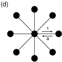
Figure 1: (a) Complete graph, (b) undirected cycle, (c) directed cycle, and (d) weighted star.

Consider the evolutionary dynamics on the complete graph of $N$ nodes depicted in Fig. 1(a). Self loops are excluded. The complete graph is undirected and regular, where a regular graph is one in which the indegree and the outdegree of all the nodes are the same. For undirected regular graphs, BD-B, DB-D, and LD are all equivalent to the Moran process with the same population size $N$ [Antal et al., 2006, Sood et al., 2008]. Therefore, $F(r)$ is given by Eq. (1). For BD-D, we obtain

$$F(r)=\frac{1}{1+(N-1)\sum^{N-1}_{m=1}\frac{r^{-m+1}}{m+r(N-1-m)}}.$$ (3)

For DB-B, we obtain

$$F(r)=\frac{N-1}{N}\frac{1-r^{-1}}{1-r^{-N+1}}.$$ (4)

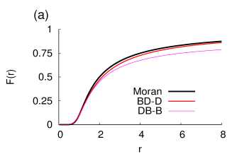
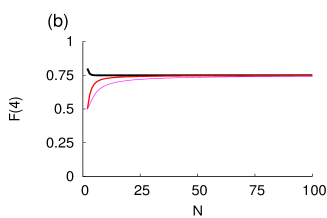
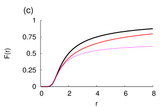
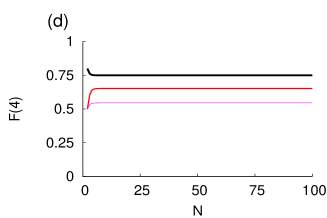
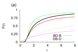
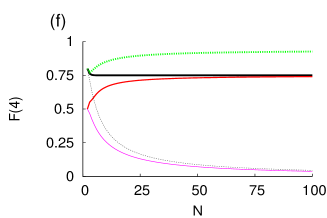
Figure 2: (Color online) Fixation probability for (a, b) the complete graph, (c, d) the undirected cycle, and (e, f) the star, under different update rules. We set $N=10$ and vary $r$ in (a, c, e). We set $r=4$ and vary $N$ in (b, d, f). Thick solid black lines, medium solid red lines, and thin solid magenta lines correspond to the standard Moran process, BD-D, and DB-B, respectively. In (e, f), thick dashed green lines and thin dashed gray lines correspond to BD-B and DB-D, respectively.

In Fig. 2(a), $F(r)$ for the Moran process, BD-D, and DB-B is compared for the complete graph with $N=10$. The three lines cross at neutrality, that is, $(r,F(r))=(1,1/N)$. The complete graph is an evolutionary suppressor under BD-D, even though $\lim_{r\to\infty}F(r)=1$ and $\lim_{r\to 0}F(r)=0$. This is because selection occurs among the $N-1$ nodes excluding the reproducing node. DB-B is a stronger suppressor than BD-D. Differently from BD-D, we obtain $\lim_{r\to\infty}F(r)=(N-1)/N$ and $\lim_{r\to 0}F(r)=0$ for DB-B, so that a mutant may not fix under DB-B even if its fitness is infinitely large.

For the three different cases, $F(4)$ is plotted against $N(\geq 2)$ in Fig. 2(b). The fixation probability for BD-D and DB-B converges to that for the Moran process as $N\to\infty$. Remarkably, for BD-D and DB-B, the existence of more competitors in the population, that is, larger $N$, leads to the higher fixation probability of the single type-$A$ mutant. As $N$ increases, selection acts on more nodes relative to the population size (i.e., $(N-1)/N$) under BD-D and DB-B. Then type-$A$ nodes, which are rare in an early stage of dynamics, are involved in competition for survival (under BD-D) or reproduction (under DB-B) more often such that type $A$ takes advantage of being inherently fitter than type $B$.

4.2 Undirected cycle

Consider the undirected cycle of size $N$ depicted in Fig. 1(b). Because the undirected cycle is unweighted and regular, BD-B, DB-D, and LD are again equivalent to the Moran process, and $F(r)$ is given by Eq. (1). For BD-D, we obtain

$$F(r)=\frac{1-r^{-1}}{1+\frac{r-1}{r(r+1)}+\frac{(r^{2}-2r-1)r^{-N+1}}{r+1}}.$$ (5)

For DB-B, we obtain

$$F(r)=\frac{1-r^{-1}}{1+\frac{r-1}{2r}+\frac{(r-3)r^{-N+1}}{2}}.$$ (6)

For the undirected cycle, $F(r)$ with $N=10$ and $F(4)$ with $N$ varied are shown in Fig. 2(c) and Fig. 2(d), respectively. Qualitatively agreeing with the case of the complete graph, BD-D is suppressing, and DB-B is even more so. In contrast to the case of the complete graph, BD-D and DB-B persist to be suppressing for large $N$. Under BD-D and DB-B, selection operates on about $\left<k\right>$ individuals, where $\left<k\right>$ is the mean degree of the network, whereas selection operates on $N$ individuals under BD-B, DB-D, and LD. For the complete graph, the difference diminishes as $N\to\infty$ because $\left<k\right>=N-1$. For the undirected cycle, $\left<k\right>=2$ independent of $N$, which is a likely reason why BD-D and DB-B are suppressing even for large $N$.

4.3 Directed cycle

Consider the directed cycle of size $N$ depicted in Fig. 1(c). It is straightforward to verify that the evolutionary dynamics under BD-B, DB-D, and LD are equivalent to the Moran process. For BD-D and DB-B, selection pressure is totally annihilated, that is, $F(r)=1/N$.

4.4 Star

Consider the star with $N$ nodes depicted in Fig. 1(d). One central hub is connected to the other $N-1$ leaves. Only in this section, we introduce the edge weight for a computation purpose. Specifically, each edge outgoing from the hub has weight $1$, and each edge incoming to the hub has weight $a$. The edge weight is assumed to be multiplied to the likelihood with which the edge is used for reproduction (see Secs. 2.2-2.6 and Appendix B).

The fixation probability for the weighted star under LD is given by

$$F(r)=\frac{1-\frac{N-1}{N}\frac{r+a}{r(ra+1)}-\frac{1}{N}\frac{ra+1}{r(r+a)}}{1-r^{-N}\left(\frac{r+a}{ra+1}\right)^{N-2}}.$$ (7)

For general $a$, we obtain in the limit $N\to\infty$

$$K=-\frac{\ln\frac{r+a}{r(ra+1)}}{\ln r},$$ (8)

where $K$ is defined by Eq. (2). Although in an incomplete form of Eq. (8), which includes $r$ in the RHS, $K>1$ ($K<1$) for all $r\neq 1$ when $a>1$ ($a<1$). Therefore, the weighted star is an amplifier (a suppressor) when $a>1$ ($a<1$). With $a=1$ in Eq. (7), $F(r)$ is equal to Eq. (1). This is expected because the evolutionary dynamics for any undirected network are equivalent to the Moran process under LD [Antal et al., 2006, Sood et al., 2008].

As shown in Appendix B, LD on the weighted star with $a=N-1$ is equivalent to BD-B on the unweighted star. Therefore, the unweighted star is an amplifier under BD-B. Particularly, in the limit $N\to\infty$, Eq. (7) yields $K=2$, consistent with the previous result [Lieberman et al., 2005]. The theory for undirected uncorrelated networks [Antal et al., 2006, Sood et al., 2008] also predicts $K=\left<k\right>\left<k^{-1}\right>\approx 2$ for the undirected star under BD-B.

Also shown in Appendix B is that LD on the weighted star with $a=1/(N-1)$ is equivalent to DB-D on the unweighted star. Setting $a=1/(N-1)$ in Eq. (8) yields $K=0$ in the limit $N\to\infty$. This is consistent with the result for undirected uncorrelated networks: $K=\left<k\right>^{2}/\left<k^{2}\right>=2/N$ [Antal et al., 2006, Sood et al., 2008].

The fixation probability for BD-D is given by

$$F(r)=\frac{(N-1)N\frac{1+r(N-2)}{2+r(N-2)}+1}{N}\frac{1}{1+\frac{1+r(N-1)}{r-1}\left(1-\frac{r^{-N+2}N}{N-1+r}\right)},$$ (9)

and that for DB-B is given by

$$F(r)=\frac{(rN+N+2r-2)(rN-r+1)}{N^{2}(N+2r-2)(r+1)}.$$ (10)

For the unweighted star, $F(r)$ with $N=10$ and $F(4)$ with $N$ varied are shown in Fig. 2(e) and Fig. 2(f), respectively. LD corresponds to the Moran process, and BD-B is the only amplifying update rule. Among the other three suppressing update rules, DB-B is the most suppressing. Figure 2(f) indicates that BD-D is more suppressing than DB-B for small $N$ and vice versa for large $N$. As $N$ tends large, DB-B and DB-D become strongly suppressing. Indeed, both Eq. (7) with $a=1/(N-1)$ representing DB-D and Eq. (10) representing DB-B yield $F(r)=O(1/N)$, $r>1$. In contrast, the fixation probability for BD-D approaches that for the Moran process as $N\to\infty$; Eq. (9) yields $\lim_{N\to\infty}F(r)=(r-1)/r$, which agrees with the result for the Moran process derived from Eq. (1).

5 Numerical results

Here we report numerical results for the fixation probability of the mutant type with $r=4$. Equation (1) implies $\lim_{N\to\infty}F(r)=3/4$ for the Moran process. If $F(4)$ measured for a combination of a network and an update rule is larger (smaller) than $3/4$, that combination is probably amplifying (suppressing). Whether the combination is amplifying or suppressing and to what extent actually depend on $r$. However, our extensive numerical results suggest that this dependence is not strong unless $r$ is extremely small or large. The values of $F(4)$ are also well correlated with $dF(r)/dr|_{r=1}$, which is the sensitivity of the selection pressure at neutrality. Therefore, we assume $r=4$ in the following.

A graph $G$ is called strongly connected if there is a directed path from an arbitrary chosen node to another. For $G$ that is not strongly connected, the mutant type introduced at a node in a downstream component never fixates, and the fixation problem is ascribed to that for the most upstream strongly connected component of $G$ [Lieberman et al., 2005]. Therefore, we assume that $G$ is strongly connected without loss of generality.

5.1 Small networks

In this section, we present numerical results for small networks. The evolutionary dynamics are interpreted as a discrete-time Markov chain on a finite space. A state of the Markov chain is specified by an assignment of type $A$ or $B$ to each node, so that there are $2^{N}$ possible states. Among them, the two states corresponding to the unanimity of $A$ and that of $B$ are the unique absorbing states. Given $G$ and an update rule, we obtain the exact fixation probability by solving a system of linear equations of $2^{N}-2$ variables (see Appendix A for methods). Because of the computation time, we set $N=6$ and calculate $F(4)$ for all the 1047008 strongly connected networks under the five update rules. The results are qualitatively similar for $N=4$ and $N=5$ (data not shown).

To visualize the results and to correlate $F(4)$ with the structure of $G$, we regard the values of $F(4)$ for different networks as different data points. Then we regress $F(4)$ of these data points against various measurements of the network, which we call order parameters. We look for the order parameters that are more correlated with $F(4)$ than other order parameters. Our choice of the order parameters is arbitrary. For each of the five update rules, we list in Tab. 1 the Pearson correlation coefficient between $F(4)$ and the order parameters, where $\left<\cdot\right>$ denotes the average over the nodes. The first order parameter is the mean degree $\left<k\right>\equiv\left<k^{in}\right>=\left<k^{out}\right>$, where $k^{in}$ and $k^{out}$ is the indegree and the outdegree of a node, respectively. Seven order parameters are normalized moments of the degree distribution: $\left<k\right>\left<1/k^{in}\right>$, $\left<k\right>\left<1/k^{out}\right>$, $\left<k\right>^{2}/\left<\left(k^{in}\right)^{2}\right>$, $\left<k\right>^{2}/\left<\left(k^{out}\right)^{2}\right>$, $\left<k\right>^{2}/\left<k^{in}k^{out}\right>$, $\left<k^{out}/k^{in}\right>$, and $\left<k^{in}/k^{out}\right>$. The other two order parameters are the normalized standard deviation of the node temperature: $std(T^{in})$ and $std(T^{out})$. The temperature $T^{in}_{i}$ of node $v_{i}$ [Lieberman et al., 2005] is defined by $T^{in}_{i}\equiv\sum_{j;(v_{j},v_{i})\in E}\left(w_{ji}/\sum_{l}w_{jl}\right)$. We define $std(T^{in})\equiv$ $\sqrt{\sum_{i=1}^{N}\left(T^{in}_{i}-\left<T^{in}\right>\right)^{2}/N}/\left<T^{in}\right>$ $=\sqrt{\sum_{i=1}^{N}\left(T^{in}_{i}-1\right)^{2}/N}$, where we have used $\left<T^{in}\right>=1$. For isothermal networks, which satisfy $std(T^{in})=0$, the evolutionary dynamics under BD-B are equivalent to the Moran process [Lieberman et al., 2005]. Similarly, we define the temperature for the outdegree by $T^{out}_{i}\equiv\sum_{j;(v_{i},v_{j})\in E}\left(w_{ij}/\sum_{l}w_{lj}\right)$, which satisfies $\left<T^{out}\right>=1$, and measure $std(T^{out})$.

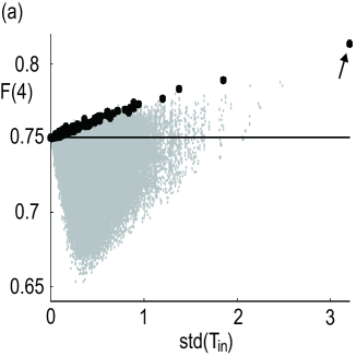
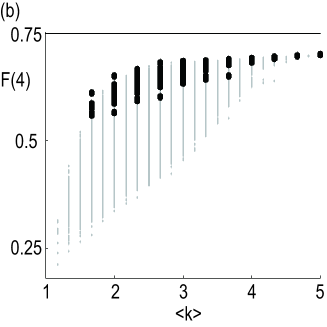
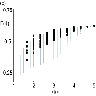
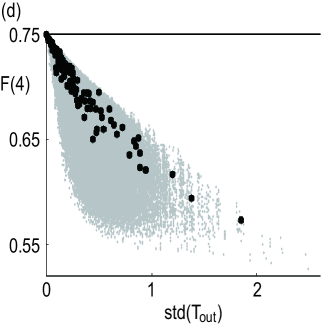
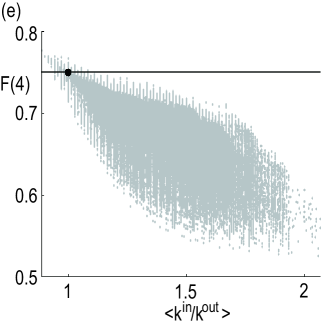
Figure 3: Fixation probability $F(4)$ for the strongly connected networks (gray dots) and for the undirected networks (black circles) of size $N=6$. The line $F(4)=0.7502$ corresponds to the Moran process. (a) BD-B versus $std(T^{in})$, (b) BD-D versus $\left<k\right>$, (c) DB-B versus $\left<k\right>$, (d) DB-D versus $std(T^{out})$, and (e) LD versus $\left<k^{in}/k^{out}\right>$.

Under BD-B, we have not found an order parameter that is strongly correlated with $F(4)$, as listed in Tab. 1. For a visualization purpose, we plot $F(4)$ against $std(T_{in})$ for all the networks in Fig. 3(a). Each gray dot in the figure corresponds to a network of size $N=6$. Black circles are for undirected networks. The Moran process with $N=6$ yields $F(4)=0.7502$, which is shown by the solid line. Because $r=4>1$, networks with $F(4)$ above (below) the solid line are amplifiers (suppressors). Figure 3(a) suggests the following. First, the undirected star (indicated by the arrow) is by far the most amplifying among all the networks. Most networks that yield large $F(4)$ are variants of the star and have large $std(T_{in})$. Second, all the undirected networks are amplifiers under BD-B, consistent with the result that $F(r)$ for undirected uncorrelated networks is given by Eq. (2) with $K=\left<k\right>\left<k^{-1}\right>>1$ [Antal et al., 2006, Sood et al., 2008]. Indeed, $F(4)$ for undirected networks with $N=6$ (black circles) are strongly correlated with $\left<k\right>\left<k^{-1}\right>$ (data not shown). Third, a majority of directed networks is suppressor. The mean and the standard deviation of $F(4)$ based on all the networks and those based on the undirected networks compared in Tab. 2 indicate a significant difference.

Under BD-D, $\left<k\right>$ is most strongly correlated with $F(4)$. The values of $F(4)$ for different networks are plotted against $\left<k\right>$ in Fig. 3(b). The complete graph, which corresponds to $\left<k\right>=N-1=5$, is the least suppressing, although it is nevertheless a suppressor, as shown in Sec. 4.1. All the networks are suppressors. Table 2 indicates that the suppression is generally stronger under BD-D than under BD-B and that directed networks are stronger suppressors than undirected networks on an average.

Under DB-B also, $\left<k\right>$ is most strongly correlated with $F(4)$. Figure 3(c), which shows the relation between $F(4)$ and $\left<k\right>$, indicates that the complete graph achieves the largest $F(4)$, that all the networks are suppressors, and that directed networks are more suppressing than undirected networks on an average. These tendencies are similar to those for BD-D.

Under DB-D, $std(T^{out})$ is most strongly correlated with $F(4)$. Equation (2) with $K=\left<k\right>^{2}/\left<k^{2}\right>$, which was derived for undirected uncorrelated networks [Antal et al., 2006, Sood et al., 2008], approximates our numerical results for the undirected networks (data not shown). However, $std(T^{out})$ seems to be a better predictor of $F(4)$ than $\left<k\right>^{2}/\left<\left(k^{in}\right)^{2}\right>$, $\left<k\right>^{2}/\left<\left(k^{out}\right)^{2}\right>$, and $\left<k\right>^{2}/\left<k^{in}k^{out}\right>$, probably because of the small network size. Figure 3(d) indicates that $F(4)$ for the networks with $std(T^{out})=0$ is equal to $F(4)$ for the Moran process, that all the other networks are suppressors, and that directed networks are more suppressing than undirected networks on average.

Under LD, $\left<k^{in}/k^{out}\right>$ is most strongly correlated with $F(4)$. Evolutionary dynamics for undirected networks are equivalent to the Moran process [Antal et al., 2006, Sood et al., 2008]. Figure 3(e) indicates that directed networks are generally more suppressing than undirected networks, that there are both amplifiers and suppressors among directed networks with the majority being suppressors, and that smaller $\left<k^{in}/k^{out}\right>$ tends to yield larger $F(4)$.

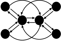
Figure 4: The network with $N=6$ that yields the largest $F(4)$ under LD.

The network that achieves the largest $F(4)$ is shown in Fig. 4. Most networks that produce large $F(4)$ are variants of this network. Because $\sum_{i=1}^{N}k_{i}^{in}=\sum_{i=1}^{N}k_{i}^{out}$, a small value of $\left<k^{in}/k^{out}\right>$ requires that $k^{in}<k^{out}$ holds for many small-degree nodes and that $k^{in}>k^{out}$ holds for a relatively small number of hubs. The network shown in Fig. 4 complies with this property. In Fig. 4, each of the two hubs links to the half of the peripheral nodes, whereas each peripheral node links to both hubs. If we merge the two hubs into one as an approximation, the network is regarded as a weighted star with $a=2$ (Fig. 1(d)). The weighted star with $a=2$ is indeed an amplifier, as shown in Sec. 4.4.

Based on the numerical results for the five update rules, we claim the following. First, directed networks tend to be suppressors compared to undirected networks regardless of the update rule. Second, some update rules (i.e., BD-D, DB-B, and DB-D) are much more suppressing than the others (i.e., BD-B and LD). Particularly, the magnitude of the amplification is ordered as: BD-B $>$ LD $>$ DB-D $>$ BD-D $>$ DB-B (Tab. 2), which is consistent with the one for the undirected star with small $N$ (Fig. 2(f)). In a single time step, the selection pressure operates on $N$ nodes for BD-B, DB-D, and LD. However, it operates on at most $N-1$ nodes for BD-D and DB-B, because the node first selected for reproduction under BD-D or for death under DB-B does not participate in the competition. This is a main reason why BD-D and DB-B are strongly suppressing. We will corroborate these points by numerical simulations of large networks in Sec. 5.2.

5.2 Large networks

Because of the computational cost, the exact numerical analysis performed in Sec. 5.1 is feasible only for small networks. In this section, we examine evolutionary dynamics on larger networks by Monte Carlo simulations.

We use the Erdös–Rényi (ER) random graph, SF networks, and their directed versions of different sizes (e.g. Albert and Barabási, 2002; Newman, 2003). We generate the undirected ER graph of mean degree $\left<k\right>$ by connecting each pair of nodes with probability $\left<k\right>/(N-1)$. The directed ER graph is generated by connecting each ordered pair of nodes with probability $2\left<k\right>/(N-1)$ so that $\left<k^{in}\right>=\left<k^{out}\right>=\left<k\right>$. In both cases, the degree distribution $p(k)$ follows a poisson distribution with mean $\left<k\right>$: $p(k)\approx e^{-k/\left<k\right>}/\left<k\right>$. For SF networks, we assume $p(k)\propto k^{-3}$, ($\left<k\right>/2\leq k$), where the power-law exponent $3$ is an arbitrary choice. The SF network represents the situation in which the degree is strongly heterogeneous [Albert and Barabási, 2002, Newman, 2003]. To generate a SF network, we first determine the degree of each node stochastically according to the power-law distribution $p(k)$ with the restriction that the sum of the degree is even. Then, we randomly add edges one by one so that the predetermined degrees are respected at each node [Albert and Barabási, 2002, Newman, 2003]. For undirected and directed SF networks, the added edges are undirected and directed, respectively. In each of the four network models, we discard networks that are not strongly connected.

To calculate $F(4)$, we perform 2000 runs for each initial location of the type $A$ individual and count the fraction of the $2000N$ runs in which the unanimity of type $A$ is reached. This is a Monte Carlo realization of the fixation probability. For a fixed $N$, $\left<k\right>$, network model, and update rule, we calculate the average and the standard deviation of $F(4)$ based on 20 samples of networks.

For $\left<k\right>=10$, $F(4)$ under BD-B is plotted against $N$ for the ER and SF networks in Figs. 5(a) and (b), respectively. The standard deviation is shown by the error bars. The SF networks are more amplifying than the ER networks, consistent with the previous results [Lieberman et al., 2005, Antal et al., 2006, Sood et al., 2008]. In addition, undirected networks (solid lines) are more amplifying than directed networks (dashed lines), even for large $N$. The same tendencies are found for BD-D (Figs. 5(c) and (d)), DB-B (Figs. 5(e) and (f)), DB-D (Figs. 5(g) and (h)), and LD (Figs. 5(i) and (j)). This is a strong indication that directionality of edges generally suppresses the selection pressure.

For each of the four types of networks used in Fig. 5, the strength of the selection pressure is ordered as: BD-B $>$ BD-D, LD $>$ DB-D $>$ DB-B. This order is consistent with the one for the unweighted star with large $N$ (Fig. 2(f)). Compared to the results for the small networks shown in Sec. 5.1, BD-D is much less suppressing in large networks, as shown in Figs. 5(c) and (d). This is a bit surprising because we have kept $\left<k\right>=10$ in Fig. 5 so that the competition for survival happens among roughly $\left<k\right>\ll N$ nodes per unit time. In contrast, DB-B remains strongly suppressing even for large $N$ (Figs. 5(e) and (f)). An increase in $\left<k\right>$ with $N$ fixed makes DB-B less suppressing, as shown in Fig. 6. This is consistent with the behavior of the ensemble of the small networks (Fig. 3(c)).

6 A theoretical explanation of the effect of directionality

The finding that the directionality of the network suppresses the selection pressure can be explained for LD on a simple network. Consider a bidirectionally but asymmetrically connected two-node network. Edge ($v_{1}$, $v_{2}$) (from $v_{1}$ to $v_{2}$) has weight unity, and edge ($v_{2}$, $v_{1}$) has weight $a$. Even though we have formulated the evolutionary dynamics on unweighted networks, the extension to the case of weighted networks is straightforward (also refer to the analysis of the weighted star in Appendix B). By enumerating the possible reproduction events per unit time, we obtain

$$F(AB) =\frac{rF(AA)+aF(BB)}{r+a} =\frac{r}{r+a},$$ (11)

$$F(BA) =\frac{raF(AA)+F(BB)}{ra+1} =\frac{ra}{ra+1},$$ (12)

where the first and the second arguments of $F$ are the types at $v_{1}$ and $v_{2}$, respectively, and $F$ is the fixation probability starting from that network state. Note that $F(AA)=1$ and $F(BB)=0$. Using Eqs.  (11) and (12), we obtain

$$F(r)=\frac{F(AB)+F(BA)}{2}=\frac{1}{2}\left(\frac{r}{r+a}+\frac{ra}{ra+1}\right).$$ (13)

For $r>1$, $F(r)$ as a function of $a$ takes the maximum at $a=1$. For $r<1$, $F(r)$ takes the minimum at $a=1$. Therefore, the unweighted network (i.e., $a=1$) is the most amplifying when we vary $a$. LD on this unweighted network (i.e., $a=1$) is equivalent to the Moran process with $N=2$. Accordingly, weighted networks (i.e., $a\neq 1$) are suppressors, and the suppression is stronger as $a$ deviates from unity.

The applicability of the arguments above is beyond the two-node network. Suppose that a network is divided into two modules with homogeneous intramodular connectivity and that intermodular connectivity is sparse and homogeneous, possibly with more edges from one module to the other than the converse. Then the fixation probability of a mutant on a particular node will depend only on the module in which the initial mutant invades. In this case, we can approximate the network by the two-node weighted network, where the edge weights between the two aggregated nodes represent the gross connectivity between the two modules.

7 Discussion

Motivated by the observation that many real ecological and social networks underlying reproduction in evolutionary dynamics are directed or weighted, we have investigated the fixation probability on networks with directed edges under five update rules. For undirected networks, selection pressure relies on the network and the update rule, which reproduces the previous results [Lieberman et al., 2005, Antal et al., 2006, Sood et al., 2008]. Our main conclusions in the present paper are twofold.

First, directionality of edges suppresses the selection pressure for all the network types and the update rules that we have dealt with. We have presented numerical evidence for different sizes of networks (Sec. 5) and simple analytical arguments (Sec. 6) to support this claim. Note that many ecological and social situations in which evolutionary dynamics take place can be modeled as directed or weighted networks rather than undirected and unweighted networks. Spreads of a type from one habitat to another may be easier than in the other direction because of heterogeneity in habitats and other geographical factors (see Sec. 1 for references). Accordingly, fixation in real contact networks may be less controlled by the values of fitness than in the corresponding undirected networks or well-mixed populations.

Second, the strength of the selection pressure depends on the update rule for various networks, no matter whether edges are directed or not (Secs. 4 and 5). This conclusion extends the previous findings [Antal et al., 2006, Sood et al., 2008]. For BD-D, DB-B, and DB-D, no evolutionary amplifier has been found by our exhaustive numerical analysis for small $N$ (Sec. 5.1). Moreover, DB-B is strongly suppressing compared to the other update rules. In evolutionary game theory, DB-B [Nakamaru et al., 1998, Ohtsuki et al., 2006, Ohtsuki and Nowak, 2006] and its variants [Nowak and May, 1992, Santos and Pacheco, 2005] have commonly been used. In games, the fitness of a type is not constant, as assumed in the present paper, but depends on neighbors’ types. Therefore, the results obtained in this work are not immediately applicable to evolutionary games. However, these previous results on evolutionary games might considerably change under update rules less suppressing than DB-B, as has been argued [Nakamaru et al., 1998, Ohtsuki et al., 2006, Ohtsuki and Nowak, 2006].

We have treated directed but unweighted networks for the sake of clarity of the analysis. However, we believe that our conclusions for directed networks extend to the case of weighted networks. This is partly supported by the analysis of the two-node weighted network presented in Sec. 6. In addition, if we quantize the edge weight and allow multiple directed edges between two nodes, a weighted network can be regarded as a directed unweighted network.

A unique point in our analysis is the use of very small networks with $N=6$. Small networks per se appear in many ecological contexts. For example, the number of relevant habitats may not be very large [Gustafson and Gardner, 1996, Tischendorf and Fahrig, 2000, Schick and Lindley, 2007]. In addition, small directed networks are likely to be structural and functional building blocks of large networks [Milo et al., 2002, Itzkovitz et al., 2003]. According to the present analysis, the effect of the directionality of edges and that of the update rule are mostly consistent between small and large networks. We believe that the conclusions of the present paper apply to real evolutionary dynamics in populations of various scales.

Appendix A: Numerical procedure for small networks

Here, we explain the methods for exactly calculating the fixation probability for strongly connected networks. Because each node takes either type $A$ or $B$, there are $2^{N}$ possible states of the evolutionary dynamics. We define the fixation probability for a state, which may have multiple type-$A$ nodes, by the probability that type $A$ fixates starting from that state. The fixation probability for the all-$A$ state is 1, and that for the all-$B$ state is 0.

Given a network, an update rule, and $r$, the evolutionary dynamics are equivalent to a nearest-neighbor random walk on the $N$-dimensional hypercube comprising $2^{N}$ points. In each time step, the type at a node replaces the type at one of its neighbors in the original evolutionary dynamics. Therefore, at most one node flips its type per unit time. In terms of the random walk on the hypercube, the walker moves to a neighboring state or does not move. The random walk continues until either the all-$A$ state or the all-$B$ state is reached.

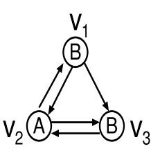
Figure 7: A directed network with $N=3$.

Consider an example network shown in Fig. 7. Denote the fixation probability for the state shown in Fig. 7 by $F(BAB)$, where the first, second, and the third arguments ($A$ or $B$) correspond to the types at $v_{1}$, $v_{2}$, and $v_{3}$, respectively. In a unit time, state $BAB$ may change to $AAB$, $BBB$, or $BAA$. Otherwise, it does not change. Under BD-B, for example, the fixation probability satisfies

$$F(BAB)=\frac{1}{r+2}\frac{F(BBB)+F(BAB)}{2}+\frac{r}{r+2}\frac{F(AAB)+F(BAA)}{2}+\frac{1}{r+2}F(BBB).$$ (14)

The first, second, and third terms in the RHS of Eq. (14) represent the propagation of the type at $v_{1}$, $v_{2}$, and $v_{3}$ to its neighbor, respectively. Noting the boundary conditions $F(BBB)=0$ and $F(AAA)=1$, we can write down the other five linear equations corresponding to the single-step transition of $F(ABB)$, $F(BBA)$, $F(AAB)$, $F(ABA)$, and $F(BAA)$. The fixation probabilities are obtained by solving the system of the six linear equations. The fixation probability starting from a single type-$A$ node is given by $F(r)=\left[F\left(ABB\right)+F\left(BAB\right)+F\left(BBA\right)\right]/3$. Generally speaking, the fixation probability for an $N$-node network is obtained by solving a system of $2^{N}-2$ linear equations. A standard method such as the Gauss elimination requires $O\left(\left(2^{N}\right)^{3}\right)$ time of computation.

For small $N$, we can enumerate all the possible networks [Milo et al., 2002, Itzkovitz et al., 2003]. There are 1047008 strongly connected directed networks out of 1530843 weakly connected directed networks with $N=6$. We cannot solve the fixation probability for $N>6$ due to the computational cost of enumerating the directed networks, but not due to the cost of solving systems of $2^{N}-2$ linear equations.

Appendix B: Fixation probability for simple graphs

In this appendix, we show detailed calculations of the fixation probability for simple graphs. Following a standard procedure, we map the evolutionary dynamics onto the discrete-time nearest-neighbor random walk on interval $\{0,1,2,\ldots,N\}$. The position on the interval corresponds to the number of type-$A$ individuals in a network of size $N$. Positions 0 and $N$ are the only absorbing states. The type-$A$ individuals increase or decrease at most by one per unit time. The probability $F_{m}$ that the walker at position $m$ eventually reaches position $N$ satisfies the following relations:

$$F_{0} = 0,$$ (15)

$$F_{m} = \alpha_{m}F_{m+1}+(1-\alpha_{m}-\beta_{m})F_{m}+\beta_{m}F_{m-1},\quad(1\leq m\leq N-1)$$ (16)

$$F_{N} = 1,$$ (17)

for some $\alpha_{m}$ and $\beta_{m}$ ($1\leq m\leq N-1$). Then, the fixation probability for a single mutant is represented by [Moran, 1958, Ewens, 2004, Nowak, 2006]:

$$F_{1}=\frac{1}{1+\sum^{N-1}_{m=1}\prod^{m}_{m^{\prime}=1}\frac{\beta_{m^{\prime}}}{\alpha_{m^{\prime}}}}.$$ (18)

Complete graph

Consider the complete graph with $N$ nodes. The evolutionary dynamics under BD-B are equivalent to the Moran process, and Eq. (16) becomes

$$F_{m}=\frac{mr\frac{(N-m)F_{m+1}+(m-1)F_{m}}{N-1}+(N-m)\frac{(N-m-1)F_{m}+mF_{m-1}}{N-1}}{mr+N-m}.$$ (19)

Therefore, $\alpha_{m}=mr(N-m)/[(mr+N-m)(N-1)]$, $\beta_{m}=m(N-m)/[(mr+N-m)(N-1)]$, and $\beta_{m}/\alpha_{m}=1/r$, which plugged into Eq. (18) leads to Eq. (1). DB-D and LD also yield $\beta_{m}/\alpha_{m}=1/r$ and hence the same result as that for BD-B.

For BD-D, we obtain

$$F_{m}=\frac{m}{N}\frac{(N-m)F_{m+1}+\frac{m-1}{r}F_{m}}{\frac{m-1}{r}+N-m}+\frac{N-m}{N}\frac{(N-1-m)F_{m}+\frac{m}{r}F_{m-1}}{\frac{m}{r}+N-1-m}.$$ (20)

Therefore,

$$\frac{\beta_{m}}{\alpha_{m}}=\frac{m-1+r(N-m)}{r\left[m+r\left(N-1-m\right)\right]}.$$ (21)

Plugging Eq. (21) into Eq. (18) leads to Eq. (3).

For DB-B, we obtain

$$F_{m}=\frac{m}{N}\frac{r(m-1)F_{m}+(N-m)F_{m-1}}{r(m-1)+N-m}+\frac{N-m}{N}\frac{rmF_{m+1}+(N-1-m)F_{m}}{rm+N-1-m}.$$ (22)

Therefore,

$$\frac{\beta_{m}}{\alpha_{m}}=\frac{rm+N-1-m}{r\left[r(m-1)+N-m\right]}.$$ (23)

Plugging Eq. (23) into Eq. (18) leads to Eq. (4).

Undirected cycle

Consider the undirected cycle with $N$ nodes. Under BD-D, we obtain

$$F_{1} = \frac{1}{N}F_{2}+\frac{2}{N}\frac{F_{1}+\frac{F_{0}}{r}}{1+\frac{1}{r}}+\frac{N-3}{N}F_{1},$$ (24)

$$F_{m} = \frac{2}{N}\frac{F_{m+1}+\frac{F_{m}}{r}}{1+\frac{1}{r}}+\frac{2}{N}\frac{F_{m}+\frac{F_{m-1}}{r}}{1+\frac{1}{r}}+\frac{N-4}{N}F_{m},\quad(2\leq m\leq N-2)$$ (25)

$$F_{N-1} = \frac{2}{N}\frac{F_{N}+\frac{F_{N-1}}{r}}{1+\frac{1}{r}}+\frac{1}{N}F_{N-2}+\frac{N-3}{N}F_{N-1}.$$ (26)

Therefore,

$$\frac{\beta_{m}}{\alpha_{m}}=\left\{\begin{array}[]{ll}\frac{2}{r+1},&(m=1)\\ \frac{1}{r},&(2\leq m\leq N-2)\\ \frac{r+1}{2r}.&(m=N-1)\end{array}\right.$$ (27)

Plugging Eq. (27) into Eq. (18) leads to Eq. (5).

Under DB-B, we obtain

$$F_{1} = \frac{2}{N}\frac{rF_{2}+F_{1}}{r+1}+\frac{1}{N}F_{0}+\frac{N-3}{N}F_{1},$$ (28)

$$F_{m} = \frac{2}{N}\frac{rF_{m+1}+F_{m}}{r+1}+\frac{2}{N}\frac{rF_{m}+F_{m-1}}{r+1}+\frac{N-4}{N}F_{m},\quad(2\leq m\leq N-2)$$ (29)

$$F_{N-1} = \frac{1}{N}F_{N}+\frac{2}{N}\frac{rF_{N-1}+F_{N-2}}{r+1}+\frac{N-3}{N}F_{N-1}.$$ (30)

Therefore,

$$\frac{\beta_{m}}{\alpha_{m}}=\left\{\begin{array}[]{ll}\frac{r+1}{2r},&(m=1)\\ \frac{1}{r},&(2\leq m\leq N-2)\\ \frac{2}{r+1}.&(m=N-1)\end{array}\right.$$ (31)

Plugging Eq. (31) into Eq. (18) leads to Eq. (6).

Star

Consider the undirected star with $N$ nodes. To calculate the fixation probability for BD-B and LD simultaneously, it is convenient to introduce the edge weight. We assume that an edge from the hub to a leaf is endowed with weight unity and one from a leaf to the hub is endowed with weight $a$ (Fig. 1(d)). The edge weight works as a multiplicative factor to the probability that this edge is chosen for reproduction, which is explained in Sec. 2. Denote by $F_{m,A}$ ($F_{m,B}$) ($0\leq m\leq N-1$) the fixation probability of type $A$ when there are $m$ type-$A$ leaves and the hub is occupied by type $A$ ($B$).

BD-B for the unweighted star is equivalent to LD with selection on the birth, which is actually the ordinary LD, for the weighted star with $a=N-1$. DB-D for the unweighted star is equivalent to LD with selection on the death, which is again the ordinary LD, for the weighted star with $a=1/(N-1)$. Therefore, we calculate the fixation probability for the weighted star under LD. Interpreting LD as the LD with selection on the birth, we obtain

$$F_{m,A} = \frac{rmaF_{m,A}+(N-1-m)aF_{m,B}+rmF_{m,A}+r(N-1-m)F_{m+1,A}}{rma+(N-1-m)a+r(N-1)},$$

$$(0\leq m\leq N-2)$$

$$F_{m,B} = \frac{rmaF_{m,A}+(N-1-m)aF_{m,B}+mF_{m-1,B}+(N-1-m)F_{m,B}}{rma+(N-1-m)a+(N-1)}.$$

$$(1\leq m\leq N-1)$$

Eqs. (Star) and (Star), respectively, lead to

$$(r+a)F_{m,A} =aF_{m,B}+rF_{m+1,A}, (0\leq m\leq N-2)$$ (34)

$$(ra+1)F_{m,B} =raF_{m,A}+F_{m-1,B}. (1\leq m\leq N-1)$$ (35)

By combining Eqs. (34) and (35), we obtain

$$(r^{2}a+2r+a)F_{m,A}-r(ra+1)F_{m+1,A}-(r+a)F_{m-1,A}=0.\quad(1\leq m\leq N-2)$$ (36)

The solution to Eq. (36) that satisfies $(r+a)F_{0,A}=rF_{1,A}$, which comes from Eq. (34) with $m=0$ and $F_{0,B}=0$, and $F_{N-1,A}=1$ is

$$F_{m,A}=\frac{\frac{r(r+a)}{ra+1}-\left(\frac{r+a}{r(ra+1)}\right)^{m}}{\frac{r(r+a)}{ra+1}-\left(\frac{r+a}{r(ra+1)}\right)^{N-1}}.$$ (37)

Plugging Eq. (37) into Eq. (34) leads to

$$F_{m,B}=\frac{\frac{r(r+a)}{ra+1}\left[1-\left(\frac{r+a}{r(ra+1)}\right)^{m}\right]}{\frac{r(r+a)}{ra+1}-\left(\frac{r+a}{r(ra+1)}\right)^{N-1}}.$$ (38)

The fixation probability for a single mutant is represented by

$$F(r)=\frac{(N-1)F_{1,B}+F_{0,A}}{N}=\frac{1-\frac{N-1}{N}\frac{r+a}{r(ra+1)}-\frac{1}{N}\frac{ra+1}{r(r+a)}}{1-r^{-N}\left(\frac{r+a}{ra+1}\right)^{N-2}}.$$ (39)

For BD-D on the unweighted star, we obtain

$$F_{m,A} = \frac{\frac{\frac{m}{r}}{\frac{m}{r}+N-1-m}F_{m,A}+\frac{N-1-m}{\frac{m}{r}+N-1-m}F_{m+1,A}+mF_{m,A}+(N-1-m)F_{m,B}}{N},$$

$$(0\leq m\leq N-2)$$

$$F_{m,B} = \frac{\frac{\frac{m}{r}}{\frac{m}{r}+N-1-m}F_{m-1,B}+\frac{N-1-m}{\frac{m}{r}+N-1-m}F_{m,B}+mF_{m,A}+(N-1-m)F_{m,B}}{N}.$$

$$(1\leq m\leq N-1)$$

Equations (Star) and (Star), respectively, lead to

$$\left[r\left(N-m\right)+m\right]F_{m,A} = \left[m+r\left(N-1-m\right)\right]F_{m,B}+rF_{m+1,A},$$

$$(0\leq m\leq N-2)$$

$$\left[m+1+r\left(N-1-m\right)\right]F_{m,B} = \left[m+r\left(N-1-m\right)\right]F_{m,A}+F_{m-1,B}.$$

$$(1\leq m\leq N-1)$$

By combining Eqs. (Star) and (Star), we obtain

$$F_{m+1,A}-F_{m,A}=\frac{\left[m+r\left(N-1-m\right)\right]\left[m-1+r\left(N+1-m\right)\right]}{r\left[m+1+r\left(N-1-m\right)\right]\left[m-1+r\left(N-m\right)\right]}\left(F_{m,A}-F_{m-1,A}\right),\quad(1\leq m\leq N-2)$$ (44)

which yields

$$F_{N-1,A}-F_{0,A}$$ (45)

$$= \sum^{N-2}_{m=0}\prod^{m}_{m^{\prime}=1}\frac{\left[m^{\prime}+r\left(N-1-m^{\prime}\right)\right]\left[m^{\prime}-1+r\left(N+1-m^{\prime}\right)\right]}{r\left[m^{\prime}+1+r\left(N-1-m^{\prime}\right)\right]\left[m^{\prime}-1+r\left(N-m^{\prime}\right)\right]}\left(F_{1,A}-F_{0,A}\right)$$

$$= \sum^{N-2}_{m=0}\frac{N\left[m+r\left(N-1-m\right)\right]\left[1+r\left(N-1\right)\right]}{r^{m}\left(N-1\right)\left[m+1+r\left(N-1-m\right)\right]\left[m+r\left(N-m\right)\right]}\left(F_{1,A}-F_{0,A}\right)$$

$$= \frac{rN\left[1+r\left(N-1\right)\right]}{(N-1)(r-1)}\sum^{N-2}_{m=0}\left[\frac{r^{-m}}{m+r\left(N-m\right)}-\frac{r^{-(m+1)}}{m+1+r\left(N-1-m\right)}\right]\left(F_{1,A}-F_{0,A}\right)$$

$$= \frac{\left[1+r\left(N-1\right)\right]}{(N-1)(r-1)}\left[1-\frac{r^{-N+2}N}{N-1+r}\right]\left(F_{1,A}-F_{0,A}\right).$$

By substituting $F_{1,A}=NF_{0,A}$, which is derived by setting $m=0$ in Eq. (Star), and $F_{N-1,A}=1$ into Eq. (45), we obtain

$$F_{0,A}=\frac{1}{1+\frac{1+r(N-1)}{r-1}\left(1-\frac{r^{-N+2}N}{(N-1+r)}\right)}.$$ (46)

By setting $m=1$ in Eq. (Star) and using $F_{0,B}=0$, we derive

$$F_{1,B}=\frac{\left[1+r\left(N-2\right)\right]N}{2+r(N-2)}F_{0,A}.$$ (47)

Therefore, the fixation probability $F(r)=[(N-1)F_{1,B}+F_{0,A}]/N$ is given by Eq. (9).

For DB-B on the unweighted star, we obtain

$$F_{m,A} = \frac{mF_{m,A}+(N-1-m)F_{m+1,A}+\frac{rmF_{m,A}+(N-1-m)F_{m,B}}{rm+N-1-m}}{N},$$

$$(0\leq m\leq N-2)$$

$$F_{m,B} = \frac{mF_{m-1,B}+(N-1-m)F_{m,B}+\frac{rmF_{m,A}+(N-1-m)F_{m,B}}{rm+N-1-m}}{N}.$$

$$(1\leq m\leq N-1)$$

Eqs. (Star) and (Star), respectively, lead to

$$(rm+N-m)F_{m,A} = F_{m,B}+(rm+N-1-m)F_{m+1,A},$$

$$(0\leq m\leq N-2)$$

$$\left[r\left(m+1\right)+N-1-m\right]F_{m,B} = rF_{m,A}+(rm+N-1-m)F_{m-1,B}.$$

$$(1\leq m\leq N-1)$$

By combining Eqs. (Star) and (Star), we obtain

$$F_{m+1,A}-F_{m,A}=\frac{\left[r\left(m-1\right)+N+1-m\right]}{\left[r\left(m+1\right)+N-1-m\right]}\left(F_{m,A}-F_{m-1,A}\right),\quad(1\leq m\leq N-2)$$ (52)

which yields

$$F_{N-1,A}-F_{0,A} = \sum^{N-2}_{m=0}\prod^{m}_{m^{\prime}=1}\frac{\left[r\left(m^{\prime}-1\right)+N+1-m^{\prime}\right]}{\left[r\left(m^{\prime}+1\right)+N-1-m^{\prime}\right]}\left(F_{1,A}-F_{0,A}\right)$$ (53)

$$= \frac{(N+r-1)(N-1)}{rN-r+1}\left(F_{1,A}-F_{0,A}\right).$$

By substituting $F_{1,A}=NF_{0,A}/(N-1)$, which is derived by setting $m=0$ in Eq. (Star), and $F_{N-1,A}=1$ into Eq. (53), we obtain

$$F_{0,A}=\frac{1}{1+\frac{N+r-1}{rN-r+1}}.$$ (54)

By setting $m=1$ in Eq. (Star) and using $F_{0,B}=0$, we derive

$$F_{1,B}=\frac{rN}{(N-1)(N+2r-2)}F_{0,A}.$$ (55)

Therefore, the fixation probability $F(r)=[(N-1)F_{1,B}+F_{0,A}]/N$ is given by Eq. (10).

Figure 5: Fixation probability $F(4)$ for large undirected networks (solid lines) and directed networks (dashed lines) of different size $N$. The update rules are (a, b) BD-B, (c, d) BD-D, (e, f) DB-B, (g, h) DB-D, and (i, j) LD. We use the ER random graphs in (a, c, e, g, i) and the SF networks with $p(k)\propto k^{-3}$ in (b, d, f, h, j). We set $\left<k\right>=10$. The Moran process yields $F(4)\approx 0.75$.

Figure 6: Fixation probability $F(4)$ under DB-B for the undirected (solid line) and directed (dashed line) ER network with different mean degrees. We set $N=500$. The Moran process yields $F(4)\approx 0.75$.

Table 1: Correlation coefficient between $F(4)$ and the order parameters of the network.

Parameters	BD-B	BD-D	DB-B	DB-D	LD
$\left<k\right>$	0.2196	0.7719	0.7905	0.3791	0.2179
$\left<k\right>\left<1/k^{in}\right>$	-0.3183	-0.2639	-0.4478	-0.3816	-0.1892
$\left<k\right>\left<1/k^{out}\right>$	-0.3486	-0.6495	-0.5415	-0.7237	-0.6993
$\left<k\right>^{2}/\left<\left(k^{in}\right)^{2}\right>$	0.2983	0.3526	0.5493	0.4311	0.2046
$\left<k\right>^{2}/\left<\left(k^{out}\right)^{2}\right>$	0.3392	0.7205	0.6395	0.7496	0.6921
$\left<k\right>^{2}/\left<k^{in}k^{out}\right>$	-0.4461	-0.2715	-0.3130	-0.1665	-0.6770
$\left<k^{out}/k^{in}\right>$	-0.4640	-0.3111	-0.4824	-0.3716	-0.5048
$\left<k^{in}/k^{out}\right>$	-0.5261	-0.6143	-0.5369	-0.5978	-0.8557
$std(T^{in})$	-0.3628	-0.4664	-0.6233	-0.7581	-0.3613
$std(T^{out})$	-0.3790	-0.5965	-0.6510	-0.8505	-0.4935

Table 2: Statistics of $F(4)$ for the networks with $N=6$.

update	all networks	undirected only
rule	(ave $\pm$ std)	(ave $\pm$ std)
BD-B	0.7422 $\pm$ 0.0107	0.7575 $\pm$ 0.0090
BD-D	0.5864 $\pm$ 0.0552	0.6489 $\pm$ 0.0336
DB-B	0.4806 $\pm$ 0.0485	0.5367 $\pm$ 0.0485
DB-D	0.6986 $\pm$ 0.0317	0.7033 $\pm$ 0.0411
LD	0.7088 $\pm$ 0.0308	0.7502 $\pm$ 0

References

- Albert and Barabási, 2002 Albert, R., Barabási, A.-L., 2002. Statistical mechanics of complex networks. Rev. Mod. Phys. 74, 47–97.
- Antal et al., 2006 Antal, T., Redner, S., Sood, V., 2006. Evolutionary dynamics on degree-heterogeneous graphs. Phys. Rev. Lett. 96, 188104.
- Donnelly and Welsh, 1983 Donnelly, P., Welsh, D., 1983. Finite particle systems and infection models. Math. Proc. Cambridge Philos. Soc. 94, 167–182.
- Ebel et al., 2002 Ebel, H., Mielsch, L.-I., Bornholdt, S., 2002. Scale-free topology of e-mail networks. Phys. Rev. E 66, 035103(R).
- Ewens, 2004 Ewens, W.J., 2004. Mathematical Population Genetics. Springer, New York.
- Gustafson and Gardner, 1996 Gustafson, E.J., Gardner, R.H., 1996. The effect of landscape heterogeneity on the probability of patch colonization. Ecology 77, 94–107.
- Itzkovitz et al., 2003 Itzkovitz, S., Milo, R., Kashtan, N., Ziv, G., Alon, U., 2003. Subgraphs in random networks. Phys. Rev. E 68, 026127.
- Keeling 2005 Keeling, M.J., Eames, K.T.D., 2005. Networks and epidemic models. J. R. Soc. Interface 2, 295–307.
- Lieberman et al., 2005 Lieberman, E., Hauert, C., Nowak, M.A., 2005. Evolutionary dynamics on graphs. Nature 433, 312–316.
- Maruyama, 1970 Maruyama, T., 1970. On the fixation probability of mutant genes in a subdivided population. Genet. Res. Cambridge 15, 221–225.
- Masuda and Ohtsuki, 2009 Masuda, N. and Ohtsuki, H., 2009. Evolutionary dynamics and fixation probabilities on directed networks. New J. Phys, in press.
- May, 2006 May, R.M., 2006. Network structure and the biology of populations. Trends Ecol. Evol. 21, 394–399.
- Milo et al., 2002 Milo, R., Shen-Orr, S., Itzkovitz, S., Kashtan, N., Chklovskii, D., Alon, U., 2002. Network motifs: simple building blocks of complex networks. Science 298, 824–827.
- Moran, 1958 Moran, P.A.P., 1958. Random processes in genetics. Proc. Cambridge Philos. Soc. Soc. 54, 60–71.
- Nakamaru et al., 1997 Nakamaru, M., Matsuda, H., Iwasa, Y., 1997. The evolution of cooperation in a lattice-structured population. J. Theor. Biol. 184, 65–81.
- Nakamaru et al., 1998 Nakamaru, M., Nogami, H., Iwasa, Y., 1998. Score-dependent fertility model for the evolution of cooperation in a lattice. J. Theor. Biol. 194, 101–124.
- Nowak and May, 1992 Nowak, M.A., May, R.M., 1992. Evolutionary games and spatial chaos. Nature 359, 826–829.
- Newman et al., 2002 Newman, M.E.J., Forrest, S., Balthrop, J., 2002. Email networks and the spread of computer viruses. Phys. Rev. E 66, 035101(R).
- Newman, 2003 Newman, M.E.J., 2003. The structure and function of complex networks. SIAM Rev. 45, 167–256.
- Nowak, 2006 Nowak, M.A., 2006. Evolutionary Dynamics — Exploring the Equations of Life. The Belknap Press of Harvard University Press, Cambridge, MA.
- Ohtsuki et al., 2006 Ohtsuki, H., Hauert, C., Lieberman, E., Nowak, M.A., 2006. A simple rule for the evolution of cooperation on graphs and social networks. Nature 441, 502–505.
- Ohtsuki and Nowak, 2006 Ohtsuki, H., Nowak, M.A., 2006. The replicator equation on graphs. J. Theor. Biol. 243, 86–97.
- Proulx et al., 2005 Proulx, S.R., Promislow, D.E.L., Phillips, P.C., 2005. Network thinking in ecology and evolution. Trends Ecol. Evol. 20, 345–353.
- Sade, 1972 Sade, D.S., 1972. Sociometrics of macaca mulatta I. Linkages and cliques in glooming matrices. Folia Primatol. 8, 196–223.
- Santos and Pacheco, 2005 Santos, F.C., Pacheco, J.M., 2005. Scale-free networks provide a unifying framework for the emergence of cooperation. Phys. Rev. Lett. 95, 098104.
- Schick and Lindley, 2007 Schick, R.S., Lindley, S.T., 2007. Directed community among fish populations in a reverine network. J. Appl. Ecol. 44, 1116–1126.
- Schooley and Wiens, 2003 Schooley, R.L., Wiens, J.A., 2003. Finding habitat patches and directional connectivity. Oikos 102, 559–570.
- Slatkin, 1981 Slatkin, M., 1981. Fixation probabilities and fixation times in a subdivided population. Evolution 35, 477–488.
- Sood et al., 2008 Sood, V., Antal, T., Redner, S., 2008. Voter models on heterogeneous networks. Phys. Rev. E 77, 041121.
- Taylor, 1990 Taylor, P.D., 1990. Allele frequency change in a class-structured population. Am. Nat. 135, 95–106.
- Taylor, 1996 Taylor, P.D., 1996. Inclusive fitness arguments in genetic models of behaviour. J. Math. Biol. 34, 654–674.
- Tischendorf and Fahrig, 2000 Tischendorf, L., Fahrig, L., 2000. On the usage and measurement of landscape connectivity. Oikos 90, 7–19.
- Watts, 2004 Watts, D.J., 2004. The “new” science of networks. Annu. Rev. Sociol. 30, 243–270.