Evolutionary dynamics and fixation probabilities in directed networks

Abstract

We investigate the evolutionary dynamics in directed and/or weighted networks. We study the fixation probability of a mutant in finite populations in stochastic voter-type dynamics for several update rules. The fixation probability is defined as the probability of a newly introduced mutant in a wild-type population taking over the entire population. In contrast to the case of undirected and unweighted networks, the fixation probability of a mutant in directed networks is characterized not only by the degree of the node that the mutant initially invades but by the global structure of networks. Consequently, the gross connectivity of networks such as small-world property or modularity has a major impact on the fixation probability.

1 Introduction

Evolutionary dynamics describe the competition among different types of individuals in ecological and social systems. Traits, either genetic or cultural, are transmitted to others through inheritance or imitation. The fitness of an individual determines her/his ability to pass on her/his traits to the next generation. An individual with a larger fitness value is more likely to replace one with a smaller fitness value. Such a dynamical process can be modeled using the well-known voter model and its variants [1, 2, 3, 4, 5]. According to these models, individuals adopt the trait (i.e., hereafter we call it type) of others. Selection and random drift are two major driving forces in evolutionary dynamics. Selection results from the different fitness levels of different types. Random drift results from the finite size of populations.

In the voter-type dynamics, one’s type is replaced with the type of another individual. Therefore, no new types are introduced into the population unless an explicit mutation (or innovation) is considered. Once a single type dominates the entire population, this unanimity state remains the same forever. In other words, the unanimity states are the absorbing states of these dynamics. Consequently, in the case of finite populations, the stochasticity of voter-type models leads to the fixation or extinction of a newly introduced type after some time. The probability that a single mutant introduced in a population of wild-type individuals eventually takes over the entire population is called fixation probability [3, 4, 5, 6, 7, 8]. Fixation probability quantifies the likelihood of the propagation of a single mutant in the population. When different types of individuals have the same fitness value, the resulting evolutionary dynamics are called neutral evolutionary dynamics. In this case, it is well-known that the fixation probability of a single mutant on the complete graph is the reciprocal of the population size [8].

In reality, individuals do not necessarily interact with everyone in the population. They have relationships with some individuals, but not with others. This fact leads to the idea of complex contact networks of individuals. Neutral evolutionary dynamics such as voter-type models in complex networks have been extensively studied (e.g., [9, 10, 11, 12]). It has been shown that the fixation probability of a single mutant in undirected and unweighted networks depends on the degree of the initially invaded node as well as update rules [3, 4, 5]. Edges in many real networks, however, have directionality. Examples of real networks include social networks in which a directed edge is drawn from the actor to the recipient of grooming behavior of rhesus monkeys [14]. Other examples include email social networks [13, 15], and ecological networks, in which the heterogeneity of parameters such as habitat size [16] and geographical biases such as wind direction [17] and reverine streams [18] are exemplary sources of directionality. Moreover, the edges in real networks are generally weighted [19]. This concept has been nicely introduced in a seminal paper on evolutionary dynamics on graphs [3].

In this study, we investigate the dependence of the fixation probability of a single neutral mutant in general directed (or weighted) networks on its initial location and on update rules. We study three major update rules that were introduced in [4, 5]. Our results are remarkably different from those obtained in the case of undirected networks in which the fixation probability of a mutant is determined by the degree of the node where the mutant is initially placed. In the case of directed networks, the fixation probability crucially depends on global structure of networks. The difference between directed and undirected networks is striking, especially in the case of modular, spatial, or degree-correlated networks.

2 Model

Consider a population of $N$ individuals comprising two types of individuals — type $A$ and type $B$. Let the fitness of type $A$ and type $B$ individuals be r and 1, respectively. In this study, we mainly focus on the case $r=1$, which corresponds to neutral competition between $A$ and $B$. The structure of the population is described by a directed graph $G=\{V,E\}$, where $V=\{v_{1},\ldots,v_{N}\}$ is a set of nodes, and $E$ is a set of edges, i.e., $v_{i}$ sends a directed edge to $v_{j}$ if and only if $(v_{i},v_{j})\in E$. Each node is occupied by an individual of either type. The fitness of the individual at node $v_{i}$ is denoted by $f_{i}\in\{r,1\}$. Each directed edge $(v_{i},v_{j})\in E$ is endowed with its weight $w_{ij}$, which represents the likelihood with which the type of individual at $v_{i}$ is transferred to $v_{j}$ in an update step. We set $w_{ij}=0$ when $(i,j)\notin E$.

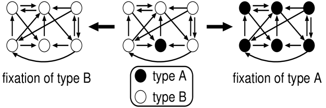
Figure 1: Fixation of type $A$ or type $B$ after introduction of a type $A$ mutant.

Consider the introduction of a single mutant of type $A$ at node $v_{i}$ in a population of $N-1$ residents of type $B$. Then, type $A$ either eventually fixates, i.e., takes over the entire population, or becomes extinct (i.e., fixation of $B$), as schematically shown in Fig. 1. We are concerned with the fixation probability of type $A$, which is denoted by $F_{i}$. When needed, we refer to any one of the three update rules introduced below by the superscript of $F_{i}$, such as $F_{i}^{LD}$ and $F_{i}^{IP}$. Throughout the paper, we assume that $G$ is strongly connected. A network is strongly connected if there is at least one directed path between any ordered pair of nodes. If $G$ is not strongly connected, we can find two nodes $v_{i}$ and $v_{j}$ such that there is no direct path from $v_{i}$ to $v_{j}$. In this case, the fixation probability $F_{i}$ is always zero because the individual at $v_{j}$ is never replaced by the mutant initially located at $v_{i}$ [3]. Therefore, it is sufficient to investigate fixation probabilities in the most upstream strongly connected component of $G$. Therefore, we assume without loss of generality that $G$ is strongly connected.

3 Results

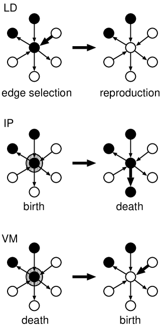
Figure 2: Schematics of three update rules.

In this section, we analytically obtain a system of linear equations that gives the fixation probabilities of mutants at individual nodes for the three update rules (link dynamics (LD), invasion process (IP), and voter model (VM)) [4, 5]. An update event in the three rules is schematically shown in Fig. 2. Then, we compare the analytical results with numerical results obtained for various directed networks.

3.1 Link dynamics (LD)

Firstly, we consider the LD [4, 5]. In this case, one directed edge is selected for reproduction in each time step; the edge $(v_{i},v_{j})\in E$ is chosen with probability $f_{i}w_{ij}/\sum_{k,l}f_{k}w_{kl}$ for the type of the individual at $v_{i}$ to replace the type of the individual at $v_{j}$. Individuals with larger fitness values and larger outgoing edge weights are more likely to reproduce than those with smaller fitness values and outgoing edge weights. Thus, the selection process acts on birth events. Alternatively, the selection process can be assumed to act on death events, and the edge $(v_{i},v_{j})$ is chosen with probability $(w_{ij}/f_{j})/(\sum_{k,l}w_{kl}/f_{l})$ for the type at $v_{i}$ to replace that at $v_{j}$. This implies that individuals with smaller fitness values and larger incoming edge weights are more likely to die than those with larger fitness values and smaller incoming edge weights. In fact, the fixation probability $F_{i}^{LD}$ ($1\leq i\leq N$) is the same under these two interpretations.

We consider the case $r=1$ (hence, $f_{i}=1$, $1\leq i\leq N$) analytically. Suppose that a single mutant of type $A$ invades $v_{i}$. The fixation probability is given by $F_{i}^{LD}$. By considering the next update event, we can recalculate $F_{i}^{LD}$ as follows. With probability $w_{ij}/\sum_{k,l}w_{kl}$, the edge $(v_{i},v_{j})\in E$ is selected for reproduction. Then, type $A$ individuals occupy $v_{i}$ and $v_{j}$. We denote by $F_{\{i,j\}}^{LD}$ the fixation probability when type $A$ individuals are initially located at $v_{i}$ and $v_{j}$ but nowhere else. With probability $w_{ji}/\sum_{k,l}w_{kl}$, the edge $(v_{j},v_{i})\in E$ is selected. Then, type $A$ becomes extinct, and type $A$ will not fixate. With the remaining probability $\sum_{k\neq i,l\neq i}w_{kl}/\sum_{k,l}w_{kl}$, the configuration of type $A$ and type $B$ individuals does not change. Therefore, we obtain

$$F_{i}^{LD}=\sum_{j}\frac{w_{ij}}{\sum_{k,l}w_{kl}}F_{\{i,j\}}^{LD}+\frac{\sum_{j}w_{ji}}{\sum_{k,l}w_{kl}}\times 0+\frac{\sum_{k\neq i,l\neq i}w_{kl}}{\sum_{k,l}w_{kl}}F_{i}^{LD}.$$ (1)

To prove $F_{\{i,j\}}^{LD}=F_{i}^{LD}+F_{j}^{LD}$, consider for now $N$ neutral types labeled 1, 2, $\ldots$, $N$ that are initially placed at $v_{1}$, $v_{2}$, $\ldots$ $v_{N}$, respectively. On a finite graph $G$, one of the $N$ types fixates eventually. The probability that type $i$ or $j$ fixates is given in two ways: $F_{\{i,j\}}^{LD}$ and $F_{i}^{LD}+F_{j}^{LD}$. This ends the proof. Using $F_{\{i,j\}}^{LD}=F_{i}^{LD}+F_{j}^{LD}$, we rearrange Eq.  (1) as

$$\sum_{j}w_{ij}F_{j}^{LD}=F_{i}^{LD}\sum_{j}w_{ji}.$$ (2)

This is a system of linear equations giving $F_{i}^{LD}$. We note that $F_{i}^{LD}$ can be interpreted as the reproductive value of the individual at node $v_{i}$ [20, 21].

Equation (2) can be derived more rigorously via the dual process [2, 22, 7, 1]. Intuitively speaking, the dual process of a stochastic process is another stochastic process in which the time of the original process is reversed. The direction of edges in the dual process is the opposite to that in the original process. By considering the dual process, we can understand the tree of family lines in the original process, which is called genealogy. When we go backward in time, two individuals sometimes ‘collide’ in the dual process. Such an event is called coalescence. In terms of the original process, a coalescence corresponds to two individuals sharing the common ancestor. After two individuals coalesce in the dual process, they behave as a single individual, representing a single family line. As far as the fixation probability is concerned, LD with $r=1$ is equivalent to the continuous-time stochastic process in which each edge $(v_{i},v_{j})\in E$ is selected for reproduction at the Poisson rate $w_{ij}$. Then, the dual process of LD is the continuous-time coalescing random walk on the network with all edges reversed, with a random walker initially located on every node [2, 1]. Coalescing random walk is defined as follows. Consider a walker at $v_{i}$ moving to $v_{j}$ at the Poisson rate $w_{ji}$. If there is another walker at $v_{j}$, the two walkers coalesce into one at $v_{j}$ and thereafter behave as a single random walker. On a finite graph $G$, the $N$ walkers eventually coalesce into one, which is consistent with the fact that the ancestors of all individuals are the same in the end. Then, $F_{i}^{LD}$ is the stationary density of the single random walker at $v_{i}$, which is given by Eq.  (2). As $G$ is strongly connected, the random walk on $G$ with all edges reversed defines an irreducible Markov chain. Because $F_{i}^{LD}$ is the stationary density of this irreducible Markov chain, Eq. (2) with constraints $\sum_{i=1}^{N}F_{i}^{LD}=1$ and $F_{i}^{LD}\geq 0$ always has a unique strictly positive solution.

The calculation of $F_{i}^{LD}$ from Eq. (2) by using a standard method such as the Gaussian elimination requires $O(N^{3})$ computation time. However, because relevant large networks are usually sparse, carrying out the Jacobi iteration may take much less time. The convergence of this iteration to ${\mathbf{F}}^{LD}$ is guaranteed by the Perron-Frobenius theorem [23].

In undirected graphs, $w_{ij}=w_{ji}$ holds. Therefore, $F_{i}^{LD}=1/N$ solves Eq. (2), giving a result previously reported in [4, 5]. In the case of weighted or directed networks, the complexity of Eq. (2) implies that $F_{i}^{LD}$ is not always determined by the local characteristics of node $v_{i}$ but is affected by the global structure of the networks.

Next, we argue that the mean-field (MF) approximation are not useful in most cases. Consider unweighted, but possibly directed, networks such that $w_{ij}=1$ if $(v_{i},v_{j})\in E$ and $w_{ij}=0$ otherwise. Let $k_{i}^{in}$ ($k_{i}^{out}$) be the indegree (outdegree) of $v_{i}$, and we set

$$\bar{F}^{LD}=\frac{1}{N}\sum^{N}_{i=1}F_{i}^{LD}.$$ (3)

The relation $\sum_{j}w_{ji}=k_{i}^{in}$, combined with the MF approximation $\sum_{i}w_{ij}F_{j}^{LD}\approx\sum_{i}w_{ij}\bar{F}^{LD}=k_{i}^{out}\bar{F}^{LD}$, yields

$$F_{i}^{LD}\propto\frac{k_{i}^{out}}{k_{i}^{in}}.$$ (4)

Equation (4) indicates that a large $k_{i}^{out}$ aids in the dissemination of the type at $v_{i}$ and a small $k_{i}^{in}$ inhibits the replacement of the type at $v_{i}$ by the type at other nodes.

However, the MF approximation deviates from the correct $F_{i}^{LD}$ in many cases. As an example, consider the largest strongly connected component of a directed and unweighted email social network [13] with $N=9079$ nodes and $\left<k\right>=\left<k^{in}\right>=\left<k^{out}\right>=2.62$, where $\langle\cdot\rangle$ denotes the average over the nodes. In this case, $F_{i}^{LD}$ (indicated by the circles in Fig. 3(c)) does not agree with the normalized $k_{i}^{out}/k_{i}^{in}$ (indicated by the line). This is mainly because the indegree and outdegree of the same node in this network are positively correlated and because this network presumably has a nontrivial global structure. Actually, the Pearson correlation coefficient (PCC) for the $N$ pairs ($k_{i}^{in}$, $k_{i}^{out}$), $1\leq i\leq N$, defined by

$$\frac{\frac{1}{N}\sum_{i=1}^{N}\left(k_{i}^{in}k_{i}^{out}-\left<k\right>^{2}\right)}{\sqrt{\frac{1}{N}\sum_{i=1}^{N}\left(k_{i}^{in}-\left<k\right>\right)^{2}}\sqrt{\frac{1}{N}\sum_{i=1}^{N}\left(k_{i}^{out}-\left<k\right>\right)^{2}}}$$ (5)

is equal to 0.40. Networks in which degrees of adjacent nodes are correlated also show considerable discrepancies between the MF approximation and the numerical results. On the other hand, in the case of undirected networks, our result $F_{i}^{LD}=1/N$ holds true in the presence of degree correlation of any kind, which is consistent with previously obtained numerical results [5].

Next, we examine the fixation probability in an asymmetric small-world network constructed from a ring of $N=5000$ nodes. This network is a directed version of the Watts-Strogatz small-world network [24]. Each node of this network tentatively sends directed edges to 5 nearest nodes along both sides. Then, 2500 out of $10N=50000$ directed edges are rewired so that their two ends are randomly and independently selected from the $N$ nodes, excluding self-loops and preexisting edges. The correlation between the in- and out-degrees of the same node is negligible, with the PCC for the pairs ($k_{i}^{in}$, $k_{i}^{out}$), defined by Eq. (5), being equal to $-0.021$. The degrees of adjacent nodes $v_{i}$ and $v_{j}$ conditioned by the existence of the edge ($v_{i}$, $v_{j}$) [25, 26] are also uncorrelated by the definition of the model. Nevertheless, the MF approximation is not effective in predicting the actual $F_{i}^{LD}$, as shown in Fig. 3(d). This discrepancy persists even for large $N$, because the directed small-world network does not render $F_{i}^{LD}$ of adjacent nodes independent of each other. In contrast, $F_{i}^{LD}$ in undirected small-world networks is completely determined by the MF ansatz indicated by the line in Fig. 3(d).

In contrast to these networks, Figure 3(a) shows that the MF relation $F_{i}^{LD}\propto k_{i}^{out}/k_{i}^{in}$ roughly holds for a directed random graph with $N=5000$. We generate a directed random graph by connecting each ordered pair of nodes $(v_{j},v_{j})$ with probability $2\left<k\right>/(N-1)$, so that $\left<k^{in}\right>=\left<k^{out}\right>=\left<k\right>$. In this network, degree correlation and macroscopic network structure are both absent, which enables the application of the MF approximation. Even in this network, however, the MF approximation is not exact because, as Eq. (2) predicts, $F_{i}^{LD}$ of nearby nodes are positively correlated. Following [26], we measure the correlation, or the assortativity, of $F_{i}^{LD}$ by the PCC for the pairs ($F_{i}^{LD}$, $F_{j}^{LD}$) for $(v_{i},v_{j})\in E$ defined by

$$\frac{\frac{1}{N}\sum_{(i,j)\in E}\left(F_{i}^{LD}F_{j}^{LD}-\left(\bar{F}^{LD}\right)^{2}\right)}{\frac{1}{N}\sum_{(i,j)\in E}^{N}\left(F_{i}^{LD}-\bar{F}^{LD}\right)^{2}},$$ (6)

where $\bar{F}^{LD}$ is defined by Eq. (3). The value of the PCC turns out to be slightly but significantly positive (mean $\pm$ standard deviation based on 100 network realizations is equal to 0.0834 $\pm$ 0.0057). The discrepancy is also significant for a large $N$, unless the mean degree $\left<k\right>$ is large.

The results obtained for random networks extend to the case of scale-free networks without degree correlation. We generate a directed scale-free network by setting the degree distribution to be $p(k)\propto k^{-3}$ for $k\geq\left<k\right>/2$ and $p(k)=0$ for $k<\left<k\right>/2$, thereby generating $k_{i}^{in}$ and $k_{i}^{out}$ ($1\leq i\leq N$) independently according to $p(k)$, and randomly connecting the nodes using the Molloy-Reed algorithm [27]. Figure 3(b) indicates that the MF approximation roughly explains the numerically obtained fixation probability.

It is noted that the PCC for the pairs ($F_{i}^{LD}$, $F_{j}^{LD}$) for $(v_{i},v_{j})\in E$ is small for the asymmetric scale-free network ($=0.0395\pm 0.0056$), is large for the asymmetric small-world network ($=0.7888\pm 0.0165$), and is small for the email social network ($=0.0420$).

3.2 Invasion process (IP)

Next, consider the IP [4, 5]. In the IP, selection acts on birth. In each time step, $v_{i}$ is first selected for reproduction with probability $f_{i}/\sum_{k}f_{k}$, where $f_{i}\in\{r,1\}$ is the fitness of the type at node $v_{i}$. Then, with probability $w_{ij}/\sum_{l}w_{il}$, the type at $v_{i}$ replaces that at $v_{j}$. Consequently, the probability that the edge $(v_{i},v_{j})\in E$ is used for reproduction in an update step is equal to $f_{i}w_{ij}/(\sum_{k}f_{k}\sum_{l}w_{il})$. On the complete graph, IP is the same as the standard Moran process [6]. For an arbitrary $r$ the IP is mapped to the LD with the rescaled edge weight $w_{ij}^{\prime}=w_{ij}/\sum_{l}w_{il}$. Therefore, from Eq. (2), the fixation probability for $r=1$ is the solution to

$$\sum_{j}\frac{w_{ij}}{\sum_{l}w_{il}}F_{j}^{IP}=F_{i}^{IP}\sum_{j}\frac{w_{ji}}{\sum_{l}w_{jl}}.$$ (7)

In the case of undirected unweighted networks, $F_{i}^{IP}\propto 1/k_{i}$ solves Eq. (7), giving a previously obtained result [4, 5, 22]. In the case of directed unweighted networks, applying the MF approximation to Eq. (7) yields

$$F_{i}^{IP}=\frac{\sum_{j,(i,j)\in E}F_{j}^{IP}/k_{i}^{out}}{\sum_{j,(j,i)\in E}1/k_{j}^{out}}\approx\frac{(const)}{k_{i}^{in}}.$$ (8)

The numerical results for the asymmetric random graph that is used for obtaining the results shown in Fig. 3(a) are shown in Fig. 4(a). The relation $F_{i}^{IP}\propto 1/k_{i}^{in}$ (the line in Fig. 4(a)) is roughly satisfied. Similar to the case of LD, some deviation persists in the case of random networks even with a large $N$. In contrast, Fig. 4(b) indicates that the actual $F_{i}^{IP}$ in the scale-free network deviates considerably from Eq. (8), mainly because of the discreteness of $k_{i}^{in}$ for a small integer $k_{i}^{in}$. Similar to the case of LD, the discrepancy between Eq. (8) and the exact $F_{i}^{IP}$ is also large in the case of the email social network (Fig. 4(c)) and the asymmetric small-world network (Fig. 4(d)). In addition to the degree correlation or global structure of networks, the discreteness of $1/k_{i}^{in}$ for a small $k_{i}^{in}$ causes further deviation, as shown in Figs. 4(c) and 4(d).

3.3 Voter model (VM)

We examine a third update rule, the so-called voter model (VM) [4, 5]. In the VM, we first eliminate the type at one node $v_{j}$ with probability $f_{j}^{-1}/\sum_{k}f_{k}^{-1}$. Then, with probability $w_{ij}/\sum_{l}w_{lj}$, the type at $v_{i}$ replaces that at $v_{j}$. The probability that the edge $(v_{i},v_{j})\in E$ is used for reproduction in an update step is equal to $f_{j}^{-1}w_{ij}/(\sum_{k}f_{k}^{-1}\sum_{l}w_{lj})$. For general $r$, the VM is mapped to the LD with the rescaled edge weight $w_{ij}^{\prime}=w_{ij}/\sum_{l}w_{lj}$. Consequently, from Eq. (2), $F_{i}^{VM}$ for $r=1$ is given by

$$\sum_{j}\frac{w_{ij}}{\sum_{l}w_{lj}}F_{j}^{VM}=F_{i}^{VM}\sum_{j}\frac{w_{ji}}{\sum_{l}w_{li}}\;\;(=F_{i}^{VM}).$$ (9)

In the case of undirected networks, $F_{i}^{VM}\propto k_{i}$ solves Eq. (9), recovering a previously obtained result [4, 5, 22]. The MF approximation yields

$$F_{i}^{VM}=\frac{\sum_{j,(i,j)\in E}F_{j}^{VM}}{k^{in}_{j}}\approx(const)\times k_{i}^{out}.$$ (10)

In the case of the random network and the uncorrelated scale-free network, the numerical results shown in Fig. 5(a) and Fig. 5(b), respectively, support the rough validity of Eq. (10). However, this naive ansatz deviates from the actual $F_{i}^{VM}$ for the email social network (Fig. 5(c)) and the asymmetric small-world network (Fig. 5(d)). This situation is similar to that observed in the case of LD.

The fixation probability $F_{i}^{VM}$ on a graph $G$ is equivalent to the PageRank of node $v_{i}$ of the graph $G^{\prime}$, where $G^{\prime}$ is constructed by reversing all edges of $G$. The PageRank measures the number of directed edges a node, such as a webpage, receives from other important nodes as exclusively as possible [28, 29, 30]. If we neglect some minor technical treatments that are necessary for the practical implementation, the PageRank $F_{i}^{PR}$ of $v_{i}$ is defined by

$$\sum_{j}\frac{w_{ji}}{\sum_{l}w_{jl}}F_{j}^{PR}=\lambda F_{i}^{PR},$$ (11)

where $\lambda$ is the largest eigenvalue of the eigenequation (11). If many edges are directed to $v_{i}$, there are many positive terms (i.e., $w_{ji}>0$) on the LHS of Eq. (11), and they contribute to the PageRank of $v_{i}$ on the RHS. If $v_{i}$ receives an edge from $v_{j}$ whose outdegree is small or whose PageRank is large, $w_{ji}/\sum_{l}w_{jl}$ or $F_{j}^{PR}$ is large. Each of these factors also increases $F_{i}^{PR}$. A strongly connected network yields $\lambda=1$, so that $F_{i}^{PR}$ is the stationary density of the discrete-time simple random walk on the original graph $G$ [23, 28, 29, 30]. Equation (11) with $\lambda=1$ and with $w_{ij}$ replaced by $w_{ji}$ is identical to Eq. (9). In PageRank, nodes that receive many edges tend to be important, whereas the opposite is true in the case of the VM. $F_{i}^{PR}$ is locally approximated by using $k_{i}^{in}$ [31], which corresponds to the MF relation $F_{i}^{VM}\propto k_{i}^{out}$. However, $F_{i}^{PR}$ in real web graphs often deviates from the relation $F_{i}^{PR}\propto k_{i}^{in}$ [32]. This implies that $F_{i}^{VM}$ in real networks can also deviate from the MF approximation, which is consistent with our main claim.

3.4 Constant selection ($r\neq 1$)

When $r\neq 1$, the fitness value of type A and that of type B are different, so one type has a unilateral advantage over the other type. We call this situation ‘constant selection’. In this case, the dual process of the evolutionary dynamics is the coalescing and branching random walk [2], which is difficult to handle analytically. Therefore, we carry out Monte Carlo simulations for $r=4$ on a fixed asymmetric random graph with $N=200$ and $\left<k\right>=10$. We calculate $F_{i}^{LD}$ as a fraction of runs from $2\times 10^{6}$ runs in which the single mutant with fitness $r$ initially located at $v_{i}$ (i.e., $f_{i}=r$ and $f_{j}=1$, $j\neq i$) eventually occupies all nodes of the network. In Fig. 6(a), the numerically obtained $F_{i}^{LD}$ for $r=4$ is plotted against the exact solution of $F_{i}^{LD}$ for $r=1$ (Eq.  (2)). Roughly speaking, $F_{i}^{LD}$ for $r=4$ monotonically increases with the exactly obtained $F_{i}^{LD}$ for $r=1$. We obtain similar results in the case of the IP (Fig. 6(b)) and VM (Fig. 6(c)). Therefore, the node from which a mutant is more likely to propagate throughout the population under the neutral dynamics ($r=1$) also serves as a better invading node for mutants under the constant selection ($r\in 1$). Thus, our results derived in the case of the neutral selection is useful in predicting the order of the maginitude of fixation probabilities under the constant selection.

3.5 Modular networks

Real networks are often more complex than degree-uncorrelated random, scale-free, or small-world networks. In particular, many networks are modular, i.e., they consist of several densely connected subgraphs termed modules, and each subgraph is connected to each other by a relatively few edges [33]. This is also the case for directed [34, 35] and weighted [36] networks.

To intuitively understand the importance of the global structure of networks such as community structure in evolutionary dynamics, we generate a modular network [35], as schematically shown in Fig. 7(a), and study the fixation probability under neutrality, i.e., $r=1$. We generate two modules $M_{1}=\{v_{1},\ldots,v_{N/2}\}$ and $M_{2}=\{v_{N/2+1},\ldots,v_{N}\}$ as two directed random graphs with $N/2=2500$ nodes and the mean degree $\left<k\right>_{M}=10$. Then, we randomly connect $M_{1}$ and $M_{2}$ by directed edges so that a node in $M_{1}$ ($M_{2}$) has $w_{1\to 2}\left<k\right>_{M}$ ($w_{2\to 1}\left<k\right>_{M}$) outgoing edges to the nodes in $M_{2}$ ($M_{1}$) on an average. By setting $w_{1\to 2}=0.04$ and $w_{2\to 1}=0.01$, we obtain a network with $N=5000$ and $\left<k\right>=10.25$. Note that the degree correlation is absent in this network. For the realized network, $F_{i}^{LD}$ for $r=1$ is shown in Fig. 7(b). Rather than the MF ansatz $\propto k_{i}^{out}/k_{i}^{in}$ (solid line), the module membership is the main determinant of $F_{i}^{LD}$. The upper and lower sets of points in Fig. 7(b) correspond to the nodes in $M_{1}$ and $M_{2}$, respectively. The magnitude of $F_{i}^{LD}$ in the two sets differ approximately by a factor of $w_{1\to 2}/w_{2\to 1}=4$. The results obtained in the case of the IP and VM are similar, as shown in Figs. 7(c) and 7(d), respectively. There, gross connectivity among modules, not local degrees, principally determines $F_{i}$. An modified ansatz that combines the MF approximation and the multiplicative factor determined by the module membership of the node

$$F_{i}^{LD}\propto\left\{\begin{array}[]{ll}w_{1\to 2}k_{i}^{out}/k_{i}^{in},&v_{i}\in M_{1}\\ w_{2\to 1}k_{i}^{out}/k_{i}^{in},&v_{i}\in M_{2}\end{array}\right.$$ (12)

fits the data well (the dashed lines in Fig. 7(b)). Similar approximations in which $k_{i}^{out}/k_{i}^{in}$ in Eq. (12) is replaced with $1/k_{i}^{in}$ and $k_{i}^{out}$ (dashed lines in Figs. 7(b) and 7(c), respectively) roughly agree with the observed $F_{i}^{IP}$ and $F_{i}^{VM}$.

To explain this result analytically, we presume that all nodes in a module are equivalent and have an identical fixation probability, $\hat{F}_{1}$ or $\hat{F}_{2}$. In this manner, a network with two modules is reduced to a network with two nodes and self-loops. Equation (2) with $N=2$ yields

$$\hat{F}_{1}^{LD} = \frac{w_{12}}{w_{12}+w_{21}},$$ (13)

$$\hat{F}_{2}^{LD} = \frac{w_{21}}{w_{12}+w_{21}}.$$ (14)

Because $w_{11}=w_{22}=\left<k\right>_{M}$, $w_{12}=w_{1\to 2}\left<k\right>_{M}$, and $w_{21}=w_{2\to 1}\left<k\right>_{M}$, we obtain

$$\frac{\hat{F}_{1}^{LD}}{\hat{F}_{2}^{LD}}=\frac{w_{1\to 2}}{w_{2\to 1}},$$ (15)

which agrees with the numerical results. On the other hand, $k_{i}^{out}/k_{i}^{in}$ is equal to $(1+w_{1\to 2})/(1+w_{2\to 1})$ and $(1+w_{2\to 1})/(1+w_{1\to 2})$ for $M_{1}$ and $M_{2}$, respectively. Both of these values are close to unity when $w_{1\to 2},w_{2\to 1}\ll 1$, i.e., when the network is modular. Therefore, the MF approximation gives $\hat{F}_{1}^{LD}/\hat{F}_{2}^{LD}\approx 1$, which is different from our simulated results.

Similar calculations in the case of the IP yield

$$\hat{F}_{i}^{IP}=\frac{C^{IP}_{i}}{C^{IP}_{1}+C^{IP}_{2}},\quad(i=1,2)$$ (16)

where

$$C^{IP}_{1} \equiv \frac{w_{12}}{w_{11}+w_{12}},$$ (17)

$$C^{IP}_{2} \equiv \frac{w_{21}}{w_{21}+w_{22}}.$$ (18)

Therefore, we obtain

$$\frac{\hat{F}_{1}^{IP}}{\hat{F}_{2}^{IP}}\approx\frac{w_{1\to 2}}{w_{2\to 1}}$$ (19)

when $w_{1\to 2},w_{2\to 1}\ll 1$. However, the naive MF ansatz (Eq. (8)) yields $1/k_{i}^{in}=1/\left(\left<k\right>(1+w_{2\to 1})\right)\approx 1/\left<k\right>$ ($1\leq i\leq N/2$) and $1/k_{i}^{in}=1/\left(\left<k\right>(1+w_{1\to 2})\right)\approx 1/\left<k\right>$ ($(N/2)+1\leq i\leq N$). Then, $\hat{F}_{1}^{IP}/\hat{F}_{2}^{IP}$ would be approximately unity, which does not well explain the simulation results shown in Fig. 7(c).

In the case of the VM, we obtain

$$\hat{F}_{i}^{VM}=\frac{C^{VM}_{i}}{C^{VM}_{1}+C^{VM}_{2}},$$ (20)

where

$$C^{VM}_{1} \equiv \frac{w_{12}}{w_{12}+w_{22}},$$ (21)

$$C^{VM}_{2} \equiv \frac{w_{21}}{w_{11}+w_{21}}.$$ (22)

When $w_{1\to 2},w_{2\to 1}\ll 1$, we obtain

$$\frac{\hat{F}_{1}^{VM}}{\hat{F}_{2}^{VM}}\approx\frac{w_{1\to 2}}{w_{2\to 1}}.$$ (23)

However, the naive MF ansatz (Eq. (10)) yields $k_{i}^{out}=\left<k\right>(1+w_{1\to 2})\approx\left<k\right>$ ($1\leq i\leq N/2$) and $k_{i}^{out}=\left<k\right>(1+w_{1\to 2})\approx\left<k\right>$ ($N/2+1\leq i\leq N$). Then, $\hat{F}_{1}^{VM}/\hat{F}_{2}^{VM}$ would be approximately unity, which again does not explain the simulation results shown in Fig. 7(d).

In sum, for each update rule the community structure of networks has a strong impact on the fixation probability.

4 Conclusions

In summary, we obtained general formulae for the fixation probability in directed and weighted networks. For each of the three different update rules, fixation probability is a solution to a system of linear equations. Fixation probability in undirected networks is completely determined by the local connectivity [4, 5] under neutrality. In contrast, in the case of directed degree-correlated, small-world, or modular networks, fixation probability is not determined only by the degree of the node that a mutant initially invades, and it deviates from the MF approximation to a large extent. Our results indicate that the global connectivity of networks has a significant effect on the fixation probability.

Figure 3: $F_{i}^{LD}$ (i.e., the fixation probability under LD) for a single mutant initially at node $v_{i}$ in (a) an asymmetric random network with $N=5000$, (b) an asymmetric scale-free network with $N=5000$, (c) largest strongly connected component of email social network with $N=9079$, and (d) an asymmetric small-world network with $N=5000$. The normalized $k_{i}^{out}/k_{i}^{in}$ is equal to $(k_{i}^{out}/k_{i}^{in})/\sum_{j=1}^{N}(k_{j}^{out}/k_{j}^{in})$. The lines represent the MF ansatz $F_{i}^{LD}=(k_{i}^{out}/k_{i}^{in})/\sum_{j=1}^{N}(k_{j}^{out}/k_{j}^{in})$.

Figure 4: $F_{i}^{IP}$ in (a) asymmetric random network, (b) asymmetric scale-free network, (c) email social network, and (d) asymmetric small-world network. The normalized $1/k_{i}^{in}$ is equal to $(1/k_{i}^{in})/\sum_{j=1}^{N}(1/k_{j}^{in})$. The lines represent the MF ansatz $F_{i}^{IP}=(1/k_{i}^{in})/\sum_{j=1}^{N}(1/k_{j}^{in})$.

Figure 5: $F_{i}^{VM}$ in (a) asymmetric random network, (b) asymmetric scale-free network, (c) email social network, and (d) asymmetric small-world network. The normalized $k_{i}^{out}$ is equal to $k_{i}^{out}/\sum_{j=1}^{N}k_{j}^{out}$. The lines represent the MF ansatz $F_{i}^{VM}=k_{i}^{out}/\sum_{j=1}^{N}k_{j}^{out}$.

Figure 6: (a) $F_{i}^{LD}$ for $r=4$ plotted against $F_{i}^{LD}$ for $r=1$. (b) $F_{i}^{IP}$ for $r=4$ plotted against $F_{i}^{IP}$ for $r=1$. (c) $F_{i}^{VM}$ for $r=4$ plotted against $F_{i}^{VM}$ for $r=1$. We have used an asymmetric random network with $N=200$.

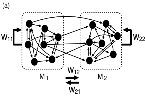
Figure 7: (a) Example of modular network, with $w_{11}$, $w_{12}$, $w_{21}$, and $w_{22}$ indicating edge weights when this network is coarse grained as two-node network. (b) $F_{i}^{LD}$, (c) $F_{i}^{IP}$, and (d) $F_{i}^{VM}$ in an asymmetric modular network with $N=5000$. The solid lines represent the meanfield ansatz (see the captions of Figs. 3, 4, and 5 for details). The dashed lines represent the ansatz derived from the combination of the local degree and the module membership of the node (see Eq. (12) for the expression in case of LD).

References

- [1] Liggett T M 1985 Interacting Particle Systems (New York: Springer)
- [2] Durrett D 1988 Lecture Notes on Particle Systems and Percolation (Belmont, CA: Wadsworth)
- [3] Lieberman E, Hauert C and Nowak M A 2005 Nature 433 312
- [4] Antal T, Redner S and Sood V 2006 Phys. Rev. Lett. 96 188104
- [5] Sood V, Antal T and Redner S 2008 Phys. Rev. E 77 041121
- [6] Moran P A P 1958 Proc. Camb. Phil. Soc. 54 60
- [7] Ewens W J 2004 Mathematical Population Genetics (New York: Springer)
- [8] Nowak M A 2006 Evolutionary Dynamics — Exploring the Equations of Life (Cambridge: The Belknap Press of Harvard University Press)
- [9] Castellano C, Vilone D and Vespignani A 2003 Europhys. Lett. 63 153
- [10] Sood V and Redner S 2005 Phys. Rev. Lett. 94 178701
- [11] Suchecki K, Eguíluz V M and San Miguel M 2005 Phys. Rev. E 72 036132
- [12] Vazquez F and Eguíluz V M 2008 New J. Phys. 10 063011
- [13] Ebel H, Mielsch L-I and Bornholdt S 2002 Phys. Rev. E 66 035103(R)
- [14] Sade D S 1972 Folia Primat. 8 196
- [15] Newman M E J, Forrest S and Balthrop J 2002 Phys. Rev. E 66 035101(R)
- [16] Gustafson E J and Gardner R H 1996 Ecology 77 94
- [17] Schooley R L and Wiens J A 2003 Oikos 102 559.
- [18] Schick R S and Lindley S T 2007 J. Appl. Ecol. 44 1116
- [19] Barrat A, Barthélemy M, Pastor-Satorras R and Vespignani A 2004 Proc. Natl. Acad. Sci. USA 101 3747
- [20] Taylor P D 1990 Amer. Natur. 135 95
- [21] Taylor P D 1996 J. Math. Biol. 34 654
- [22] Donnelly P and Welsh D 1983 Math. Proc. Camb. Phil. Soc. 94 167
- [23] Horn R A and Johnson C R 1985 Matrix Analysis (Cambridge: Cambridge University Press)
- [24] Watts D J and Strogatz S H 1998 Nature 393 440
- [25] Newman M E J 2002 Phys. Rev. Lett. 89 208701
- [26] Newman M E J 2003 Phys. Rev. E 67 026126
- [27] Molloy M and Reed B 1998 Comb. Prob. Comput. 7 295
- [28] Brin S and Page L 1998 Proc. 7th Int. World Wide Web Conf. (Brisbane, Australia, 14–18 April) p 107
- [29] Berkhin P 2005 Internet Math. 2 73
- [30] Langville A N and Meyer C D 2005 SIAM Rev. 47 135
- [31] Fortunato S, Boguñá M, Flammini A and Menczer F 2006 Proc. 4th Workshop on Algorithms and Models for the Web Graph (WAW 2006), (Edinburgh, UK, 22–26 May) p 59
- [32] Donato D, Laura L, Leonardi S and Millozzi S 2004 Eur. Phys. J. B 38 239
- [33] Girvan M and Newman M E J 2002 Proc. Natl. Acad. Sci. USA 99 7821
- [34] Palla G, Farkas I J, Pollner P, Derényi I and Vicsek T 2007 New J. Phys. 9 186
- [35] Leicht E A and Newman M E J 2008 Phys. Rev. Lett. 100 118703
- [36] Farkas I J, Ábel D, Palla G and Vicsek T 2007 New J. Phys. 9 180