Instabilities in the Æther
Abstract
We investigate the stability of theories in which Lorentz invariance is spontaneously broken by fixed-norm vector “æther” fields. Models with generic kinetic terms are plagued either by ghosts or by tachyons, and are therefore physically unacceptable. There are precisely three kinetic terms that are not manifestly unstable: a sigma model , the Maxwell Lagrangian , and a scalar Lagrangian . The timelike sigma-model case is well-defined and stable when the vector norm is fixed by a constraint; however, when it is determined by minimizing a potential there is necessarily a tachyonic ghost, and therefore an instability. In the Maxwell and scalar cases, the Hamiltonian is unbounded below, but at the level of perturbation theory there are fewer degrees of freedom and the models are stable. However, in these two theories there are obstacles to smooth evolution for certain choices of initial data.
I Introduction
The idea of spontaneous violation of Lorentz invariance through tensor fields with non-vanishing expectation values has garnered substantial attention in recent years Will and Nordtvedt (1972); Gasperini (1987); Kostelecky and Samuel (1989); Colladay and Kostelecky (1998); Jacobson and Mattingly (2001); Eling and Jacobson (2004); Carroll and Lim (2004); Jacobson and Mattingly (2004); Lim (2005); Eling et al. (2004); Dulaney et al. (2008); Jimenez and Maroto (2008). Hypothetical interactions between Standard Model fields and Lorentz-violating (LV) tensor fields are tightly constrained by a wide variety of experimental probes, in some cases leading to limits at or above the Planck scale Colladay and Kostelecky (1998); Kostelecky and Lehnert (2001); Carroll and Lim (2004); Elliott et al. (2005); Mattingly (2005); Will (2005); Jacobson (2008).
If these constraints are to be taken seriously, it is necessary to have a sensible theory of the dynamics of the LV tensor fields themselves, at least at the level of low-energy effective field theory. The most straightforward way to construct such a theory is to follow the successful paradigm of scalar field theories with spontaneous symmetry breaking, by introducing a tensor potential that is minimized at some non-zero expectation value, in addition to a kinetic term for the fields. (Alternatively, it can be a derivative of the field that obtains an expectation value, as in ghost condensation models Arkani-Hamed et al. (2004, 2007); Cheng et al. (2006).) As an additional simplification, we may consider models in which the nonzero expectation value is enforced by a Lagrange multiplier constraint, rather than by dynamically minimizing a potential; this removes the “longitudinal” mode of the tensor from consideration, and may be thought of as a limit of the potential as the mass near the minimum is taken to infinity. In that case, there will be a vacuum manifold of zero-energy tensor configurations, specified by the constraint.
All such models must confront the tricky question of stability. Ultimately, stability problems stem from the basic fact that the metric has an indefinite signature in a Lorentzian spacetime. Unlike in the case of scalar fields, for tensors it is necessary to use the spacetime metric to define both the kinetic and potential terms for the fields. A generic choice of potential would have field directions in which the energy is unbounded from below, leading to tachyons, while a generic choice of kinetic term would have modes with negative kinetic energies, leading to ghosts. Both phenomena represent instabilities; if the theory has tachyons, small perturbations grow exponentially in time at the linearized level, while if the theory has ghosts, nonlinear interactions create an unlimited number of positive- and negative-energy excitations Carroll et al. (2003). There is no simple argument that these unwanted features are necessarily present in any model of LV tensor fields, but the question clearly warrants careful study.
In this paper we revisit the question of the stability of theories of dynamical Lorentz violation, and argue that most such theories are unstable. In particular, we examine in detail the case of a vector field with a nonvanishing expectation value, known as the “æther” model or a “bumblebee” model. For generic choices of kinetic term, it is straightforward to show that the Hamiltonian of such a model is unbounded from below, and there exist solutions with bounded initial data that grow exponentially in time.
There are three specific choices of kinetic term for which the analysis is more subtle. These are the sigma-model kinetic term,
| (1) |
which amounts to a set of four scalar fields defined on a target space with a Minkowski metric; the Maxwell kinetic term,
| (2) |
where is familiar from electromagnetism; and what we call the “scalar” kinetic term,
| (3) |
featuring a single scalar degree of freedom. Our findings may be summarized as follows:
-
•
The sigma-model Lagrangian with the vector field constrained by a Lagrange multiplier to take on a timelike expectation value is the only æther theory for which the Hamiltonian is bounded from below in every frame, ensuring stability. In a companion paper, we examine the cosmological behavior and observational constraints on this model Carroll et al. (2009). If the vector field is spacelike, the Hamiltonian is unbounded and the model is unstable. However, if the constraint in the sigma-model theory is replaced by a smooth potential, allowing the length-changing mode to become a propagating degree of freedom, that mode is necessarily ghostlike (negative kinetic energy) and tachyonic (correct sign mass term), and the Hamiltonian is unbounded below, even in the timelike case. It is therefore unclear whether models of this form can arise in any full theory.
-
•
In the Maxwell case, the Hamiltonian is unbounded below; however, a perturbative analysis does not reveal any explicit instabilities in the form of tachyons or ghosts. The timelike mode of the vector acts as a Lagrange multiplier, and there are fewer propagating degrees of freedom at the linear level (a “spin-1” mode propagates, but not a “spin-0” mode). Nevertheless, singularities can arise in evolution from generic initial data: for a spacelike vector, for example, the field evolves to a configuration in which the fixed-norm constraint cannot be satisfied (or perhaps just to a point where the effective field theory breaks down). In the timelike case, a certain subset of initial data is well-behaved, but, provided the vector field couples only to conserved currents, the theory reduces precisely to conventional electromagnetism, with no observable violations of Lorentz invariance. It is unclear whether there exists a subset of initial data that leads to observable violations of Lorentz invariance while avoiding problems in smooth time evolution.
-
•
The scalar case is superficially similar to the Maxwell case, in that the Hamiltonian is unbounded below, but a perturbative analysis does not reveal any instabilities. Again, there are fewer degrees of freedom at the linear level; in this case, the spin-1 mode does not propagate. There is a scalar degree of freedom, but it does not correspond to a propagating mode at the level of perturbation theory (the dispersion relation is conventional, but the energy vanishes to quadratic order in the perturbations). For the timelike æther field, obstacles arise in the time evolution that are similar to those of a spacelike vector in the Maxwell case; for a spacelike æther field with a scalar action, the behavior is less clear.
-
•
For any other choice of kinetic term, æther theories are always unstable.
Interestingly, these three choices of æther dynamics are precisely those for which there is a unique propagation speed for all dynamical modes; this is the same condition required to ensure that the Generalized Second Law is respected by a Lorentz-violating theory Dubovsky and Sibiryakov (2006); Eling et al. (2007).
One reason why our findings concerning stability seem more restrictive than those of some previous analyses is that we insist on perturbative stability in all Lorentz frames, which is necessary in theories where the form of the Hamiltonian is frame-dependent. In a Lorentz-invariant field theory, it suffices to pick a Lorentz frame and examine the behavior of small fluctuations; if they grow exponentially, the model is unstable, while if they oscillate, the model is stable. In Lorentz-violating theories, in contrast, such an analysis might miss an instability in one frame that is manifest at the linear level in some other frame Kostelecky (2001); Mattingly (2005); Adams et al. (2006). This can be traced to the fact that a perturbation that is “small” in one frame (the value of the perturbation is bounded everywhere along some initial spacelike slice), but grows exponentially with time as measured in that frame, will appear “large” (unbounded on every spacelike slice) in some other frame.
As an explicit example, consider a model of a timelike vector with a background configuration , and perturbations , where is some constant polarization vector. In this frame, we will see that the dispersion relation takes the form
| (4) |
Clearly, the frequency will be real for every real wave vector , and such modes simply oscillate rather than growing in time. It is tempting to conclude that models of this form are perturbatively stable for any value of . However, we will see below that when , there exist other frames (boosted with respect to the original) in which can be real but is necessarily complex, indicating an instability. These correspond to wave vectors for which, evaluated in the original frame, both and are complex. Modes with complex spatial wave vectors are not considered to be “perturbations,” since the fields blow up at spatial infinity. However, in the presence of Lorentz violation, a complex spatial wave vector in one frame may correspond to a real spatial wave vector in a boosted frame. We will show that instabilities can arise from initial data defined on a constant-time hypersurface (in a boosted frame) constructed solely from modes with real spatial wave vectors. Such modes are bounded at spatial infinity (in that frame), and could be superimposed to form wave packets with compact support. Since the notion of stability is not frame dependent, the existence of at least one such frame indicates that the theory is unstable, even if there is no linear instability in the æther rest frame.
Several prior investigations have considered the question of stability in theories with LV vector fields. Lim Lim (2005) calculated the Hamiltonian for small perturbations around a constant timelike vector field in the rest frame, and derived restrictions on the coefficients of the kinetic terms. Bluhm et al. Bluhm et al. (2008a) also examined the timelike case with a Lagrange multiplier constraint, and showed that the Maxwell kinetic term led to stable dynamics on a certain branch of the solution space if the vector was coupled to a conserved current. It was also found, in Bluhm et al. (2008a), that most LV vector field theories have Hamiltonians that are unbounded below. Boundedness of the Hamiltonian was also considered in Chkareuli et al. (2006). In the context of effective field theory, Gripaios Gripaios (2004) analyzed small fluctuations of LV vector fields about a flat background. Dulaney, Gresham and Wise Dulaney et al. (2008) showed that only the Maxwell choice was stable to small perturbations in the spacelike case assuming the energy of the linearized modes was non-zero.111This effectively eliminates the scalar case. Elliot, Moore, and Stoica Elliott et al. (2005) showed that the sigma-model kinetic term is stable in the presence of a constraint, but not with a potential.
In the next section, we define notation and fully specify the models we are considering. We then turn to an analysis of the Hamiltonians for such models, and show that they are always unbounded below unless the kinetic term takes on the sigma-model form and the vector field is timelike. This result does not by itself indicate an instability, as there may not be any dynamical degree of freedom that actually evolves along the unstable direction. Therefore, in the following section we look carefully at linear stability around constant configurations, and isolate modes that grow exponentially with time. In the section after that we show that the models that are not already unstable at the linear level end up having ghosts, with the exception of the Maxwell and scalar cases. We then examine some features of those two theories in particular.
II Models
We will consider a dynamical vector field propagating in Minkowski spacetime with signature . The action takes the form
| (5) |
where is the kinetic Lagrange density and is (minus) the potential. A general kinetic term that is quadratic in derivatives of the field can be written222In terms of the coefficients, , defined in Jacobson and Mattingly (2004) and used in many other publications on æther theories, (6) where is the gravitational constant.
| (7) |
In flat spacetime, setting the fields to constant values at infinity, we can integrate by parts to write an equivalent Lagrange density as
| (8) |
where and we have defined
| (9) |
In terms of these variables, the models specified above with no linear instabilities or negative-energy ghosts are:
-
•
Sigma model: ,
-
•
Maxwell: , and
-
•
Scalar: ,
in all cases with .
The vector field will obtain a nonvanishing vacuum expectation value from the potential. For most of the paper we will take the potential to be a Lagrange multipler constraint that strictly fixes the norm of the vector:
| (10) |
where is a Lagrange multiplier whose variation enforces the constraint
| (11) |
If the upper sign is chosen, the vector will be timelike, and it will be spacelike for the lower sign. Later we will examine how things change when the constraint is replaced by a smooth potential of the form . It will turn out that the theory defined with a smooth potential is only stable in the limit as . In any case, unless we specify otherwise, we assume that the norm of the vector is determined by the constraint (11).
We are left with an action
| (12) |
The Euler-Lagrange equation obtained by varying with respect to is
| (13) |
where we have defined
| (14) |
Since the fixed-norm condition (11) is a constraint, we can consistently plug it back into the equations of motion. Multiplying (13) by and using the constraint, we can solve for the Lagrange multiplier,
| (15) |
Inserting this back into (13), we can write the equation of motion as a system of three independent equations:
| (16) |
The tensor acts to take what would be the equation of motion in the absence of the constraint, and project it into the hyperplane orthogonal to . There are only three independent equations because vanishes identically, given the fixed norm constraint.
II.1 Validity of effective field theory
As in this paper we will restrict our attention to classical field theory, it is important to check that any purported instabilities are found in a regime where a low-energy effective field theory should be valid. The low-energy degrees of freedom in our models are Goldstone bosons resulting from the breaking of Lorentz invariance. The effective Lagrangian will consist of an infinite series of terms of progressively higher order in derivatives of the fields, suppressed by appropriate powers of some ultraviolet mass scale . If we were dealing with the theory of a scalar field , the low-energy effective theory would be valid when the canonical kinetic term was large compared to a higher-derivative term such as
| (17) |
For fluctuations with wavevector , we have , and the lowest-order terms accurately describe the dynamics whenever . A fluctuation that has a low momentum in one frame can, of course, have a high momentum in some other frame, but the converse is also true; the set of perturbations that can be safely considered “low-energy” looks the same in any frame.
With a Lorentz-violating vector field, the situation is altered. In addition to higher-derivative terms of the form , the possibility of extra factors of the vector expectation value leads us to consider terms such as
| (18) |
The number of such higher dimension operators in the effective field theory is greatly reduced because and, therefore, . It can be shown that an independent operator with derivatives includes at most vector fields, so that the term highlighted here has the largest number of ’s with four derivatives. We expect that the ultraviolet cutoff is of order the vector norm, . Hence, when we consider a background timelike vector field in its rest frame,
| (19) |
the term reduces to , and the effective field theory is valid for modes with , just as in the scalar case.
But now consider a highly boosted frame, with
| (20) |
At large , individual components of will scale as , and the higher-derivative term schematically becomes
| (21) |
For modes with spatial wave vector (as measured in this boosted frame), we are therefore comparing with the canonical term . The lowest-order terms therefore only dominate for wave vectors with
| (22) |
In the presence of Lorentz violation, therefore, the realm of validity of the effective field theory may be considerably diminished in highly boosted frames. We will be careful in what follows to restrict our conclusions to those that can be reached by only considering perturbations that are accurately described by the two-derivative terms. The instabilities we uncover are infrared phenomena, which cannot be cured by changing the behavior of the theory in the ultraviolet. We have been careful to include all of the lowest order terms in the effective field theory expansion—the terms in (8).
III Boundedness of the Hamiltonian
We would like to establish whether there are any values of the parameters , and for which the æther model described above is physically reasonable. In practice, we take this to mean that there exist background configurations that are stable under small perturbations. It seems hard to justify taking an unstable background as a starting point for phenomenological investigations of experimental constraints, as we would expect the field to evolve on microscopic timescales away from its starting point.
“Stability” of a background solution to a set of classical equations of motion means that, for any small neighborhood of in the phase space, there is another neighborhood of such that the time evolution of any point in remains in for all times. More informally, small perturbations oscillate around the original background, rather than growing with time. A standard way of demonstrating stability is to show that the Hamiltonian is a local minimum at the background under consideration. Since the Hamiltonian is conserved under time evolution, the allowed evolution of a small perturbation will be bounded to a small neighborhood of that minimum, ensuring stability. Note that the converse does not necessarily hold; the presence of other conserved quantities can be enough to ensure stability even if the Hamiltonian is not bounded from below.
One might worry about invoking the Hamiltonian in a theory where Lorentz invariance has been spontaneously violated. Indeed, as we shall see, the form of the Hamiltonian for small perturbations will depend on the Lorentz frame in which they are expressed. To search for possible linear instabilities, it is necessary to consider the behavior of small perturbations in every Lorentz frame.
The Hamiltonian density, derived from the action (12) via a Legendre transformation, is
| (23) | ||||
| (24) |
where Latin indices run over . The total Hamiltonian corresponding to this density is
| (25) |
We have integrated by parts and assumed that vanishes at spatial infinity; repeated lowered indices are summed (without any factors of the metric). Note that this Hamiltonian is identical to that of a theory with a smooth (positive semi-definite) potential instead of a Lagrange multiplier term, evaluated at field configurations for which the potential is minimized. Therefore, if the Hamiltonian is unbounded when the fixed-norm constraint is enforced by a Lagrange multiplier, it will also be unbounded in the case of a smooth potential.
There are only three dynamical degrees of freedom, so we may reparameterize such that the fixed-norm constraint is automatically enforced and the allowed three-dimensional subspace is manifest. We define a boost variable and angular variables and , so that we can write
| (26) | ||||
| (27) |
in the timelike case with , and
| (28) | ||||
| (29) |
in the spacelike case with . In these expressions,
| (30) | ||||
| (31) | ||||
| (32) |
so that . In terms of this parameterization, the Hamiltonian density for a timelike æther field becomes
| (33) |
while for the spacelike case we have
| (34) |
Expressed in terms of the variables , the Hamiltonian is a function of initial data that automatically respects the fixed-norm constraint. We assume that the derivatives vanish at spatial infinity.
III.1 Timelike vector field
We can now determine which values of the parameters lead to Hamiltonians that are bounded below, starting with the case of a timelike æther field. We can examine the various possible cases in turn.
-
•
Case One: and .
-
•
Case Two: and .
In this case, consider configurations with , , , . Then we have
(36) For , the Hamiltonian can be arbitrarily negative for any value of .
-
•
Case Three: , , and .
We consider configurations with , , , , which gives
(37) Again, this can be arbitrarily negative.
-
•
Case Four: , , and .
Now we consider configurations with , , , . Then,
(38) which can be arbitrarily negative.
-
•
Case Five: .
Now we consider configurations with , and . Then,
(39) which can be arbitrarily negative for any non-zero and for any values of and .
For any case other than the sigma-model choice , it is therefore straightforward to find configurations with arbitrarily negative values of the Hamiltonian.
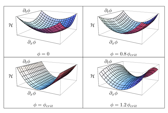
Nevertheless, a perturbative analysis of the Hamiltonian would not necessarily discover that it was unbounded. The reason for this is shown in Fig. 1, which shows the Hamiltonian density for the theory with , , in a restricted subspace where and , leaving only , , and as independent variables. We have plotted as a function of and for four different values of . When is sufficiently small, so that the vector is close to being purely timelike, the point is a local minimum. Consequently, perturbations about constant configurations with small would appear stable. But for large values of , the unboundedness of the Hamiltonian becomes apparent. This phenomenon will arise again when we consider the evolution of small perturbations in the next section. At the end of this section, we will explain why such regions of large are still in the regime of validity of the effective field theory expansion.
III.2 Spacelike vector field
We now perform an equivalent analysis for an æther field with a spacelike expectation value. In this case all of the possibilities lead to Hamiltonians (III) that are unbounded below, and the case is not picked out.
-
•
Case One: and .
Taking , , , we find
(40) -
•
Case Two: , , and .
Now we consider , , , giving
(41) -
•
Case Three: , , and .
In this case we examine , , , which leads to
(42) -
•
Case Four: .
Now we consider configurations with , and . Then,
(43)
In every case, it is clear that we can find initial data for a spacelike vector field that makes the Hamiltonian as negative as we please, for all possible , and .
III.3 Smooth Potential
The usual interpretation of a Lagrange multiplier constraint is that it is the low-energy limit of smooth potentials when the massive degrees of freedom associated with excitations away from the minimum cannot be excited. We now investigate whether these degrees of freedom can destabilize the theory. Consider the most general, dimension four, positive semi-definite smooth potential that has a minimum when the vector field takes a timelike vacuum expectation value,
| (44) |
where is a positive dimensionless parameter. The precise form of the potential should not affect the results as long as the potential is non-negative and has the global minimum at .
We have seen that the Hamiltonian is unbounded from below unless the kinetic term takes the sigma-model form, . Thus we take the Lagrangian to be
| (45) |
Consider some fixed timelike vacuum satisfying . We may decompose the æther field into a scaling of the norm, represented by a scalar , and an orthogonal displacement, represented by vector satisfying . We thus have
| (46) |
where
| (47) |
With this parameterization, the Lagrangian is
| (48) |
The field automatically has a wrong sign kinetic term, and, at the linear level, propagates with a dispersion relation of the form
| (49) |
We see that in the case of a smooth potential, there exists a ghostlike mode (wrong-sign kinetic term) that is also tachyonic with spacelike wave vector and a group velocity that generically exceeds the speed of light. It is easy to see that sufficiently long-wavelength perturbations will exhibit exponential growth. The existence of a ghost when the norm of the vector field is not strictly fixed was shown in Elliott et al. (2005).
In the limit as goes to infinity, the equations of motion enforce a fixed-norm constraint and the ghostlike and tachyonic degree of freedom freezes. The theory is equivalent to one of a Lagrange multiplier if the limit is taken appropriately.
III.4 Discussion
To summarize, we have found that the action in (12) leads to a Hamiltonian that is globally bounded from below only in the case of a timelike sigma-model Lagrangian, corresponding to and . Furthermore, we have verified (as was shown in Elliott et al. (2005)) that if the Lagrange multiplier term is replaced by a smooth, positive semi-definite potential, then a tachyonic ghost propagates and the theory is destabilized.
If the Hamiltonian is bounded below, the theory is stable, but the converse is not necessarily true. The sigma-model theory is the only one for which this criterion suffices to guarantee stability. In the next section, we will examine the linear stability of these models by considering the growth of perturbations. Although some models are stable at the linear level, we will see in the following section that most of these have negative-energy ghosts, and are therefore unstable once interactions are included. The only exceptions, both ghost-free and linearly stable, are the Maxwell (2) and scalar (3) models.
We showed in the previous section that, unless and are exactly zero, the Hamiltonian is unbounded from below. However, the effective field theory breaks down before arbitrarily negative values of the Hamiltonian can be reached; when and/or , in regions of phase space in which (schematically),
| (50) |
The effective field theory breaks down when kinetic terms with four derivatives (the terms of next highest order in the effective field theory expansion) are on the order of terms with two derivatives, or, in the angle parameterization, when
| (51) |
In other words, the effective field theory is only valid when
| (52) |
In principle, terms in the effective action with four or more derivatives could add positive contributions to the Hamiltonian to make it bounded from below. However, our analysis shows that the Hamiltonian (in models other than the timelike sigma model with fixed norm) is necessarily concave down around the set of configurations with constant æther fields. If higher-derivative terms intervene to stabilize the Hamiltonian, the true vacuum would not have . Theories could also be deemed stable if there are additional symmetries that lead to conserved currents (other than energy-momentum density) or to a reduced number of physical degrees of freedom.
Regardless of the presence of terms beyond leading order in the effective field theory expansion, due to the presence of the ghost-like and tachyonic mode (found in the previous section), there is an unavoidable problem with perturbations when the field moves in a smooth, positive semi-definite potential. This exponential instability will be present regardless of higher order terms in the effective field theory expansion because it occurs for very long-wavelength modes (at least around constant-field backgrounds).
IV Linear instabilities
We have found that the Hamiltonian of a generic æther model is unbounded below. In this section, we investigate whether there exist actual physical instabilities at the linear level—i.e., whether small perturbations grow exponentially with time. It will be necessary to consider the behavior of small fluctuations in every Lorentz frame,333The theory of perturbations about a constant background is equivalent to a theory with explicit Lorentz violation because the first order Lagrange density includes the term, , where is effectively some constant coefficient. not only in the æther rest frame Kostelecky (2001); Mattingly (2005); Adams et al. (2006). We find a range of parameters for which the theories are tachyon-free; these correspond (unsurprisingly) to dispersion relations for which the phase velocity satisfies . In §V we consider the existence of ghosts.
IV.1 Timelike vector field
Suppose Lorentz invariance is spontaneously broken so that there is a preferred rest frame, and imagine that perturbations of some field in that frame have the following dispersion relation:
| (53) |
This can be written in frame-invariant notation as
| (54) |
where is a timelike Lorentz vector that characterizes the 4-velocity of the preferred rest frame. So, in the rest frame, . Indeed, in the Appendix, we find dispersion relations for the æther modes of exactly the form in (54) with and (140)
| (55) |
and (141)
| (56) |
Now consider the dispersion relation for perturbations of the field in another (“primed”) frame. Let’s solve for , the frequency of perturbations in the new frame. Expanded out, the dispersion relation reads
| (57) |
where . The solution for is:
| (58) |
where
| (59) |
In general, and , where and is a boost parameter. We therefore have
| (60) |
where . Thus is clearly greater than zero if . However, if then can be negative for very large boosts if is not parallel to the boost direction.
The sign of the discriminant determines whether the frequency is real- or complex-valued. We have shown that when the phase velocity of some field excitation is greater than the speed of light in a preferred rest frame, then there is a (highly boosted) frame in which the excitation looks unstable—that is, the frequency of the field excitation can be imaginary. More specifically, plane waves traveling along the boost direction with boost parameter have a growing amplitude if .
In Appendix A, we find dispersion relations of the form in (54) for the various massless excitations about a constant timelike background (). Requiring stability and thus leads to the inequalities,
| (61) |
and
| (62) |
Models satisfying these relations are stable with respect to linear perturbations in any Lorentz frame.
IV.2 Spacelike vector field
We show in Appendix A that fluctuations about a spacelike, fixed-norm, vector field background have dispersion relations of the form
| (63) |
with and (140)
| (64) |
and (141)
| (65) |
In frames where , is the phase velocity in the direction.
Consider solving for in an arbitrary (“primed”) frame. The solution is as in (58), but with and . Thus,
| (66) |
where
| (67) |
In general, and where and is a boost parameter. So,
| (68) |
which can be rewritten,
| (69) |
It is clear that is non-negative for all values of if and only if . The theory will be unstable unless .
IV.3 Stability is not frame-dependent
The excitations about a constant background are massless (i.e. the frequency is proportional to the magnitude of the spatial wave vector), but they generally do not propagate along the light cone. In fact, when , the wave vector is timelike even though the cone along which excitations propagate is strictly outside the light cone. We have shown that such excitations blow up in some frame. The exponential instability occurs for observers in boosted frames. In these frames, portions of constant-time hypersurfaces are actually inside the cone along which excitations propagate.
Why do we see the instability in only some frames when performing a linear stability analysis? Consider boosting the wave four-vectors of such excitations with complex-valued frequencies and real-valued spatial wave vectors back to the rest frame. Then, in the rest frame, both the frequency and the spatial wave vector will have non-zero imaginary parts. Such solutions with complex-valued require initial data that grow at spatial infinity and are therefore not really “perturbations” of the background. But even though the æther field defines a rest frame, there is no restriction against considering small perturbations defined on a constant-time hypersurface in any frame. Well-behaved initial data can be decomposed into modes with real spatial wave vectors; if any such modes lead to runaway growth, the theory is unstable.
V Negative Energy Modes
We found above that manifest perturbative stability in all frames requires . In the Appendix, we show that there are two kinds of propagating modes, except when or when . Based on the dispersion relations for these modes, the stability requirements translated into the inequalities for , and in (61)-(62) for timelike æther and (70)-(71) for spacelike æther. We shall henceforth assume that these inequalities hold and, therefore, that and for each mode are real in every frame. We will now show that, even when these requirements are satisfied and the theories are linearly stable, there will be negative-energy ghosts that imply instabilities at the nonlinear level (except for the sigma model, Maxwell, and scalar cases).
For timelike vector fields, with respect to the æther rest frame, the various modes correspond to two spin-1 degrees of freedom and one spin-0 degree of freedom. Based on their similarity in form to the timelike æther rest frame modes, we will label these modes once and for all as “spin-1” or “spin-0,” even though these classifications are only technically correct for timelike fields in the æther rest frame.
The solutions to the first order equations of motion for perturbations about an arbitrary, constant, background satisfying are (see Appendix A):
| (72) |
where either,
| (73) |
where are real-valued constants or
| (74) |
where is a real-valued constant.
Note that when , corresponding to the scalar form of (3), the spin-1 dispersion relation is satisfied trivially, because the spin-1 mode does not propagate in this case. Similarly, when , the kinetic term takes on the Maxwell form in (2) and the spin-0 dispersion relation becomes ; the spin-0 mode does not propagate in that case.
The Hamiltonian (25) for either of these modes is
| (75) |
where is given by the solution to a dispersion relation and where . One can show that, as long as and satisfy the conditions (61) or (70) that guarantee real frequencies in all frames, we will have
| (76) |
for all timelike and spacelike vector perturbations. We will now proceed to evaluate the Hamiltonian for each mode in different theories.
V.1 Spin-1 energies
In this section we consider nonvanishing , and show that the spin-1 mode can carry negative energy even when the conditions for linear stability are satisfied.
Timelike vector field.
Without loss of generality, set
| (77) |
where . The energy of the spin-1 mode in the timelike case is given by
| (78) |
where
| (79) |
Looking specifically at modes for which , we find
| (80) |
The energy of such a spin-1 perturbation can be negative when . Thus it is possible to have negative energy perturbations whenever . Perturbations with wave numbers perpendicular to the boost direction have positive semi-definite energies.
Spacelike vector field.
Without loss of generality, for the spacelike case we set
| (81) |
where . The energy of the spin-1 mode in this case is given by
| (82) |
where
| (83) |
Looking at modes for which , we find
| (84) |
Thus, the energy of perturbations can be negative when . Thus it is possible to have negative energy perturbations whenever . Perturbations with wave numbers perpendicular to the boost direction have positive semi-definite energies. In either the timelike or spacelike case, models with feature spin-1 modes that can be ghostlike.
We note that the effective field theory is valid when , as detailed in §II.1. But even if is very large, the effective field theory is still valid for very long wavelength perturbations, and therefore such long wavelength modes with negative energies lead to genuine instabilities.
V.2 Spin-0 energies
We now assume the inequalities required for linear stability, (62) or (71), and also that . We showed above that, otherwise, there are growing modes in some frame or there are propagating spin-1 modes that have negative energy in some frame. When , the energy of the spin-0 mode in (74) is given by
| (85) |
for and .
Timelike vector field.
We will now show that the quadratic order Hamiltonian can be negative when the background is timelike and the kinetic term does not take one of the special forms (sigma model, Maxwell, or scalar). Without loss of generality we set and , where . Then plugging the freqency , as defined by the spin-0 dispersion relation, into the Hamiltonian (85) gives
| (86) |
where
| (87) |
If , the energy can be negative. In particular, if we have
| (88) |
Given that , can be negative when .
We have thus shown that, for timelike backgrounds, there are modes that in some frame have negative energies and/or growing amplitudes as long as , , and . Therefore, the only possibly stable theories of timelike æther fields are the special cases mentioned earlier: the sigma-model (), Maxwell (), and scalar () kinetic terms.
Spacelike vector field.
For the spacelike case, without loss of generality we set and , where . Once again, plugging the frequency into the Hamiltonian (85) gives
| (89) |
where
| (90) |
Upon inspection, one can see that there are values of and that make negative, except when (Maxwell) or (scalar). Again, the Hamiltonian density is less than zero for modes with wavelengths sufficiently long (), so the effective theory is valid.
VI Maxwell and Scalar Theories
We have shown that the only version of the æther theory (12) for which the Hamiltonian is bounded below is the timelike sigma-model theory , corresponding to the choices , , with the fixed-norm condition imposed by a Lagrange multiplier constraint. (Here and below, we rescale the field to canonically normalize the kinetic terms.) However, when we looked for explicit instabilities in the form of tachyons or ghosts in the last two sections, we found two other models for which such pathologies are absent: the Maxwell Lagrangian
| (91) |
corresponding to , and the scalar Lagrangian
| (92) |
corresponding to . In both of these cases, we found that the Hamiltonian is unbounded below,444Boundedness of the Hamiltonian was considered in Clayton (2001). but a configuration with a small positive energy does not appear to run away into an unbounded region of phase space characterized by large negative and positive balancing contributions to the total energy.
These two models are also distinguished in another way: there are fewer than three propagating degrees of freedom at first order in perturbations in the Maxwell and scalar Lagrangian cases, while there are three in all others. This is closely tied to the absence of perturbative instabilities; the ultimate cause of those instabilities can be traced to the difficulty in making all of the degrees of freedom simultaneously well-behaved. The drop in number of degrees of freedom stems from the fact that lacks time derivatives in the Maxwell Lagrangian and that the lack time derivatives in the scalar Lagrangian. In other words, some of the vector components are themselves Lagrange multipliers in these special cases.
Only two perturbative degrees of freedom—the spin-1 modes—propagate in the Maxwell case (cf. (73)-(74) when ). The “mode” in (74) is a gauge degree of freedom; at first order in perturbations the Lagrangian has a gauge-like symmetry under where . As expected of a gauge degree of freedom, the spin-0 mode has zero energy and does not propagate. Meanwhile, the spin-1 perturbations propagate as well-behaved plane waves and have positive energy. We note that the Dirac method for counting degrees of freedom in constrained dynamical systems implies that there are three degrees of freedom Bluhm et al. (2008a).555For a discussion of constrained dynamical systems see Henneaux and Teitelboim (1992). The additional degree of freedom, not apparent at the linear level, could conceivably cause an instability; this mode does not propagate because it is gauge-like at the linear level, but there is no gauge symmetry in the full theory.
In the scalar case, there are no propagating spin-1 degrees of freedom. The spin-0 degree of freedom has a nontrivial dispersion relation but no energy density (cf. (73)-(74), (86), and (89) when ) at leading order in the perturbations. Essentially, the fixed-norm constraint is incompatible with what would be a single propagating scalar mode in this model; the theory is still dynamical, but perturbation theory fails to capture its dynamical content.
Each of these models displays some idiosyncratic features, which we now consider in turn.
VI.1 Maxwell action
The equation of motion for the Maxwell Lagrangian with a fixed-norm constraint is
| (93) |
Setting , the Lagrange multiplier is given by
| (94) |
For timelike æther fields, the sign of is preserved along timelike trajectories since, when the kinetic term takes the special Maxwell form, there is a conserved current (in addition to energy-momentum density) due to the Bianchi identity666If initially, then it must pass through to reach —but is conserved along timelike trajectories, so can at best stop at .:
| (95) |
In particular, the condition that is conserved along timelike Jacobson and Mattingly (2001); Bluhm et al. (2008a). In the presence of interactions this will continue to be true only if the coupling to external sources takes the form of an interaction with a conserved current, with .
If we take the timelike Maxwell theory coupled to a conserved current and restrict to initial data satisfying at every point in space, the theory reduces precisely to Maxwell electrodynamics—not only in the equation of motion, but also in the energy-momentum tensor. We can therefore be confident that this theory, restricted to this subset of initial data, is perfectly well-behaved, simply because it is identical to conventional electromagnetism in a nonlinear gauge Nambu (1968); Chkareuli et al. (2006); Bluhm et al. (2008b).
In the case of a spacelike vector expectation value, there is an explicit obstruction to finding smooth time evolution for generic initial data. In this case, the constraint equations are
| (96) |
Suppose spatially homogeneous initial conditions for the are given. Without loss of generality, we can align axes such that
| (97) |
where . If , the equations of motion are
| (98) |
The equation reads
| (99) |
whose solutions are given by
| (100) |
where is determined by initial conditions. is determined by the fixed-norm constraint . If , will eventually evolve to zero. Beyond this point, keeps decreasing, and the fixed-norm condition requires that be imaginary, which is unacceptable since is a real-valued vector field. Note that this never happens in the timelike case, as there always exists some real that satisfies the constraint for any value of . The problem is that evolves into the ball , which is catastrophic for the spacelike, but not the timelike, case. An analogous problem arises even when the Lagrange multiplier constraint is replaced by a smooth potential.
It is possible that this obstruction to a well-defined evolution will be regulated by terms of higher order in the effective field theory. Using the fixed-norm constraint and solving for , the derivative is
| (101) |
As approaches , with finite derivatives of the spatial components, the derivative of the component becomes unbounded. If higher-order terms in the effective action have time derivatives of the component , these terms could become relevant to the vector field’s dynamical evolution, indicating that we have left the realm of validity of the low-energy effective field theory we are considering.
We are left with the question of how to interpret the timelike Maxwell theory with intial data for which . If we restrict our attention to initial data for which everywhere, then the evolution of the would be determined and the Hamiltonian would be positive. We have
| (102) | ||||
| (103) | ||||
| (104) | ||||
| (105) |
which is manifestly positive when . However, it is not clear why we should be restricted to this form of initial data, nor whether even this restriction is enough to ensure stability beyond perturbation theory.
The status of this model in both the spacelike and timelike cases remains unclear. However, there are indications of further problems. For the spacelike case, Peloso et. al. find a linear instability for perturbations with wave numbers on the order of the Hubble parameter in an exponentially expanding cosmology Himmetoglu et al. (2008a, b). For the timelike case, Seifert found a gravitational instability in the presence of a spherically symmetric source Seifert (2007).
VI.2 Scalar action
The equation of motion for the scalar Lagrangian with a fixed-norm constraint is
| (106) |
Using the fixed-norm constraint (), we can solve for the Lagrange multiplier field,
| (107) |
In contrast with the Maxwell theory, in the scalar theory it is the timelike case for which we can demonstrate obstacles to smooth evolution, while the spacelike case is less clear. (The Hamiltonian is bounded below, but there are no perturbative instabilities or known obstacles to smooth evolution.)
When the vector field is timelike, we have four constraint equations in the scalar case,
| (108) |
Suppose we give homogeneous initial conditions such that . Align axes such that,
| (109) |
where . Note that, since , we have that from the equation of motion. The equation of motion therefore gives,
| (110) |
We see that the timelike component of the vector field has the time-evolution,
| (111) |
For generic homogeneous initial conditions, . In this case, will not have a smooth time evolution since will saturate the fixed-norm constraint, and beyond this point will continue to decrease in magnitude. To satisfy the fixed-norm constraint, the spatial components of the vector field would need to be imaginary, which is unacceptable since is a real-valued vector field. This problem never occurs for the spacelike case since there always exist real values of that satisfy the constraint for any .
Again, it is possible that this obstruction to a well-defined evolution will be regulated by terms of higher order in the effective field theory. The time derivative of is
| (112) |
As approaches , with finite derivatives of , the derivative of the spatial component becomes unbounded. If higher-order terms in the effective action have time derivatives of the components , these terms could become relevant to the vector field’s dynamical evolution, indicating that we have left the realm of validity of the low-energy effective field theory we are considering.
Whether or not a theory with a scalar kinetic term and fixed expectation value is viable remains uncertain.
VII Conclusions
In this paper, we addressed the issue of stability in theories in which Lorentz invariance is spontaneously broken by a dynamical fixed-norm vector field with an action
| (113) |
where is a Lagrange multiplier that strictly enforces the fixed-norm constraint. In the spirit of effective field theory, we limited our attention to only kinetic terms that are quadratic in derivatives, and took care to ensure that our discussion applies to regimes in which an effective field theory expansion is valid.
We examined the boundedness of the Hamiltonian of the theory and showed that, for generic choices of kinetic term, the Hamiltonian is unbounded from below. Thus for a generic kinetic term, we have shown that a constant fixed-norm background is not the true vacuum of the theory. The only exception is the timelike sigma-model Lagrangian (, and ), in which case the Hamiltonian is positive-definite, ensuring stability. However, if the vector field instead acquires its vacuum expectation value by minimizing a smooth potential, we demonstrated (as was done previously in Elliott et al. (2005)) that the theory is plagued by the existence of a tachyonic ghost, and the Hamiltonian is unbounded from below. The timelike fixed-norm sigma-model theory nevertheless serves as a viable starting point for phenomenological investigations of Lorentz invariance; we explore some of this phenomenology in a separate paper Carroll et al. (2009).
We next examined the dispersion relations and energies of first-order perturbations about constant background configurations. We showed that, in addition to the sigma-model case, there are only two other choices of kinetic term for which perturbations have non-negative energies and do not grow exponentially in any frame: the Maxwell () and scalar () Lagrangians. In either case, the theory has fewer than three propagating degrees of freedom at the linear level, as some of the vector components in the action lack time derivatives and act as additional Lagrange multipliers. A subset of the phase space for the Maxwell theory with a timelike æther field is well-defined and stable, but is identical to ordinary electromagnetism. For the Maxwell theory with a spacelike æther field, or the scalar theory with a timelike field, we can find explicit obstructions to smooth time evolution. It remains unclear whether the timelike Maxwell theory or the spacelike scalar theory can exhibit true violation of Lorentz invariance while remaining well-behaved.
Acknowledgments
We are very grateful to Ted Jacobson, Alan Kostelecky, and Mark Wise for helpful comments. This research was supported in part by the U.S. Department of Energy and by the Gordon and Betty Moore Foundation.
Appendix A Solutions to the linearized equations of motion
We start by finding the solution to the equations of motion, linearized about a timelike, fixed-norm background, . Then, showing less details, we find the solutions to the equations of motion linearized about a spacelike background. Finally, we put the solutions in both cases into the compact form of (139)-(141). Our results agree with the solutions for Goldstone modes found in Gripaios (2004).
The equations of motion for a timelike (+) or spacelike () vector field are (16),
| (114) |
where is defined in (14) and identically.
Timelike background.
Consider perturbations about an arbitrary, constant (in space and time) timelike background that satisfies the constraint: . Define perturbations by . Then, to first order in these perturbations, identically, and by the constraint. We can define a basis set of four Lorentz 4-vectors , with components
| (115) |
such that
| (116) |
The independent perturbations are for . ( is zero at first order in perturbations due to the constraint.) It is then clear that there are three independent equations of motion at first order in pertubations (assuming the constraint) for the three independent perturbations,
| (117) |
where . We look for plane wave solutions for the :
| (118) |
Since , at first order,
| (119) |
The equations of motion become the algebraic equations:
| (120) | ||||
| (121) | ||||
| (122) |
The three independent solutions to these equations are given by setting an eigenvalue of the matrix to zero and setting to the corresponding eigenvector. Setting an eigenvalue of equal to zero gives a dispersion relation,
| (123) |
with two linearly independent eigenvectors,
| (124) |
The second eigenvalue of gives the dispersion relation,
| (125) |
with corresponding eigenvector,
| (126) |
Spacelike background.
The first order linearized equations of motion about a spacelike background are:
| (127) |
where and where, similarly to the timelike case, we have defined the set of four Lorentz 4-vectors, , to be
| (128) |
such that
| (129) |
The independent perturbations are for . ( is zero at first order in perturbations due to the constraint.)
Again we look for plane wave solutions of the form in (118). But now, since , at first order,
| (130) |
The equations of motion become the algebraic equations:
| (131) | |||
| (132) | |||
| (133) |
Two independent solutions correspond to the dispersion relation ()
| (134) |
with corresponding eigenmodes
| (135) |
The third solution corresponds to the dispersion relation
| (136) |
with corresponding eigenmode
| (137) |
General expression.
We can express the solutions in the timelike and spacelike cases in a compact form by using the orthonormality of the , (116), along with (115), (128), and the fact that,777This follows from the invariance of the Levi-Civita tensor, plus orthonormality, (116).
| (138) |
Then plugging (119) and (130) into (118) yields the solutions,
| (139) |
where either,
| (140) |
where are real-valued constants or,
| (141) |
where is a real-valued constant. The reality of the ’s follows from the condition, , that holds if and only if in (118) is real. In (141), the “” sign corresponds to the timelike background and the “” sign to a spacelike background.
References
- Will and Nordtvedt (1972) C. M. Will and J. Nordtvedt, Kenneth, Astrophys. J. 177, 757 (1972).
- Gasperini (1987) M. Gasperini, Class. Quant. Grav. 4, 485 (1987).
- Kostelecky and Samuel (1989) V. A. Kostelecky and S. Samuel, Phys. Rev. D40, 1886 (1989).
- Colladay and Kostelecky (1998) D. Colladay and V. A. Kostelecky, Phys. Rev. D58, 116002 (1998), eprint hep-ph/9809521.
- Jacobson and Mattingly (2001) T. Jacobson and D. Mattingly, Phys. Rev. D64, 024028 (2001), eprint gr-qc/0007031.
- Eling and Jacobson (2004) C. Eling and T. Jacobson, Phys. Rev. D69, 064005 (2004), eprint gr-qc/0310044.
- Carroll and Lim (2004) S. M. Carroll and E. A. Lim, Phys. Rev. D70, 123525 (2004), eprint hep-th/0407149.
- Jacobson and Mattingly (2004) T. Jacobson and D. Mattingly, Phys. Rev. D70, 024003 (2004), eprint gr-qc/0402005.
- Lim (2005) E. A. Lim, Phys. Rev. D71, 063504 (2005), eprint astro-ph/0407437.
- Eling et al. (2004) C. Eling, T. Jacobson, and D. Mattingly (2004), eprint gr-qc/0410001.
- Dulaney et al. (2008) T. R. Dulaney, M. I. Gresham, and M. B. Wise, Phys. Rev. D77, 083510 (2008), eprint 0801.2950.
- Jimenez and Maroto (2008) J. B. Jimenez and A. L. Maroto (2008), eprint 0811.0784.
- Kostelecky and Lehnert (2001) V. A. Kostelecky and R. Lehnert, Phys. Rev. D63, 065008 (2001), eprint hep-th/0012060.
- Elliott et al. (2005) J. W. Elliott, G. D. Moore, and H. Stoica, JHEP 08, 066 (2005), eprint hep-ph/0505211.
- Mattingly (2005) D. Mattingly, Living Rev. Rel. 8, 5 (2005), eprint gr-qc/0502097.
- Will (2005) C. M. Will, Living Rev. Rel. 9, 3 (2005), eprint gr-qc/0510072.
- Jacobson (2008) T. Jacobson (2008), eprint 0801.1547.
- Arkani-Hamed et al. (2004) N. Arkani-Hamed, H.-C. Cheng, M. A. Luty, and S. Mukohyama, JHEP 05, 074 (2004), eprint hep-th/0312099.
- Arkani-Hamed et al. (2007) N. Arkani-Hamed, H.-C. Cheng, M. A. Luty, S. Mukohyama, and T. Wiseman, JHEP 01, 036 (2007), eprint hep-ph/0507120.
- Cheng et al. (2006) H.-C. Cheng, M. A. Luty, S. Mukohyama, and J. Thaler, JHEP 05, 076 (2006), eprint hep-th/0603010.
- Carroll et al. (2003) S. M. Carroll, M. Hoffman, and M. Trodden, Phys. Rev. D68, 023509 (2003), eprint astro-ph/0301273.
- Carroll et al. (2009) S. M. Carroll, T. R. Dulaney, M. I. Gresham, and H. Tam, Phys. Rev. D79, 065012 (2009), eprint 0812.1050.
- Dubovsky and Sibiryakov (2006) S. L. Dubovsky and S. M. Sibiryakov, Phys. Lett. B638, 509 (2006), eprint hep-th/0603158.
- Eling et al. (2007) C. Eling, B. Z. Foster, T. Jacobson, and A. C. Wall, Phys. Rev. D75, 101502 (2007), eprint hep-th/0702124.
- Kostelecky (2001) V. A. Kostelecky (2001), eprint hep-ph/0104227.
- Adams et al. (2006) A. Adams, N. Arkani-Hamed, S. Dubovsky, A. Nicolis, and R. Rattazzi, JHEP 10, 014 (2006), eprint hep-th/0602178.
- Bluhm et al. (2008a) R. Bluhm, N. L. Gagne, R. Potting, and A. Vrublevskis, Phys. Rev. D77, 125007 (2008a), eprint 0802.4071.
- Chkareuli et al. (2006) J. L. Chkareuli, C. D. Froggatt, and H. B. Nielsen (2006), eprint hep-th/0610186.
- Gripaios (2004) B. M. Gripaios, JHEP 10, 069 (2004), eprint hep-th/0408127.
- Clayton (2001) M. A. Clayton (2001), eprint gr-qc/0104103.
- Henneaux and Teitelboim (1992) M. Henneaux and C. Teitelboim, Quantization of gauge systems (Princeton University, Princeton, N.J., 1992), ISBN 069108775X (acid-free paper), URL http://www.loc.gov/catdir/description/prin031/92011585.html.
- Nambu (1968) Y. Nambu, Progr. Theoret. Phys. Suppl. Extra No. pp. 190–195 (1968).
- Bluhm et al. (2008b) R. Bluhm, S.-H. Fung, and V. A. Kostelecky, Phys. Rev. D77, 065020 (2008b), eprint 0712.4119.
- Himmetoglu et al. (2008a) B. Himmetoglu, C. R. Contaldi, and M. Peloso (2008a), eprint 0809.2779.
- Himmetoglu et al. (2008b) B. Himmetoglu, C. R. Contaldi, and M. Peloso (2008b), eprint 0812.1231.
- Seifert (2007) M. D. Seifert, Phys. Rev. D76, 064002 (2007), eprint gr-qc/0703060.