Might we eventually understand the origin of the dark matter velocity anisotropy?
Abstract
The density profile of simulated dark matter structures is fairly well-established, and several explanations for its characteristics have been put forward. In contrast, the radial variation of the velocity anisotropy has still not been explained. We suggest a very simple origin, based on the shapes of the velocity distributions functions, which are shown to differ between the radial and tangential directions. This allows us to derive a radial variation of the anisotropy profile which is in good agreement with both simulations and observations. One of the consequences of this suggestion is that the velocity anisotropy is entirely determined once the density profile is known. We demonstrate how this explains the origin of the – relation, which is the connection between the slope of the density profile and the velocity anisotropy. These findings provide us with a powerful tool, which allows us to close the Jeans equations.
1 Introduction
The natural outcome of cosmological structure formation theory is equilibrated dark matter (DM) structures. According to numerical simulations, the mass density profile, , of these structures changes from something with a fairly shallow profile in the central region, (or maybe zero), to something steeper in the outer region, (or maybe steeper) (Navarro et al., 1996; Moore et al., 1998; Diemand et al., 2004) (see also Reed et al. (2003); Stoehr (2004); Navarro et al. (2004); Graham et al. (2006); Merritt et al. (2006); Ascasibar & Gottloeber (2008); Stadel et al. (2008); Navarro et al. (2008)). For the largest structures, like galaxy clusters, there appears to be fair agreement between the numerical predictions and observations concerning the central steepness (Pointecouteau et al., 2005; Sand et al., 2004; Buote & Lewis, 2004; Broadhurst et al., 2005; Vikhlinin et al., 2006), however, for smaller structures, like galaxies or dwarf galaxies, observations tend to indicate central cores (Salucci et al., 2003; Gilmore et al., 2007; Wilkinson et al., 2004) (see also Rubin et al. (1985); Courteau (1997); Palunas & Williams (2000); de Blok et al. (2001); de Blok, Bosma & McGaugh (2003); Salucci (2001); Swaters et al. (2002); Corbelli (2003); Salucci et al. (2007)). The various theoretical approaches still make different predictions (Taylor & Navarro, 2001; Hansen, 2004; Austin et al., 2005; Dehnen & McLaughlin, 2005; González-Casado et al., 2007; Henriksen, 2007, 2008), varying from central cores to cusps.
The second natural quantity to consider (after the density profile) is the velocity anisotropy, which is defined through
| (1) |
where and are the 1-dimensional tangential and radial velocity dispersions (Binney & Tremaine, 1987). If most dark matter particles in an equilibrated structure were purely on radial orbits, then could be as large as 1, and for mainly tangential orbits could be arbitrarily large and negative. Since dark matter is collision-less does not have to be zero, and it could in principle even vary as a function of radius.
Numerical N-body simulations of collision-less dark matter particles show that the dark matter velocity anisotropy is indeed radially varying, and that goes from roughly zero in the central region, to 0.5 towards the outer region (Cole & Lacey, 1996; Carlberg et al., 1997). Only very recently has this velocity anisotropy been measured to be non-zero in galaxy clusters (Hansen & Piffaretti, 2007), and it has even been observed to be increasing as a function of radius (Host et al., 2009), in excellent agreement with the numerical predictions. For smaller structures, like our own galaxy, this has not been observed yet. In principle of our Galaxy can be measured in an underground directional sensitive detector, however, it will require a large dedicated experimental programme (Host & Hansen, 2007). Very little theoretical understanding of the origin of this velocity anisotropy exists, and to my knowledge no successful derivation of it has been published (see, however, Hansen & Moore (2006); Salvador-Sole et al. (2007); Wojtak et al. (2008)). We will in this paper present an attempt towards deriving .
2 Decomposition
When analyzing the outcome of a numerically simulated dark matter structure one traditionally divides the equilibrated structure in bins (shells) in radius, or in potential energy. For spherical structures there is naturally no difference. We can now consider all the particles in a given radial bin, and calculate properties like average density, angular momentum, velocity anisotropy etc. In order to do this, we must decompose the velocity of each particle into the radial component, and the two tangential components. The two tangential components can for instance be separated according to the total angular momentum of all the particles in the bin.
By summing over all the particles in the radial (or potential) bin, we thus get the velocity distribution function (VDF), which for a gas would have been a Gaussian represented by the local gas temperature, . We are here discussing the 1-dimensional VDF (i.e. the one where the two other velocities are integrated over), and we are not assuming that the radial and tangential VDF’s are independent. Naturally, since dark matter particles are not collisional, the concept of temperature is not well defined for them. In numerically simulated structures one observes that the radial VDF is symmetric (with respect to particles moving in or out of the structure), and also the non-rotational part of the tangential VDF is symmetric. The asymmetry of the rotational part of the tangential VDF was discussed in Schmidt et al. (2008) for the DM particles. For the structures with very little rotation, the two tangential VDF’s are virtually identical. To avoid any complications from the total angular momentum we will hereafter only discuss the two symmetric 1-dimensional VDF’s. For any given radial bin in a given DM structure, the shape of the VDF only depends on the momentaneous distribution of particles (which should be virtually time-independent for equilibrated structures), and is independent of the method by which the structure is selected.
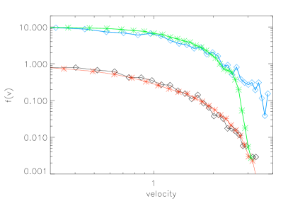
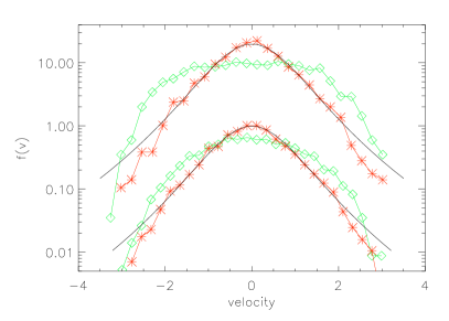
When analyzing dark matter structures resulting from cosmological simulations, we find that the shape of the radial VDF changes as a function of radius (Wojtak et al., 2005; Hansen et al., 2006; Faltenbacher & Diemand, 2006; Fairbairn & Schwetz, 2008). In particular, the bins in the inner region tend to have long tails (more particles at high velocity compared to a Gaussian), whereas bins at larger radii tend to have stronger reduction in high velocity particles. This is exemplified in figure 1, where the upper curves (blue and green) show the radial VDF. The open diamonds (blue) come from a radial bin in the inner region, whereas the stars (green) are from a bin further out. The VDF’s are normalized such that a comparison is possible, and velocity is normalized to the dispersion. This simulated cosmological data is from the Local Group simulation of Moore et al. (2001). The lower curves (red and black) are the tangential VDF from the same two bins, however, for the tangential VDF there is a striking resemblance, infact to a first approximation these two tangential VDF’s from different radial bins look identical.
The most frequently used approach to discuss DM structures is through the first Jeans equation, which relates the velocity dispersions to the density profiles. If we were to have some knowledge about some of the quantities entering the Jeans equation, then we can solve for the others. One example hereof was presented in Dehnen & McLaughlin (2005), who demonstrated how to derive a generalized NFW density profile, by both assuming that the pseudo phase-space is a power-law in radius (Taylor & Navarro, 2001), and that there is a linear relation between the velocity anisotropy and the density slope (Hansen & Moore, 2006). A somewhat generalized approach was presented in Zait et al. (2008), where the authors demonstrated how to derive the velocity anisotropy by assuming simple forms for both the density profile and the pseudo phase-space density. The fundamental problem with this kind of approaches is, that any departure from truth in the assumptions will lead to departure from correctness in the results. Zait et al. (2008) demonstrated this in a very convincing way, by deriving significantly different velocity anisotropy profiles by just changing between NFW or Sersic density profiles as input. Another related problem with these approaches is, that the assumption that pseudo phase-space is a simple power-law, was recently demonstrated to be oversimplified. The unknown question was which component (radial, tangential, or something else) of the velocity dispersion in the pseudo phase-space gives the best approximation to a power-law in radius (Hansen et al., 2006; Knollmann et al., 2008). Schmidt et al. (2008) demonstrated that different numerically simulated structures are best fitted by different forms of the pseudo phase-space, and hence that there is no universal simple behavior of the pseudo phase-space.
2.1 The shape of the radial VDF
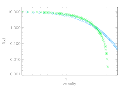
For ergodic structures, that is structures where the orbits depend only on energy (hence with ) we can use the Eddington formula to get the VDF at any radius (Eddington, 1916), (see also Binney (1982); Cuddeford (1991); Evans & An (2006)). The Eddington formula only depends on the radial dependence of the density profile of the structure, and by assumption the VDF is the same for the radial and tangential directions, function. It is natural to interpret this in the following way. The structure is in equilibrium, so there is detailed balance for each phase-space element. The velocity of each particle is decomposed into the radial and tangential components, and for any infinitesimal time step, the radial component of any individual particle can tell that it is moving in a changing density and changing potential (the radial component of any individual particle is either moving directly inwards or outwards). It is therefore natural that the radial VDF is imprinted by the radial variation in the density and potential. For a truncated NFW density profile we can e.g. get the VDF at radius 0.1 and 10, in units of the characteristic radius, see figure 2. By comparison of figures 1 and 2 it is clear, that the radial VDF of the cosmological simulation indeed looks very similar to the VDF from the Eddington formula. It is therefore tempting to suggest that the radial VDF to a first approximation is identical to the one which results when applying the Eddington formula to the given density profile.
Now, the actual radial VDF (for a given cosmologically simulated structure) will differ slightly from the VDF resulting from the Eddington formula, since the latter was based on the assumption that . Specifically, the VDF from the Eddington formula gives also , and to ensure consistency with the Jeans equation, one must have . However, we will here use this VDF as a first approximation to the radial VDF, and we will present a quantitative comparison in a future paper. Recently, Van Hese et al. (2008) showed that for a large class of theoretical model, this is an excellent approximation (see their figure 5).
2.2 The shape of the tangential VDF
It is somewhat less trivial to argue (or claim) the shape of the tangential VDF. For an infinitesimal time step, the tangential component of any individual particle’s velocity is moving in constant density and constant potential (the tangential velocity component of any individual particle is moving, well, tangentially, and we assume spherical symmetry). We still assume that the structure is in equilibrium with no time variation. This means, that as a first approximation the tangential VDF can be thought of as the one resulting from an infinite and homogeneous medium, where both the density and potential is constant everywhere. This argument is similar to the Jeans swindle, where the homogeneous medium implies constant potential. Naturally, such an infinite structure is not gravitationally stable against perturbations, but we can instead approximate it in the following way.
Let us consider a density profile, which is a power-law in radius over many orders of magnitude, and is then truncated. One example hereof is an NFW profile, where the central density slope is -1, and the corresponding truncation is then happening after the scale radius. We are thus considering the VDF in a bin at a radius which is many orders of magnitude deeper towards the center than the scale radius. We can now consider a generalized double power-law profile, where the central slope can be more shallow than -1, and we can use the Eddington formula to extract the VDF for any central slope. By lowering the central slope towards zero, we get a structure which in principle is stable towards perturbations, but at the same time is approaching constant density and constant potential in the central region. The resulting VDF (extrapolated to zero slope) has been discussed by Hansen et al. (2005) and has the shape
| (2) |
with , and shows that the normalization only depends on the local density. This form is known as a q-generalized exponential (Tsallis, 1988). For comparison one should note that a simple comparison with polytropes (where ) breaks down, since the normal connection between density and potential, , is not valid for such shallow slopes (Binney & Tremaine, 1987).
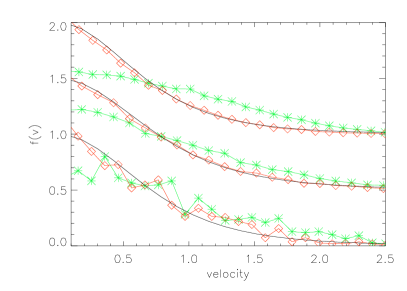
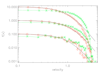
When considering the shape of the tangential VDF from simulations in figs. 3 and 4 we see that this form indeed provides a very good fit for all radii, at least for smaller than roughly . The structure in figs. 3 and 4 is from a very non-cosmological simulation (the “tangential orbit instability” of Hansen et al. (2006)). The same form fits the tangential VDF’s from a cosmological simulation (lower lines in fig. 1) equally well.
Clearly, this form in eq. (2) has an extended tail of high energy particles, which would not be bound by the equilibrated structure. The suppression of high energy particles due to the finite radial extend of the structure is naturally included through the Eddington formula for the radial component, and we therefore make the suggestion that the tangential VDF must have a high-energy tail which follows the radial VDF. Effectively, this means that for large velocities the tangential component of the velocity might as well be moving in the radial direction. This corresponds to the fact that the tangential velocity component of any individual particle actually is moving somewhat radially after a finite time-interval.
When looking at fig. 4 we see that the actual suppression is even slightly larger for these high-energy particles, however, the difference between the suggested and the actual suppression at high energy is very small. When looking at the number of particles (the integral under the curve in fig. 3) we find, that the difference is virtually zero.
In conclusion, the tangential VDF is surprisingly well fit by the phenomenologically predicted shape in eq. (2), and with a high-energy tail suppression corresponding to the tail of the radial VDF.
To emphasize the general nature of the shape of the tangential VDF, we also present the radial and tangential VDF’s of a cosmological simulation of a galaxy, including both cooling gas, star-formation and stars, as well as supernova feedback from Sommer-Larsen et al. (2003); Sommer-Larsen (2006). In fig. 5 we see that the dark matter VDF also in this case has the suggested shape.
3 The velocity anisotropy
Now, after having established the shape of both the radial and tangential VDF’s, the velocity anisotropy at any given radius can easily be determined, as we will show later in this section, since it is just an integral over these distributions, . The shape of the radial VDF changes as a function of radius (section 2.1), whereas the shape of the tangential VDF is virtually constant (section 2.2), and it is therefore natural to expect that the velocity anisotropy will also change as a function of radius. Since the radial VDF generally is more flat-topped than the tangential one (see fig. 4, top lines), then we will expect to be positive. Only when the density slope approaches zero (e.g. a central core) will the radial VDF approach the tangential one, and hence (see fig. 4, bottom lines).
Let us assume that the radial density profile is given, e.g. by a truncated NFW profile. In this case the radial VDF is completely determined through the Eddington formula. The tangential VDF is given by eq. (2) and at first sight there are 2 free parameters, namely the entering equation 2, and then the normalization. For a given we can determine the normalization, since the particle number is conserved when integrating over the radial or tangential VDF, . This leaves us only to determine the entering eq. (2). One could argue that it most likely is either or which should enter here. We will allow ourselves to be guided by the results of numerical simulations, and use the average , since that gives a fairly good approximation to all the tangential VDF’s from the simulations discussed above. We will present a more quantitative test of this in a future paper, but the effect is modest. E.g. for the truncated NFW profile at the radius where the slope is , we find when using , and if we instead use () we get .
It is now straight-forward to calculate the velocity anisotropy, , at any radius for any given density profile with no free parameters. Practically we do it iteratively in the following way. 1) First we find the radial VDF, using the Eddington formula. 2) Then we write the tangential VDF, which is eq. (2) where we initially use (initially assuming to be very small). 3) Then replace this form at high momenta with the radial VDF (as described in detail in section 2), and normalized in such a way that the particle number is conserved (between radial and tangential). 4) It is now trivial to calculate as an integral over these distribution functions, and if this is different from the initial assumption, then re-iterate the entire process with the calculated . This means explicitely that we return to point 2) with this newly calculated , and . In practice we repeat until has converged with accuracy .
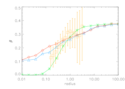
In fig. 6 we present the radial dependence of for 3 density profiles, namely an NFW profile with a truncation at large radius, a profile like the one advocated by Navarro et al. (2004), and finally a profile of the form , which has a central core. We see that the anisotropy increases in a way similar to what is observed in numerical simulations, namely from something small in the central region, to something of the order 0.4 towards the outer region. The orange squares are from CLEF numerial simulation (Kay et al., 2007; Springel, 2005), where the error-bars represent the 1 scatter over the 67 most relaxed clusters (Host et al., 2009). Observations of in galaxy clusters are in excellent agreement with these numerical predictions (Host et al., 2009). The radial scale of the simulated is , which does not have to coincide with the scale radius of the analytical profiles. This gives a free parameter (of the order unity) in the normalization of the x-axis, which we just put to 1 for simplicity. In a similar way the analytical profiles are all normalized to their respective scale radii, which means that they could also have different .
Since we have suggested the shape of the full VDF’s, then we can naturally also get higher order moments, such as the kurtosis, as function of radius. We thus also predict that the radial profile of the higher velocity moments are fully determined by the shape of the density profile.
4 Discussion
One of the consequences of the above considerations is, that the appearance of the radial variation of is dictated by the density profile. That is, given any density profile, the velocity anisotropy is entirely determined, as long as the structure has had time to equilibrate. We are thus stating explicitly, that is unrelated to the infall of matter in the outer region, and that the only connection has to the formation process is through the radial structure of the density profile. This is naturally supported by the very non-cosmological simulations (see figs. 3, 4) which also produce a -profile in agreement with cosmological simulations (Hansen et al., 2006).
Another consequence is that must always be positive in equilibrated structures, since the density profile at most can develop a core (see fig. 6). This is also in good agreement with dark matter simulations (Dehnen & McLaughlin, 2005; Barnes et al., 2007; Faltenbacher & Diemand, 2006; Bellovary et al., 2008). Virtually no numerical simulations find negative velocity anisotropy, and when they do, this is usually only in the very inner region where numerical convergence may be questioned. Few analytical treatments have predicted a negative in the inner region (Zait et al., 2008), however, this result may be an artefact of assuming that the pseudo phases-space is a perfect power-law in radius, which is generally not correct (Schmidt et al., 2008). If future high-resolution numerical simulations instead will establish that the central velocity anisotropy is negative (in agreement with the predictions of Zait et al. (2008)), then that would be a proof that the present analysis is flawed somehow.
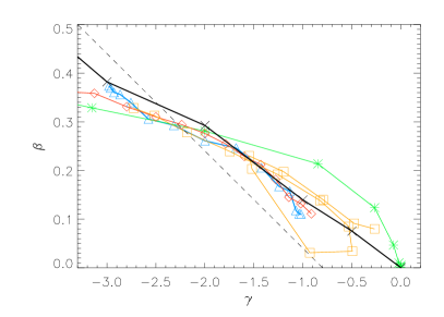
It has previously been suggested that a connection between the anisotropy and the slope of the density profile should exist. This connection appears to hold even for structures which have profiles with non-trivial radial variation in (Hansen & Moore, 2006). We can now test this connection. In figure 7 we show as function of the density slope for the NFW profile (solid line, blue triangles), the profile suggested by Navarro et al. (2004) (red diamonds), and also for a “double-bump” structure (the sum of two spatially separated profiles of the form , orange squares)). This double-hump profile has a very non-trivial radial variation of , which cannot be well approximated by any generalized double power-law profile. All these structures appear to land near a connection roughly given by . We also show the results for the profile (green stars), as well as for single power-law profiles (fat black line, crosses). The dashes line is as suggested in Hansen & Stadel (2006), based on a set of cosmological and non-cosmological simulations. These two results differ by approximately 0.1 in . We indeed see that all structures land in a relatively narrow band in the – plane, and hence likely explaining the origin of the – relations.
The most important practical implication of this suggestion is, that it will allow us to close the Jeans equation. As is well-known, the Jeans equation depends on the density, dispersion, anisotropy and the total mass. Now, having demonstrated (or at least suggested strongly) that the anisotropy is uniquely determined once the density is known, we see that it is possible to close the Jeans equation for systems that are fully relaxed.
We have been making simplifying assumptions above, which all need to be tested through high resolution simulations. First, we assume that the radial VDF is very similar to the one appearing from the Eddington formula, even in the presence of a non-zero . We also assume that the entering eq. (2) is the total one. If the correct to use is instead closer to , then will be slightly larger, but the radial variation will remain. From these assumptions we estimate the accuracy of the present work to be about 0.1 or up to about in .
One could naturally ask why and how the radial and tangential VDF’s get their shapes? It is slightly disappointing that it is not a deep physical principle, like a generalized entropy, which is responsible. Instead it is simply the density profile (either the radially varying, or the tangentially constant) which through the Eddington formula demands that the VDF’s take on these forms. These forms will therefore appear when there is sufficient amount of violent relaxation to allow enough energy exchange between the particles.
5 Summary
The velocity of any particle can be decomposed into the radial and tangential components, and when summing over all particles in a radial bin, we get the particle velocity distribution function, the VDF. We suggest that both the radial and tangential VDF’s are given through the Eddington formula. The radial one comes from the radially changing density profile, and the tangential VDF arises when considering a structure with constant density and potential. This is because the tangential component of the velocity as a first approximation is moving in constant density and constant potential. In addition the tangential VDF is reduced for high-energy particles in accordance with the radial VDF, to ensure that the particles remain bound to the structure. These phenomenological predictions are in remarkably good agreement with the results from numerical simulations of collisionless particles, both of structures of cosmological origin as well as highly non-cosmological origin.
Under these suggestions it is straight forward to derive the velocity anisotropy profile, , with no free parameters. This is shown to increase radially from something small (possibly zero) in the center, to something large and positive (possibly around 0.4) towards the outer region.
We have thus demonstrated that the velocity anisotropy is entirely determined from the density profile. This allows us to close the Jeans equation, since is no-longer a free parameter.
Acknowledgements
It is a pleasure to thank
Jin An and Ole Host for discussions, and Ben Moore and
Jesper Sommer-Larsen for kindly letting me use their
simulations.
The Dark Cosmology Centre is funded by the Danish National Research Foundation.
References
- Ascasibar & Gottloeber (2008) Ascasibar, Y., & Gottloeber, S. 2008, arXiv:0802.4348
- Austin et al. (2005) Austin, C. G., Williams, L. L. R., Barnes, E. I., Babul, A., & Dalcanton, J. J. 2006, ApJ, 634, 756
- Barnes et al. (2007) Barnes, E. I., Williams, L. L. R., Babul, A., & Dalcanton, J. J. 2007, Astrophys. J. 654 (2007) 814
- Bellovary et al. (2008) Bellovary, J. M. et al. 2008, arXiv:0806.3434
- Binney (1982) Binney, J. 1982, MNRAS, 200, 951
- Binney & Tremaine (1987) Binney, J., & Tremaine, S. 1987, Princeton, NJ, Princeton University Press, 1987, 747 p.
- de Blok et al. (2001) de Blok, W. J. G., McGaugh, S. S., Bosma, A., & Rubin, V. C. 2001, ApJ, 552, 23
- de Blok, Bosma & McGaugh (2003) de Blok W. J. G., Bosma A., & McGaugh S. S. 2003, MNRAS, 340, 657
- Broadhurst et al. (2005) Broadhurst, T. J., Takada, M., Umetsu, K., Kong, X., Arimoto, N., Chiba, M., & Futamase, T. 2005, Astrophys. J. 619, L143
- Buote & Lewis (2004) Buote, D. A., & Lewis, A. D. 2004, Astrophys. J. 604, 116
- Carlberg et al. (1997) Carlberg, R. G., et al. 1997, ApJ, 485, L13
- Cole & Lacey (1996) Cole, S., & Lacey, C. 1996, MNRAS, 281, 716
- Corbelli (2003) Corbelli, E. 2003, MNRAS, 342, 199
- Courteau (1997) Courteau, S. 1997, AJ, 114, 2402
- Cuddeford (1991) Cuddeford, P. 1991, MNRAS, 253, 414
- Dehnen & McLaughlin (2005) Dehnen, W., & McLaughlin, D. 2005, MNRAS, 363, 1057
- Diemand et al. (2004) Diemand, J., Moore, B., & Stadel, J. 2004, MNRAS, 353, 624
- Eddington (1916) Eddington, A. S. 1916, MNRAS, 76, 572
- Evans & An (2006) Evans, N. W., & An, J. H. 2006, Phys. Rev. D., 73, 023524
- Fairbairn & Schwetz (2008) Fairbairn, M., & Schwetz, T. 2008, arXiv:0808.0704
- Faltenbacher & Diemand (2006) Faltenbacher,A., & J. Diemand, . 2006, Mon. Not. Roy. Astron. Soc. 369, 1698 [arXiv:astro-ph/0602197].
- Gilmore et al. (2007) Gilmore, G., Wilkinson, M. I., Wyse, R. F. G., Kleyna, J. T., Koch, A., Evans, N. W., & Grebel, E. K. 2007, Astrophys. J. 663, 948
- González-Casado et al. (2007) González-Casado, G., Salvador-Solé, E., Manrique, A., & Hansen, S. H. 2007, arXiv:astro-ph/0702368
- Graham et al. (2006) Graham, A. W., Merritt, D., Moore, B., Diemand, J., & Terzić, B. 2006, AJ, 132, 2701
- Hansen et al. (2005) Hansen, S. H., Egli, D., Hollenstein, L., Salzmann, C. 2005, New Astron. 10, 379
- Hansen & Moore (2006) Hansen S. H., & Moore B 2006, New Astron., 11, 333
- Hansen et al. (2006) Hansen, S. H., Moore, B., Zemp, M., & Stadel, J. 2006, Journal of Cosmology and Astro-Particle Physics, 1, 14
- Hansen & Stadel (2006) Hansen, S. H., & Stadel, J. 2006, Journal of Cosmology and Astro-Particle Physics, 5, 14
- Hansen (2004) Hansen S. H. 2004 MNRAS, 352, L41
- Hansen & Piffaretti (2007) Hansen, S. H., & Piffaretti, R. 2007, A&A, 476, L37
- Host & Hansen (2007) Host, O., & Hansen, S. H. 2007, JCAP, 0706, 016
- Host et al. (2009) Host, O., Hansen, S. H., Piffaretti, R., Morandi, A., Ettori, S., Kay, S. T., & Valdarnini, R. 2009, ApJ to appear, arXiv:0808.2049
- Henriksen (2007) Henriksen, R. N. 2007, arXiv:0709.0434
- Henriksen (2008) Henriksen, R. N. 2008, submitted to ApJ
- Kay et al. (2007) Kay, S. T., da Silva, A. C., Aghanim, N., Blanchard, A., Liddle, A. R., Puget, J.-L., Sadat, R., & Thomas, P. A. 2007, MNRAS, 377, 317
- Knollmann et al. (2008) Knollmann, S. R., Knebe, A. & Hoffman, Y. 2008, arXiv:0809.1439
- Merritt et al. (2006) Merritt, D., Graham, A. W., Moore, B., Diemand, J., & Terzić, B. 2006, AJ, 132, 2685
- Moore et al. (1998) Moore, B., Governato, F., Quinn, T., Stadel, J. & Lake G. 1998, ApJ, 499, 5
- Moore et al. (2001) Moore, B., Calcaneo-Roldan, C., Stadel, J., Quinn, T., Lake, G., Ghigna, S., & Governato, F. 2001, Phys. Rev. D., 64, 063508
- Navarro et al. (1996) Navarro, J. F., Frenk, C. S., & White, S. D. M. 1996, ApJ, 462, 563
- Navarro et al. (2004) Navarro, J. et al. 2004, MNRAS, 349, 1039
- Navarro et al. (2008) Navarro, J. F., et al. 2008, arXiv:0810.1522
- Palunas & Williams (2000) Palunas, P., & Williams, T. B. 2000, AJ, 120, 2884
- Pointecouteau et al. (2005) Pointecouteau, E., Arnaud, M., & Pratt, G. W. 2005, Astron. & Astrophys, 435, 1
- Reed et al. (2003) Reed, D. et al. 2003, Mon. Not. Roy. Astron. Soc. 357, 82
- Rubin et al. (1985) Rubin, V. C., Burstein, D., Ford, W. K., & Thonnard, N. 1985, ApJ, 289, 81
- Salvador-Sole et al. (2007) Salvador-Solé, E., Manrique, A., González-Casado, G., & Hansen, S. H. 2007, ApJ, 666, 181
- Salucci (2001) Salucci, P. 2001, MNRAS, 320L, L1
- Salucci et al. (2003) Salucci, P., Walter, F., & Borriello, A. 2003, A&A, 409, 53
- Salucci et al. (2007) Salucci, P., Lapi, A., Tonini, C., Gentile, G., Yegorova, I., & Klein, U. 2007, MNRAS, 378, 41
- Sand et al. (2004) Sand, D. J., Treu, T., Smith, G. P., & Ellis, R. S. 2004, Astrophys. J. 604, 88
- Schmidt et al. (2008) Schmidt, K., Hansen, S. H., An, J. H., Williams, L. L. R., & Maccio, A. V. 2008, submitted to ApJ
- Schmidt et al. (2008) Schmidt, K. B., Hansen, S. H., & Macciò, A. V. 2008, ApJ, 689, L33
- Sommer-Larsen (2006) Sommer-Larsen, J. 2006, ApJ, 644, L1
- Sommer-Larsen et al. (2003) Sommer-Larsen, J., Götz, M., & Portinari, L. 2003, ApJ, 596, 47
- Springel (2005) Springel, V. 2005, MNRAS, 364, 1105
- Stadel et al. (2008) Stadel, J., Potter, D., Moore, B., Diemand, J., Madau, P., Zemp, M., Kuhlen, M., & Quilis, V. 2008, arXiv:0808.2981
- Stoehr (2004) Stoehr, F. 2004, Mon. Not. Roy. Astron. Soc. 365, 147
- Swaters et al. (2002) Swaters, R. A., Madore, B. F., van den Bosch, F. C., & Balcells, M. 2003, ApJ, 583, 732
- Taylor & Navarro (2001) Taylor, J. E., & Navarro, J. F. 2001, ApJ, 563, 483
- Tsallis (1988) Tsallis, C. 1988, J. Stat. Phys., 52, 479
- Van Hese et al. (2008) Van Hese, E., Baes, M., & Dejonghe, H. 2008, arXiv:0809.0901
- Vikhlinin et al. (2006) Vikhlinin, A., Kravtsov, A., Forman, W., Jones, C., Markevitch, M., Murray, S. S., & Van Speybroeck, L. 2006, Astrophys. J. 640, 691
- Wilkinson et al. (2004) Wilkinson, M. I. et al. 2004, Astrophys. J. 611, L21
- Wojtak et al. (2005) Wojtak, R. et al. Lokas, E. L., Gottloeber, S., & Mamon, G. A. 2005, Mon. Not. Roy. Astron. Soc. 361, L1
- Wojtak et al. (2008) Wojtak, R., Lokas, E. L., Mamon, G. A., Gottloeber, S., Klypin, A., & Hoffman, Y. 2008, arXiv:0802.0429
- Zait et al. (2008) Zait, A., Hoffman, Y., & Shlosman, I. 2008, arXiv:0711.3791