Mistuning-based Control Design to Improve Closed-Loop Stability of Vehicular Platoons
Abstract
We consider a decentralized bidirectional control of a platoon of identical vehicles moving in a straight line. The control objective is for each vehicle to maintain a constant velocity and inter-vehicular separation using only the local information from itself and its two nearest neighbors. Each vehicle is modeled as a double integrator. To aid the analysis, we use continuous approximation to derive a partial differential equation (PDE) approximation of the discrete platoon dynamics. The PDE model is used to explain the progressive loss of closed-loop stability with increasing number of vehicles, and to devise ways to combat this loss of stability.
If every vehicle uses the same controller, we show that the least stable closed-loop eigenvalue approaches zero as in the limit of a large number () of vehicles. We then show how to ameliorate this loss of stability by small amounts of “mistuning”, i.e., changing the controller gains from their nominal values. We prove that with arbitrary small amounts of mistuning, the asymptotic behavior of the least stable closed loop eigenvalue can be improved to . All the conclusions drawn from analysis of the PDE model are corroborated via numerical calculations of the state-space platoon model.
I Introduction
We consider the problem of controlling a one-dimensional platoon of identical vehicles where the individual vehicles move at a constant pre-specified velocity with an inter-vehicular spacing of . Figure 1(a) illustrates the situation schematically. This problem is relevant to automated highway systems (AHS) because a controlled vehicular platoon with a constant but small inter-vehicular distance can help improve the capacity (measured in vehicles/lane/hour, as in [1]) of a highway [2]. Due to this, the platoon control problem has been extensively studied [3, 4, 5, 1, 6, 7]. The dynamic and control issues in the platoon problem are also relevant to a general class of formation control problems including aerial vehicles, satellites etc. [8, 9].
Several approaches to the platoon control problem have been considered in the literature. These approaches fall into two broad categories depending on the information architecture available to the control algorithm(s): centralized and decentralized. We call an architecture decentralized if the control action at any individual vehicle is computed based upon measurements obtained by on-board sensors and possibly wireless communication with a limited number of its neighbors. We call all other architectures centralized. Decentralized architectures investigated in the literature include the predecessor-following [1, 10, 11] and the bidirectional schemes [12, 7, 13, 14, 15]. In the predecessor-following architecture, the control action at an individual vehicle depends only on the spacing error with the predecessor, i.e., the vehicle immediately ahead of it. In the bidirectional architecture, the control action depends upon relative position measurements from both the predecessor and the follower. On the other hand, in a centralized architecture measurements from all the vehicles may have to be continually transmitted to a central controller or to all the vehicles. The optimal QR designs of [4, 6] typically lead to centralized architectures. Predecessor and Leader follower control schemes (see [16, 17] and references therein), which require global information from the first vehicle in the platoon are also examples of the centralized architecture. The high communication overhead in a centralized architecture makes it less attractive for platoons with a large number of vehicles. Additionally, with any centralized scheme, the closed loop system becomes sensitive to communication delays that are unavoidable with wireless communication [18].
The focus of this paper is on a decentralized bidirectional control architecture: the control action at an individual vehicle depends upon its own velocity and the relative position errors between itself and its predecessor and its follower vehicles. The decentralized bidirectional control architecture is advantageous because, apart from its simplicity and modularity, it does not require continual inter-vehicular communication. Measurements needed for the control can be obtained by on-board sensors alone. Each vehicle is modeled as a double integrator. A double integrator model is common in the platoon control literature since the velocity dependent drag and other non-linear terms can usually be eliminated by feedback linearization [1, 10]. The control objective is to maintain a constant inter-vehicular spacing.
In spite of the advantages over centralized control, there are a number of challenges in the decentralized control of a platoon, especially when the number of vehicles, , is large. First, the least stable closed-loop eigenvalue approaches zero as the number of vehicles increases [19]. Among decentralized schemes, one particularly important special case is the so-called symmetric bidirectional control, where all vehicles use identical controllers that are furthermore symmetric with respect to the predecessor and the follower position errors. In this case, the least stable closed loop eigenvalue approaches as with a symmetric bidirectional control and this behavior is independent of the choice of controller gains [19]. This progressive loss of closed-loop damping causes the closed loop performance of the platoon to become arbitrarily sluggish as the number of vehicles increases. It is interesting to note that the decay of the least stable eigenvalue occurs with the centralized LQR control as well [6].
The second challenge with decentralized control is that the sensitivity of the closed loop to external disturbances increases with increasing . With predecessor following control, disturbances acting on the vehicles cause large inter-vehicular spacing errors [3, 1, 20] The seminal work of [20] on string instability was partly inspired by this issue. It was shown in [7] that sensitivity to disturbances with predecessor following control is independent of the choice of the controller. Similar controller-independent sensitivity to disturbances is also exhibited by the symmetric bidirectional architecture [7, 13, 21]. In [22], it was shown that symmetric architectures have similarly poor sensitivity even when every vehicle uses information from more than two neighbors, as long as the number of neighbors is no more than .
Third, there is a lack of design methods for decentralized architectures. For vehicles, in general, distinct controllers need to be designed, for which few control design methods exist. This has led to the examination of only the symmetric control among bidirectional architectures [7, 13, 22]. Some symmetry aided simplifications are possible for analysis and design in this case.
In summary, while issues such as stability and sensitivity to disturbances become critical as the platoon size increases, a lack of analysis and control design tools in decentralized settings makes it difficult to address these issues.
In this paper we present a novel analysis and design method for a decentralized bidirectional control architecture that ameliorates the progressive loss of closed loop stability with increasing number of vehicles. There are three contributions of this work that are summarized below.
First, we derive a partial differential equation (PDE) based continuous approximation of the (spatially) discrete platoon dynamics. Just as a PDE can be discretized using a finite difference approximation, we carry out a reverse procedure: spatial difference terms in the discrete model are approximated by spatial derivatives. The resulting PDE yields the original set of ordinary differential equations upon discretization.
Two, we use the PDE model to derive a controller independent conclusion on stability with symmetric bi-directional architecture. In particular, the behavior of the least stable eigenvalue of the discrete platoon dynamics is predicted by analyzing the eigenvalues of the PDE. We show that the least stable closed-loop eigenvalue approaches zero as . This prediction is confirmed by numerical evaluation of eigenvalues for both the PDE and the discrete platoon model. The real part of the least stable eigenvalue of the closed loop is taken as a measure of stability margin.
The third and the main contribution of the paper is a mistuning-based control design that leads to significant improvement in the closed loop stability margin over the symmetric case. The biggest advantage of using a PDE-based analysis is that the PDE reveals, better than the state-space model does, the mechanism of loss of stability and suggests a mistuning-based approach to ameliorate it. In particular, analysis of the PDE shows that forward-backward asymmetry in the control gains is beneficial. The asymmetry refers to the assignment of controller gains such that a vehicle utilizes information from the preceding and following vehicles differently. Our main results, Corollary 2 and Corollary 3, give control gains that achieve the best improvement in closed-loop stability by exploiting this asymmetry. In particular, we show that an arbitrarily small perturbation (asymmetry) in the controller gains from their values in the symmetric bidirectional case can result in the least stable eigenvalue approaching only as (as opposed to in the symmetric bidirectional case). Numerical computations of eigenvalues of the state-space model of the platoon is used to confirm these predictions. Mistuning based approaches have been used for stability augmentation in many applications; see [23, 24, 25, 26] for some recent references. Our paper is the first to consider such approaches in the context of decentralized control design.
Although the PDE model is derived under the assumption of large , in practice the predictions of the PDE model match those of the state-space model accurately even for small values of . Similarly, the benefits of mistuning are significant even for small values of (see Section VI).
In addition to the stability margin improvements, the mistuning design reduces the closed loop’s sensitivity to external disturbances as well. In bidirectional architectures, the norm of the transfer function from the external disturbances to the spacing errors is used as a measure of sensitivity to disturbances [7]. Numerical computation of the norm of this transfer function shows that mistuning design also reduces sensitivity to disturbances significantly (see Section VI-D).
We briefly note that there is an extensive literature on modeling traffic dynamics using PDEs; see the seminal paper of Lighthill and Whitham [27] for an early reference, the paper of Helbing [28] and references therein for a survey of major approaches, and the papers of [29] and [30] for control-oriented modeling. In spite of apparent similarities, our approach is quite different from the existing approaches. PDE models of traffic dynamics typically start with continuity and momentum equations [28]. Moreover, one requires a model of human behavior to determine an appropriate form of the external force in the momentum equation. This difficulty frequently leads to the introduction of terms in the PDE that are determined by fitting data; see [28, Section III-D] for a thorough discussion of such approximations used in various continuum traffic models. In contrast, we approximate the closed loop dynamic equations by continuous functions of space (and time) that are inspired by finite-difference discretization of PDEs. Ad-hoc approximations of human behavior is not needed. Moreover, the original dynamics can be recovered by discretizing the derived PDE, which provides further evidence of consistency between the (spatially) discrete and continuous models.
We also note that macroscopic models of traffic flow models have been used for designing control laws for a complete automated highway system (AHS) with lane changing, merging, etc. in addition to a platoon in one lane (see [30, 31] and references therein). The PDE model derived in the paper is not applicable to a complete AHS, but only to a single platoon.
The rest of the paper is organized as follows: section II states the platoon problem in formal terms by describing a state-space model of the closed loop platoon dynamics; section III then describes the derivation of the PDE model from the state space model. In section IV the PDE is analyzed to explain the loss of stability with , and section V describes how to ameliorate such loss of stability by mistuning. Section V-C reports simulation results that show the benefit of mistuning in time-domain. In Section VI, we comment on various aspects of the proposed mistuning design.
II Closed loop dynamics with bidirectional control
Consider a platoon of identical vehicles moving in a straight line as shown schematically in Figure 1(a). Let and denote the position and the velocity, respectively, of the vehicle for . Each vehicle is modeled as a double integrator:
| (1) |
where is the control (engine torque) applied on the vehicle. Such a model arises after the velocity dependent drag and other non-linear terms have been eliminated by using feedback linearization [1, 10].
The control objective is to maintain a constant inter-vehicular distance and a constant velocity for every vehicle. Every vehicle is assumed to know the desired spacing and the desired velocity . The control architecture is required to be decentralized, so that every vehicle uses locally available measurements. We assume that the error between the position (as well as velocity) of a vehicle and its desired value is small, so that analysis of the platoon dynamics with a linear vehicle model and a linear control law is justified.
| Scenario | Length | Leader | Follower |
|---|---|---|---|
| I | |||
| II | – |
In this paper, we assume a bi-directional control architecture for individual vehicles in the platoon (except the first and the last vehicles). For the first and the last vehicles, we consider two types of control architectures (termed as scenarios I and II) as tabulated in Table I. In scenario I, we introduce (after [6, 5]) a fictitious lead vehicle and a fictitious follow vehicle, indexed as and respectively. Their behavior is specified by imposing a constant velocity trajectories as and . In scenario II, only a fictitious lead vehicle with index with is introduced. For the last vehicle in the platoon in scenario II, there is no follower vehicle and it uses information only from its predecessor to maintain a constant gap.
Consistent with the decentralized bidirectional linear control architecture, the control for the vehicle is assumed to depend only on 1) its velocity error , and 2) the relative position errors between itself and its immediate neighbors. That is,
| (2) |
where are positive constants. The first two terms are used to compensate for any deviation away from nominal position with the predecessor (front) and the follower (back) vehicles respectively. The superscripts (f) and (b) correspond to front and back, respectively. The third term is used to obtain a zero steady-state error in velocity. In principle, relative velocity errors between neighboring vehicles can also be incorporated into the control, but we do not examine this situation here. Since and are known to every vehicle, the relative errors used in the control law, including the velocity error, can be obtained in practice by on-board devices such as radars, GPS, and speed sensors.
The control law (2) represents state feedback with local (nearest neighbor) information. Analysis of this controller structure is relevant even if there are additional dynamic elements in the controller. There are several reasons for this. First, a dynamic controller cannot have a zero at the origin. It will result in a pole-zero cancellation causing the steady-state errors to grow without bound as increases [13]. Second, a dynamic controller cannot have an integrator either. For if it does, the closed-loop platoon dynamics become unstable for a sufficiently large values of [13]. As a result, any allowable dynamic compensator must essentially act as a static gain at low frequencies. The results of [13] indicate that the principal challenge in controlling large platoons arises due to the presence of a double integrator with its unbounded gain at low frequencies. Hence, the limitation and its amelioration discussed here with the local state feedback structure of (8) is also relevant to the case where additional dynamic elements appear in the control.
To facilitate analysis, we consider a coordinate change
| (3) |
where denotes the desired platoon length, which equals in scenario I and in scenario II. Figure 1(b) depicts the schematic of the platoon in the new coordinates. The scaling ensures that , , and () in scenario I (II). Here, we have implicitly assumed that deviations of the vehicle positions and velocities from their desired values are small.
In the scaled coordinate, the dynamics of the vehicle are described by
| (4) |
where . The desired spacing and velocities are
| (5) |
and the desired position of the vehicle is
| (6) |
The position and velocity errors for the vehicle are given by:
| (7) | ||||
We note that for the fictitious lead and follow vehicles. In the scaled coordinates, the decentralized bidirectional control law (2) is equivalent to the following
| (8) | ||||
It follows from (4) and (8) that the closed loop dynamics of the vehicle in the -coordinate is
| (9) |
To describe the closed-loop dynamics of the whole platoon, we define
For scenario I with fictitious lead and follow vehicles, the control law (8) yields the following closed loop dynamics.
| (10) |
where , , , and
For scenario II with a fictitious lead vehicle and no follow vehicle, the closed loop dynamics are
| (11) |
where , , and
Our goal is to understand the behavior of the closed loop stability margin with increasing and to devise ways to improve it by appropriately choosing the controller gains. While in principle this can be done by analyzing the eigenvalues of the matrix (scenario I) and of (scenario II), we take an alternate route. For large values of , we approximate the dynamics of the discrete platoon by a partial differential equation (PDE) which is used for analysis and control design.
III PDE model of platoon closed loop dynamics
In this section, we develop a continuous PDE approximation of the (spatially) discrete platoon dynamics. The PDE is derived with respect to a scaled spatial coordinate . We recall that in Section II, the scaled location of the vehicle (denoted as ) was defined with respect to such a coordinate system. In effect, the two symbols and correspond to the same coordinate representation but are used here to distinguish the continuous and discrete formulations. As in the discrete case, the platoon always occupies a length of irrespective of .
III-A PDE derivation
The starting point is a continuous approximation:
Similarly, are used to denote continuous approximations of discrete gains respectively. We will construct a PDE approximation of discrete dynamics in terms of these continuous approximations. To do so, it is convenient to first differentiate (9) with respect to time,
| (12) |
We recast this equation
where
| (13) |
It follows that
where
| (14) |
has the physical interpretation of the mean density (vehicles per unit length). Now, we make a finite-difference approximation of derivatives
where we recall that is a continuous approximation of the vehicle velocities ( etc). Denoting and as continuous approximations of and respectively, the discrete model is written as:
Hence, we arrive at the partial differential equation (PDE) as a model of the discrete platoon dynamics:
| (15) |
In the remainder of this paper, we assume that . Using (13), the continuous counterparts of the front and the back gains are given by
| (16) | ||||
so that the gain values can be obtained as and . It can be readily verified that one recovers the system of ordinary differential equations ((12) for ) by discretizing the PDE (15) using a finite difference scheme on the interval with a discretization between discrete points.
The boundary conditions for the PDE (15) depend upon the dynamics of the first and the last vehicles in the platoon. For scenario I with a constant velocity fictitious lead and follow vehicles, the appropriate boundary conditions are of the Dirichlet type on both ends:
| (17) |
For scenario II with the only a fictitious lead vehicle, the appropriate boundary conditions are of Neumann-Dirichlet type:
| (18) |
We refer the reader to Appendix A-A for a discussion on well-posedness of the solutions to (15). It is shown in Appendix A-A that a solution exists in a weak sense when .
Equation (15) describes spatio-temporal evolution of small velocity perturbations in a platoon. It is worthwhile to note that the PDE model is a hyperbolic equation. Without the two first order terms (i.e., for ), the PDE is a standard wave equation with spatially inhomogeneous values of wave speed. The term is an advection term, and is a damping term. The hyperbolic nature of the PDE model means that a perturbation originating, say, in the middle of a long platoon will propagate both upstream and downstream with finite speed. The two first order terms serve to modify aspects of this propagation. The damping term causes a perturbation to damp out in time. The advection term serves to create possible asymmetries in upstream versus downstream propagation.
III-B Eigenvalue comparison
For preliminary comparison of the PDE obtained above with the state-space model of the closed loop platoon dynamics, we consider the simplest case where the position control gains are constant for every vehicle, i.e., and . In such a case , and the PDE (15) simplifies to
| (19) |
which is a damped wave equation with a wave speed of . The wave equation is consistent with the physical intuition that a symmetric bidirectional control architecture causes a disturbance to propagate equally in both directions.
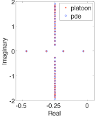
Figure 2 compares the closed loop eigenvalues of a discrete platoon with vehicles and the PDE (19). The eigenvalues of the platoon are obtained by numerically evaluating the eigenvalues of the matrices and (defined in (10) and (11)). The eigenvalues of the PDE are computed numerically after using a Galerkin method with Fourier basis [32]. The figure shows that the two sets of eigenvalues are in excellent match. In particular, the least stable eigenvalues are well-captured by the PDE. Additional comparison appears in the following sections, where we present the results for analysis and control design.
IV Analysis of the symmetric bidirectional case
This section is concerned with asymptotic formulas for stability margin (least stable eigenvalue) for the symmetric bidirectional architecture with symmetric and constant control gains: and . The analysis is carried out with the aid of the associated PDE model:
| (20) |
where and
| (21) |
is the wave speed. The closed-loop eigenvalues of the PDE require consideration of the eigenvalue problem
| (22) |
where is an eigenfunction that satisfies appropriate boundary conditions: (17) for scenario I and (18) for scenario II. The eigensolutions to the eigenvalue problem (23) for the two scenarios are given in Table II. The eigenfunctions in either scenario provide a basis of .
| boundary condition | eigenvalue | eigenfunction | |
|---|---|---|---|
| (Dirichlet - Dirichlet) | |||
| (Neumann - Dirichlet) |
After taking a Laplace transform, the eigenvalues of the PDE model (20) are obtained as roots of the characteristic equation
| (23) |
where satisfies (22). Using Table II, these roots are easily evaluated. For instance, the eigenvalue of the PDE (20) with Dirichlet boundary conditions is given by
| (24) |
where . The real part of the eigenvalue depends upon the discriminant , where the wave speed depends both on control gain and number of vehicles (see (21)). For a fixed control gain, there are two cases to consider:
-
1.
If , the roots are complex with the real part given by ,
-
2.
If , the roots are real with .
In the former case, the damping is determined by the velocity feedback term , while in the latter case one eigenvalue () gains damping at the expense of the other () which looses damping. When are real, the eigenvalue is closer to the origin than ; so we call the less-stable eigenvalue. The following lemma gives the asymptotic formula for this eigenvalue in the limit of large .
Lemma 1
| boundary condition | for | |
|---|---|---|
| Dirichlet-Dirichlet | ||
| Neumann-Dirichlet |
- Proof of Lemma 1.
The stability margin of the platoon can be measured by the real part of , the least stable eigenvalue.
Corollary 1
The result shows that the least stable eigenvalue of the closed loop platoon decays as with symmetric bidirectional control.
We now present numerical computations that corroborates this PDE-based analysis. Figure 3 plots as a function of the least stable eigenvalue of the PDE and of the state-space model of the platoon, as well as the prediction from the asymptotic formula. The eigenvalues for the discrete platoon are obtained by numerically evaluating the eigenvalues of the matrices and (see (10) and (11)) with constant control gains and for . The comparison shows that the PDE analysis accurately predicts the eigenvalue of the state-space model of the platoon dynamics.
Figure 4(a) graphically illustrates the destabilization by depicting the movement of eigenvalues as increases. For sufficiently small values of , the discriminant is negative and the eigenvalue are complex. The real part of the eigenvalue depends only on the value of . At a critical value of , the discriminant becomes zero, and the eigenvalues collide on the real axis. For values of and in particular as , the eigenvalue asymptotes to while staying real, and asymptotes to . Their cumulative damping, as reflected in the sum , is conserved. In other words, is destabilized at the expense of .
Remark 1
The preceding analysis shows that the loss of stability experienced with a symmetric bidirectional architecture is controller independent. The least stable eigenvalue approaches as irrespective of the values of the gains and , as long as they are fixed constants independent of . Corollary 1 also implies that for the least stable eigenvalue to be uniformly bounded away from , one has to increase the control gain as . In [6], the same conclusion was reached for the least stable eigenvalue with LQR control of a platoon on a circle. LQR control typically leads to a centralized architecture, whereas symmetric bidirectional control is decentralized. It is interesting to note that the least stable eigenvalue behaves similarly in these distinct architectures.
V Reducing loss of stability by mistuning
In this section, we examine the problem of designing the control gain functions so as to ameliorate the loss of stability margin with increasing that was seen in the previous sections when . Specifically, we consider the eigenvalue problem for the PDE (15) where the control gains are changed slightly (mistuned) from their values in the symmetric bidirectional case in order to minimize the least-stable eigenvalue . With symmetric bidirectional control, one obtains an estimate for the least stable eigenvalue because the coefficient of term in PDE (15) is and the coefficient of term is . Any asymmetry between the forward and the backward gains will lead to non-zero and a presence of term as coefficient of . By a judicious choice of asymmetry, there is thus a potential to improve the stability margin from to .
We begin by considering the forward and backward position feedback gain profiles:
where is a small parameter signifying the amount of mistuning and , are functions defined over the interval that capture perturbation from the nominal value . Define
so that from (16),
The mistuned version of the PDE (15) is then given by
| (28) |
We study the problem of improving the stability margin by judicious choice of and . The results of our investigation, carried out in the following sections, provide a systematic framework for designing control gains in the platoon by introducing small changes to the symmetric design.
V-A Mistuning-based design for scenario I
The control objective is to design mistuning profiles and to minimize the least stable eigenvalue . To achieve this, we first obtain an explicit asymptotic formula for the eigenvalues when a small amount of asymmetry is introduced in the control gains (i.e., when is small). For scenario I, the result is presented in the following theorem. The proof appears in Appendix A-B.
Theorem 1
It is apparent from the Theorem above that to minimize the least stable eigenvalue , one needs to choose only carefully; has only effect. Therefore we choose , or, equivalently, , which leads to . The most beneficial control gains are now can be readily obtained from Theorem 1, which is summarized in the next corollary.
Corollary 2 (Mistuning profile for Scenario I)
Consider the problem of minimizing the least-stable eigenvalue of the PDE (28) with Dirichlet boundary condition (17) by choosing with norm-constraint and . In the limit as , the optimal mistuning profile is given by , where is the Heaviside function: for and for . With this profile, the least stable eigenvalue is given by the asymptotic formula
in the limit as and .
The result shows that even with an arbitrarily small amount of mistuning , one can improve the closed-loop platoon damping by a large amount, especially for large values of . The least-stable eigenvalue asymptotes to as in the mistuned case as opposed to in the symmetric case.
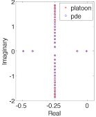
Figure 5(a) shows the gains for the individual vehicles (that are obtained from sampling the functions and ), suggested by Corollary 2 for a vehicle platoon, with and :
where is the desired inter-vehicular spacing in the scaled coordinates, and is defined in (5). A confirmation of the predictions of Corollary 2 is presented in Figure 6. Numerically obtained mistuned and nominal eigenvalues for both the PDE and the platoon state-space model are shown in the figure, with mistuned gains chosen as shown in Figure 5(a). The figure shows that
-
1.
the platoon eigenvalues match the PDE eigenvalues accurately over a range of , and
-
2.
the mistuned eigenvalues show large improvement over the nominal case even though the controller gains differ from their nominal values only by . The improvement is particularly noticeable for large values of , while being significant even for small values of .
For comparison, the figure also depicts the asymptotic eigenvalue formula given in Corollary 2.
Figure 4(b) graphically illustrates the mechanism by which mistuning affects the movement of eigenvalues as increases. By properly choosing the mistuning patterns and , damping can be “exchanged” between the eigenvalues and so that the less stable eigenvalue “gains” stability at the expense of the more stable eigenvalue . The net amount of damping is preserved, since (as seen from Theorem 1).
V-B Mistuning-based design for scenario II
For scenario II, asymptotic formula for the eigenvalue (counterpart of Theorem 1) is summarized in the following theorem. The proof is entirely analogous to the proof of Theorem 1, and is therefore omitted.
Theorem 2
As with scenario I, here again we use the above result to determine the most beneficial profile for small :
Corollary 3 (Mistuning profile for Scenario II)
Consider the problem of minimizing the least-stable eigenvalue of the PDE (28) with Neumann-Dirichlet boundary conditions (18) by choosing with norm-constraint , and . In the limit as , the optimal is given by . With this profile, the least-stable eigenvalue is given by the asymptotic formula
in the limit as and .
The result shows that, as in scenario I, it is possible to improve the closed-loop stability margin in scenario II with an arbitrary small amount of mistuning such that the least-stable eigenvalue asymptotes to as in the mistuned case as opposed to in the symmetric case. The gains suggested by Corollary 3, with and are:
| and |
which are shown in Figure 5(b). Numerically obtained least stable eigenvalues for the PDE and the platoon state-space model for scenario II are shown in Fig. 7 for a range of values of . It is clear from the figure that, as in scenario I, the mistuned eigenvalues show an order of magnitude improvement over their values in the symmetric bidirectional case with only variation.
Remark 2 (Robustness to small changes from the optimal gains)
An advantage of the mistuning design is that mistuned closed loop eigenvalues are robust to small local discrepancies in the control gains from the optimal ones. This can be seen (for scenario I) from the asymptotic eigenvalue formulas of Theorem 1, which shows that one would obtain a estimate for any choice of such that . A similar argument holds for scenario II.
V-C Simulations
We now present results of a few simulations that show the time-domain improvements – manifested in faster decay of initial errors – with the mistuning-based design of control gains. Simulations were carried out for a platoon of vehicles with scenario I, i.e., with fictitious lead and follow vehicles. The desired gap was and desired velocity was . The initial velocity of every vehicle was chosen as the desired velocity and the initial position of the vehicle was chosen as for . As a result, the initial relative position error and velocity error of every vehicle was zero except for the first vehicle, whose relative position error with respect to the fictitious lead vehicle was .
Figure 8 shows the time-histories of the absolute and relative position errors of the individual vehicles with a symmetric bidirectional control, where the control gains were chosen as and for . The absolute position error of the vehicle is and the relative position error is .
Figure 9 shows the time-histories of the absolute and relative position errors for the platoon with mistuned controller gains. The mistuning gains used for the simulation are the ones shown in Figure 5(a) (chosen according to Corollary 2) so that maximum and minimum gains over all vehicles is within of the nominal value. On comparing Figures 8 and 9, we see that the errors in the initial conditions are reduced faster in the mistuned case compared to the nominal case. These observations are consistent with the improvement in the closed-loop stability margin with the mistuned design.
VI Discussion on mistuning design
There are several remarks to be made regarding the mistuning based design. We first comment on the implementation issues, in particular, on the effect of small platoon size on the proposed design, and on the information requirements for its implementation.
VI-A Large vs. small
The PDE model is developed for large . However, detailed numerical comparison between the PDE and the discrete state space model shows that the PDE model provides quantitatively correct predictions even for small values of (see Figures 3, 6 and 7). The PDE has an infinite number of eigenvalues as opposed to a finite number for the discrete platoon. So, one can not expect an exact match. However, PDE eigenvalues exactly match the least stable and other dominant eigenvalues of the discrete platoon (see Figure 2 and Figure 10). In a similar vein, the benefits of mistuning are also realized for small values of . For example, when the number of vehicles is , a mistuning of results in an improvement in the stability margin – as measured by the real part of the least stable eigenvalue – of (from to ) in scenario I and an improvement of (from to ) in scenario II over the symmetric case.
VI-B Information requirements
In order to implement the beneficial mistuned controller gains designed above, every vehicle needs the following information (in addition to what is needed to use a symmetric bidirectional control): (1) the mistuning amplitude , and (2) in scenario I, whether it is in the front half of the platoon or not. This information can be provided to the vehicles in advance. In scenario II, only the value of is needed.
It is possible that due to vehicles leaving and joining the platoon, information on whether a vehicle belongs to the front half of the platoon may become erroneous with time, especially for the vehicles that are close to the middle. In scenario I, such error may lead to a non-optimal gains used by the vehicles. However, since the improvement in closed loop stability margin due to mistuning is robust to small deviations in the gains from the optimal ones (see Remark 2), errors in determining whether a vehicle belongs to the front half of the platoon or not will not greatly affect the improvement in stability margin. Note that in scenario II this issue does not even arise.
VI-C Large asymmetry
Although the mistuning profiles described in Corollaries 2 and 3 are optimal in the limit as , one would like to be able to use them with somewhat larger values of to realize the benefit of mistuning. To do so, one has to preclude the possibility of “eigenvalue cross-over”, i.e., of the second () or some other marginally stable eigenvalue from becoming the least stable eigenvalue in the presence of mistuning. It turns out that such a cross-over is ruled out as a consequence of the Strum-Liouville (S-L) theory for the elliptic boundary value problems. The standard argument relies on the positivity of the eigenfunction corresponding to ; the reader is referred to [33] for the details. Figure 10 verifies this numerically by depicting the six eigenvalues closest to (for both the PDE and the discrete platoon) as a function of when mistuning is applied.
VI-D Sensitivity to disturbance
Automated platoons suffer from high sensitivity to external disturbances; which is referred to as “string instability” or “slinky-type effects” [20, 1, 15]. Here we provide numerical evidence that mistuning also helps in reducing the sensitivity to disturbances.
When external disturbances are present, we model the dynamics of vehicle by , where is the external disturbance acting on the vehicle. In the coordinates, the vehicle dynamics become , where . In scenario I, the state space model of the entire platoon becomes,
| (29) |
where , , , and is a vector of front spacing errors .
The norm of the transfer function from the disturbance to the inter-vehicle spacing errors is a measure of the closed loop’s sensitivity to external disturbances [7, 13]. Figure 11 shows a plot of the norm of as a function of , with and without mistuning. The mistuning profile used is the same as the one used for the eigenvalue trends reported in Figure 6. It is clear from the figure that mistuning results in large reduction of the norm of . Although this reduction is more pronounced for large , it is still significant for small . In particular, for , a mistuning yields approximately reduction in the norm (from 6.69 to 3.38).
Apart from the norm of , there are other ways to measure sensitivity to disturbances. In [21], the transfer function from disturbance acting on the lead vehicle to spacing error on the vehicle is analyzed. Detailed analysis of the effect of mistuning on sensitivity to disturbances will be a subject of future work.
VII Conclusion
We developed a PDE model that describes the closed loop dynamics of an -vehicle platoon with a decentralized bidirectional control architecture. Analysis of the PDE model revealed several important features of the problem. First, we showed that when every vehicle uses the same controller with constant gain that is independent of (the so-called symmetric bidirectional architecture), the least stable eigenvalue of the closed loop decays to as . Second, and more significantly, analysis of the PDE suggested a way to ameliorate the progressive loss of stability with increasing , by introducing small amounts of “mistuning”, i.e., by changing the controller gains from their nominal symmetric values. We proved that with arbitrary small amounts of mistuning, the decay of the least stable closed loop eigenvalue can be improved to . Several comparisons with the numerically computed eigenvalues of state-space model of the platoon confirm the predictions of the PDE-based analysis.
Although the PDE model is derived under the assumption that the number of vehicles, , is large, in practice the PDE provides quantitatively correct predictions for the discrete platoon dynamics even for relatively small values of . The amount of information that is needed to implement the mistuned control gains (over that in the symmetric bidirectional architecture) is quite small and need to be provided only once. Furthermore, the stability improvement due to mistuning is robust to small errors (between the actual gains used and the optimal mistuned gains) that may occur in practice due to changes in the number of vehicles in the platoon over time.
The advantage of the PDE formulation is reflected in the ease with which the closed loop eigenvalues are obtained for two different boundary conditions, with lead and follow vehicles as well as with only a lead vehicle. Certain important aspects of the problem, such as the beneficial nature of forward-backward asymmetry in control gains, is revealed by the PDE while they are difficult to see with the (spatially) discrete, state-space model.
Numerical calculations show that the mistuning design also reduces sensitivity to disturbances of the closed-loop platoon. Analysis of the beneficial effect of mistuning in reducing sensitivity to external disturbances is a subject of future research. In the future, we also plan to examine PDE-based models for modeling and analysis of fleet of vehicles as in or spatial dimensions.
References
- [1] S. Darbha, J. K. Hedrick, C. C. Chien, and P. Ioannou, “A comparison of spacing and headway control laws for automatically controlled vehicles,” Vehicle System Dynamics, vol. 23, pp. 597–625, 1994.
- [2] J. K. Hedrick, M. Tomizuka, and P. Varaiya, “Control issues in automated highway systems,” IEEE Control Systems Magazine, vol. 14, pp. 21 – 32, December 1994.
- [3] R. E. Chandler, R. Herman, and E. W. Montroll, “Traffic dynamics: Studies in car following,” Operations Research, vol. 6, no. 2, pp. 165–184, Mar. - Apr. 1958.
- [4] W. S. Levine and M. Athans, “On the optimal error regulation of a string of moving vehicles,” IEEE Transactions on Automatic Control, vol. AC-11, no. 3, pp. 355–361, July 1966.
- [5] S. M. Melzer and B. C. Kuo, “A closed-form solution for the optimal error regulation of a string of moving vehicles,” IEEE Transactions on Automatic Control, vol. AC-16, no. 1, pp. 50–52, February 1971.
- [6] M. R. Jovanović and B. Bamieh, “On the ill-posedness of certain vehicular platoon control problems,” IEEE Transactions on Automatic Control, vol. 50, no. 9, pp. 1307 – 1321, September 2005.
- [7] P. Seiler, A. Pant, and J. K. Hedrick, “Disturbance propagation in vehicle strings,” IEEE Transactions on Automatic Control, vol. 49, pp. 1835–1841, October 2004.
- [8] J. D. Wolfe, D. F. Chichkat, and J. L. Speyer, “Decentralized controllers for unmaned aerial vehicle formation flight,” in Guidance, Navigation and Control Conference, 1996, pp. July 29–31.
- [9] P. K. C. Wang, F. Y. Hadaegh, and K. Lau, “Synchronized formation rotation and attitude control of multiple free-flying spacecraft,” Journal of Guidance, Control, and Dynamics, vol. 22, no. 1, pp. 28–35, 1999.
- [10] S. S. Stankovic, M. J. Stanojevic, and D. D. Siljak, “Decentralized overlapping control of a platoon of vehicles,” IEEE Transactions on Control Systems Technology, vol. 8, pp. 816–832, September 2000.
- [11] P. Li and A. Shrivastava, “Traffic flow stability induced by constant time headway policy for adaptive cruise control vehicles,” Transportation Research Part C: Emergent Technologies, vol. 10, pp. 275–301, 2002.
- [12] L. E. Peppard, “String stability of relative-motion PID vehicle control systems,” IEEE Transactions on Automatic Control, pp. 579–581, October 1974.
- [13] P. Barooah and J. P. Hespanha, “Error amplification and distrubance propagation in vehicle strings,” in Proceedings of the 44th IEEE conference on Decision and Control, December 2005.
- [14] K. C. Chu, “Decentralized control of high-speed vehicle strings,” Transportation Science, vol. 8, pp. 361–383, 1974.
- [15] Y. Zhang, E. B. Kosmatopoulos, P. A. Ioannou, and C. C. Chien, “Autonomous intelligent cruise control using front and back information for tight vehicle following maneuvers,” IEEE Transactions on Vehicular Technology, vol. 48, pp. 319–328, January 1999.
- [16] S. E. Shladover, “Longitudinal control of automotive vehicles in close-formation platoons,” Journal of Dynamic systems, Measurements and Control, vol. 113, pp. 302–310, December 1978.
- [17] H.-S. Tan, R. Rajamani, and W.-B. Zhang, “Demonstration of an automated highway platoon system,” in American Control Conference, vol. 3, June 1998, pp. 1823 – 1827.
- [18] X. Liu, S. S. Mahal, A. Goldsmith, and J. K. Hedrick, “Effects of communication delay on string stability in vehicle platoons,” in IEEE International Conference on Intelligent Transportation Systems (ITSC), August 2001.
- [19] P. Barooah, P. G. Mehta, and J. P. Hespanha, “Control of large vehicular platoons: Improving closed loop stability by mistuning,” in The 2007 American Control Conference, July, pp. 4666–4671.
- [20] S. Darbha and J. K. Hedrick, “String stability of interconnected systems,” IEEE Transactions on Automatic Control, vol. 41, no. 3, pp. 349–356, March 1996.
- [21] R. H. Middleton and J. H. Braslavsky, “String instability in classes of linear time invariant formation control with limited communication range,” 2008, submitted for publication. [Online]. Available: http://www.hamilton.ie/rick/publications/StringStability.pdf
- [22] S. K. Yadlapalli, S. Darbha, and K. R. Rajagopal, “Information flow and its relation to stability of the motion of vehicles in a rigid formation,” IEEE Transactions on Automatic Control, vol. 51, no. 8, August 2006.
- [23] B. Shapiro, “A symmetry approach to extension of flutter boundaries via mistuning,” Journal of Propulsion and Power, vol. 14, no. 3, pp. 354–366, 1998.
- [24] O. O. Bendiksen, “Localization phenomena in structural dynamics,” Chaos, Solitons, and Fractals, vol. 11, pp. 1621–1660, 2000.
- [25] A. J. Rivas-Guerra and M. P. Mignolet, “Local/global effects of mistuning on the forced response of bladed disks,” Journal of Engineering for Gas Turbines and Power, vol. 125, pp. 1–11, 2003.
- [26] P. G. Mehta, G. Hagen, and A. Banaszuk, “Symmetry and symmetry breaking for a wave equation with feedback,” SIAM Journal of Dynamical Systems, vol. 6, no. 3, pp. 549–575, 2007.
- [27] M. Lighthill and G. Whitham, “On kinematic waves II: a theory of traffic flow on long crowded roads,” in Royal Society, London Series A, 1955.
- [28] D. Helbing, “Traffic and related self-driven many-particle systems,” Review of Modern Physics, vol. 73, pp. 1067–1141, 2001.
- [29] D. Jacquet, C. C. de Wit, and D. Koenig, “Traffic control and monitoring with a macroscopic model in the presence of strong congestion waves,” in 44th IEEE Conference on Decision and Control & European Control Conference, 2005, pp. 2164–2169.
- [30] P. Y. Li, R. Horowitz, L. Alvarez, J. Frankel, and A. M. Robertson, “An automated highway system link layer controller for traffic flow stabilization,” Transportation Research, Part C, vol. 5, no. 1, pp. 11–37, 1997.
- [31] L. Alvarez, R. Horowitz, and P. Li, “Traffic flow control in automated highway systems,” Control Engineering Practice, vol. 7, pp. 1071–1078, 1999.
- [32] C. Canuto, M. Y. Hussaini, A. Quarteroni, and T. A. Zang, Spectral Methods in Fluid Dynamics, ser. Springer Series in Computational Physics. New York: Springer-Verlag, 1983.
- [33] L. C. Evans, Partial Differential Equations, ser. Graduate Studies in Mathematics. American Mathematical Society, 1998, vol. 19.
- [34] A. Pazy, Semigroups of linear operators and applications to partial differential equations, ser. Applied Mathematical Sciences. New York: Springer-Verlag, 1983, vol. 44.
Appendix A Technical results
A-A Solution properties of PDE (15).
In this section, we use the semigroup theory to obtain results on well-posedness of the PDE (15). To apply these methods, we first re-write the PDE as a first order evolution equation:
| (30) |
where is a linear operator; and . We will assume these coefficients and . has the units of and the physical interpretation of density perturbation.
Using (30), we denote the initial/boundary value problem as:
| (31) |
where , and is defined in (30); and will be assumed to functions in appropriately defined Banach spaces. The main goal of this section will be to show that the solution for the linear problem (30) can be expressed in terms of a semigroup provided eigenvalues of the operator satisfy appropriate bounds. We begin with a discussion of the notation.
Preliminaries and Notation. We denote , denotes the Hilbert space of square integrable functions on (), denotes the Sobolev space of functions such that derivatives up to -order exist in a weak sense and belong to (the Sobolev norm is denoted by ), and denotes the Sobolev space of functions that satisfy the Dirichlet boundary condition. We denote , and equip it with a norm . Let and consider the right hand side of evolution equation (30) as an unbounded but closed densely defined linear operator
| (32) |
A real number belongs to , the resolvent set for , provided the operator is 1-1 and onto. For , the resolvent operator . Finally, we recall that a one-parameter family of linear operators is a -semigroup if 1) for all , 2) for all and , and 3) the mapping is continuous from into . A semigroup is a contraction semigroup if for all . The Hille-Yosida theorem states that a closed densely defined linear operator is the generator of a contraction semigroup if and only if
| (33) |
Our strategy will be to apply Hille-Yosida theorem to deduce solution properties of the evolution equation (31). Following closely the development in [33], there are three steps to accomplish this: 1) we show that is a densely defined closed linear operator on , 2) characterize the resolvent set by considering the eigenvalue problem, and 3) show the bound (33) for the resolvent. Step 2 will lead to an eigenvalue problem, whose analysis and optimization is the subject of this paper. We present details for the three steps next:
-
1.
The domain of , , is dense in because is dense in . To show is closed, consider a sequence such that
(34) (35) where the arrow notation denotes the fact that the convergence is in . Since so , i.e., . Now, is Cauchy in by (34) and is Cauchy in by (35) and
(36) so is Cauchy in and . By repeating essentially the same argument, one also finds that and . Consequently, and .
-
2.
Let , , and consider the operator equation
(37) This is equivalent to two scalar equations
(38) (39) Using the first equation to write , this implies
(40) where
(41) is an elliptic operator (because for all ) and (note that ). Consequently, solutions of ((37)) can be studied in terms of solutions of ((41)). The spectrum of is completely characterized by the spectrum of . We will obtain spectral bounds, dependent upon and , in the following sections. In particular, we will establish that for some and thus . For , its turns out that for any choice of positive (this is also clear from the symmetric eigenvalue problem (41)).
-
3.
If a positive , there exists a unique solution for (38)-(39) via the theory of elliptic operators: solve (40) to obtain and . We write the solution as , define a bilinear form
(42) for and consider an equivalent norm (on ) for solutions as:
(43) To obtain the resolvent bound, we multiply (39) by and use integration by parts:
In general, the bound depends upon . For , we have
where the first inequality holds because and and the last inequality follows from the generalized Cauchy-Schwarz inequality. As a result, and .
For the general case where is not identically zero, one expresses the operator
(44) where
In words, is the operator with and is the operator due to . We note that is a bounded perturbation of (on ). We have already showed the existence of a -semigroup for . For the general operator , the existence follows from using a perturbation theorem (see Theorem 1.1 in Ch. 3 of [34]).
A-B Proof of Theorem 1
-
Proof of Theorem 1.
The spatial inhomogeneity introduced by the -dependent coefficients and destroy the spatial invariance of the nominal PDE (20). Hence, the Fourier basis – eigenfunctions of the Laplacian – no longer lead to a diagonalization of the mistuned PDE. The methods of section IV thus need to be suitably modified. In order to compute the eigenvalues for the mistuned PDE (28), we take a Laplace transform of (28) and get
(45) where is the Laplace transform (with respect to ) of . We are interested in eigenvalues of (45) with Dirichlet boundary conditions, i.e., the values of for which a solution to the homogeneous PDE (45) exists with boundary conditions . To obtain these eigenvalues, we use a perturbation method expressing the eigenfunction and eigenvalue in a series form:
(46) We note that denotes the perturbation to the nominal eigenvalue as a result of the mistuning. Substituting (46) in (45) and doing an balance, we get
(47) whose eigen-solution is given by
where , is an arbitrary real constant, and is given by (24). Next,
Substituting on the left hand side leads to a resonance condition for the right hand side term, denoted by . In particular for a solution to exist, must lie in the range space of the linear operator
(48) For this self-adjoint operator, the range space is the complement of its null space . This gives the resonance condition as
where denotes the standard inner product in . This leads to an equation
(49) For values of , where is given by (24), the equation above leads to an expression for perturbation in the two eigenvalues. We denote these perturbations as . For , we have from from Lemma 1 that when , which happens for every as (see eq. (25)), so that
(50) Note that we have dropped the second integral on the right hand side of (49) because for large . For , for and
(51) Note that
Putting the formulas for the perturbation to the eigenvalues (50) and (51) in (46), we get
Since for (Lemma 1) and , the result follows.