Dynamical Tides in Rotating Planets and Stars

Abstract

Tidal dissipation may be important for the internal evolution as well as the orbits of short-period massive planets—hot Jupiters. We revisit a mechanism proposed by Ogilvie and Lin for tidal forcing of inertial waves, which are short-wavelength, low-frequency disturbances restored primarily by Coriolis rather than buoyancy forces. This mechanism is of particular interest for hot Jupiters because it relies upon a rocky core, and because these bodies are otherwise largely convective. Compared to waves excited at the base of the stratified, externally heated atmosphere, waves excited at the core are more likely to deposit heat in the convective region and thereby affect the planetary radius. However, Ogilvie and Lin’s results were numerical, and the manner of the wave excitation was not clear. Using WKB methods, we demonstrate the production of short waves by scattering of the equilibrium tide off the core at critical latitudes. The tidal dissipation rate associated with these waves scales as the fifth power of the core radius, and the implied tidal $Q$ is of order ten million for nominal values of the planet’s mass, radius, orbital period, and core size. We comment upon an alternative proposal by Wu for exciting inertial waves in an unstratified fluid body by means of compressibility rather than a core. We also find that even a core of rock is unlikely to be rigid. But Ogilvie and Lin’s mechanism should still operate if the core is substantially denser than its immediate surroundings.

1 Introduction

The discovery of extrasolar planets has sharpened the need for a predictive theory of tidal circularization and synchronization. Some $2\%$ of nearby single FGK stars harbor roughly Jupiter-mass planets with orbital periods below ten days (Cumming et al., 2008, and references therein). The orbital eccentricities of the shorter-period planets, especially those below four days, are markedly less than those of the longer period systems, presumably as a result of tidal dissipation (Rasio et al., 1996). Synchronization is likely to occur more easily and at longer periods than circularization because of the smaller moment of inertia associated with the spin as compared to the orbit (Lubow et al., 1997). For close stellar binaries, the lack of an adequate tidal theory causes little uncertainty concerning the internal evolution of the components since tidal heating contributes negligibly to the luminosity, and since it is assumed that tides are always sufficient to synchronize the spins of stars that come into contact with their Roche lobes. The intrinsic luminosities of jovian planets due to their gradual contraction and loss of primordial heat are so small, however, that tidal heating may be competitive. Indeed tides have been invoked to account for the anomalously large radii and low densities, compared to baseline models, of some planets that are observed to transit their host stars (Bodenheimer et al., 2001).

Most studies of orbital evolution reduce the tidal uncertainties to a single parameter, the tidal quality factor $Q$, which is inversely proportional to the tidal dissipation rate, and which one hopes to calibrate by reference to stellar binaries of known age, such as those in star clusters, or to the inferred tidal interactions between Jupiter and its Galilean satellites (Goldreich & Soter, 1966; Mazeh, 2008, and references therein). A difficulty with such pure empiricism is that $Q$ may depend upon structural details such as composition, equation of state, rate of rotation relative to the body’s density or to the tidal period, and so on, which differ between the object of interest and the rather limited set of calibrators. Indeed there is some indirect evidence that $Q$ does vary. As has been pointed out (Rasio et al., 1996; Sasselov, 2003; Jackson et al., 2008), differences in $Q$ between planets and stars, as well as possible dependence of $Q$ on the ratio of the orbital to spin frequency (Ogilvie & Lin, 2007), may be crucial to the survival of hot Jupiters: since the host stars rotate subsynchronously (Fabrycky et al., 2007a) and the mass ratio is large, tidal dissipation within the star would tend to drag the planet inward.

In order to assess the importance of tidal inputs for hot Jupiters, furthermore, it is necessary to predict not only the overall rate of tidal dissipation, but also where within the planet mechanical energy is converted to heat. This requires additional assumptions or knowledge beyond an empirically calibrated $Q$ alone. For example, perhaps the best understood and most predictive tidal mechanism, at least for nonrotating bodies, is the excitation of shortwavelength g-modes at an interface between convective (isentropic) and radiative (stratified) regions, originally proposed by Zahn for application to early-type stars (Zahn, 1970, 1975) and first applied to hot Jupiters by Lubow et al. (1997). The g-modes would dissipate within the radiative region since they do not propagate in isentropic regions. For irradiated planets, as for early-type stars, this means that dissipation would occur in the outer parts. On the other hand, if turbulent viscosity due to convection were effective (Zahn, 1966), then the heat would be deposited locally at depth. Because the thermal timescales and density scale heights differ greatly between the convective and radiative regions, the g-mode and turbulent mechanisms would have different consequences for the planetary radius even if they produced the same $Q$.

As argued by Goldreich & Nicholson (1977), the effective viscosity of convection is probably very strongly suppressed when the turnover time of the larger convective eddies exceeds the tidal period (see also Zahn, 1989; Goodman & Oh, 1997; Penev et al., 2007). Since jovian planets are very deeply into this regime ($\tau_{\rm conv}\sim 10^{3}\textrm{yr}$), it is unlikely that convection can be responsible for $Q$ values as low as are inferred for Jupiter, $Q_{p}\approx 10^{5}-10^{6}$ (Goldreich & Soter, 1966; Peale & Greenberg, 1980). While bearing in mind that phase transitions or other nontrivial microphysics may contribute to tidal dissipation (e.g. Stevenson, 1980), we take the traditional view that the likely alternative is a dynamical tide: that is, resonant tidal forcing of a low-frequency, short-wavelength mode or traveling wave at special locations within the planet, such as the convective-radiative interface already discussed.

Short waves have two basic physical advantages as candidates for a tidal theory. First, they are more easily damped than the large-scale ellipsoidal distortion (“equilibrium tide”), by radiative diffusion (Zahn, 1975) or by nonlinear breaking (e.g. Goodman & Dickson, 1998). Second, the number of short-wavelength modes is potentially large, scaling as $(R_{\rm p}/\lambda)^{2}$ for modes with a fixed azimuthal dependence $\exp(im\phi)$. For direct forcing, the frequency of the mode as well as the azimuthal order $m$ must match those of the tidal potential. Viewed in the corotating frame of the planet (we assume a uniformly rotating background state), this frequency is normally much lower than the fundamental dynamical freqency $\omega_{\rm dyn}\equiv(3GM_{\rm p}/R_{\rm p}^{3})^{1/2}$, so the modes of interest must be approximately noncompressive and restored by buoyancy and/or rotation rather than pressure. The nomenclature for such low-frequency motions is rich and bewildering: internal waves, g modes, r modes, toroidal modes, hybrid modes, Hough modes. These names distinguish the relative importance of buoyancy versus rotation and other special properties. In this paper, we concentrate on modes restored by rotation rather than buoyancy, which we refer to collectively as “inertial” modes or waves.

All of these nearly incompressible motions have frequencies in limited ranges controlled by the Coriolis and Brunt-Väisälä parameters, regardless of wavelength. Local dispersion relations for the wave frequency depend upon the ratios of components of the three-dimensional wavevector, but hardly depend upon the wavelength itself, except via viscous or radiative damping terms. This behavior is completely different from that of modes depending upon compressibility (acoustic or p modes) or selfgravity. In the ideal-fluid limit, the spectrum of modes that can be resonant with a tide in the allowed frequency range is therefore dense (Papaloizou & Pringle, 1981). But, the tidal potential must have a finite projection onto a resonant mode in order to excite it. So, the main challenge for a theory of dynamical tides is to estimate these projections, also called overlap integrals.

Two recent and independent studies have proposed that inertial modes may be tidally forced even in the absence of a stably stratified surface layer, and at rates that approach what is needed to explain the observationally inferred $Q_{p}$, provided that the tidal frequency in the corotating frame is less than twice the rotation frequency; this is the relevant regime for circularization of a planet that is already synchronized. By direct numerical methods, Ogilvie & Lin (2004, hereafter OL04) calculated the linear excitation of inertial waves/modes in a compressible spherical annulus surrounding a solid core. The current belief is that Jupiter itself contains $15-30M_{\oplus}$ of heavy elements (atomic number $Z>2$), or $5-10\%$ of the planet’s total mass, and also that many or most of the hot Jupiters may be even more enriched; whether these “metals” are concentrated in a distinct core is uncertain (Guillot, 2005; Guillot et al., 2006; Burrows et al., 2007). OL04 calculate the tidal dissipation in steady state by balancing the excitation against an artificial viscous term, but they conclude that the tidal dissipation due to the excitation of inertial modes, though varying erratically with frequency in the inertial range (i.e., $|\omega_{\rm tide}|<|2\Omega|$), tends towards finite values corresponding to $Q\sim 10^{6}$ in the inviscid limit. This they explain by the presence in their low-viscosity models of very short-wavelength disturbances concentrated on a “web of rays” in the poloidal plane. They find that the intensity of this short-wavelength response correlates with the size of the core, and they suggest that it has something to do with closed ray paths (“wave attractors”) reflected alternately by the inner and outer boundaries of the spherical annulus. OL04’s interpretation of their own numerical results seems to have been informed by previous work by Rieutord & Valdettaro (1997) and by Rieutord et al. (2001), who studied the linear modes of an incompressible, slightly viscous liquid in a spherical shell, by a combination of numerical and analytic methods. The latter authors demonstrated the existence of very fine features in the velocity, and they explored the relationship of these features to critical latitudes and wave attractors, but they did not consider tidal excitation. Subsequently, Ogilvie (2005) used a simplified analytical model to argue that wave attractors can absorb energy at nonzero rates that vary continuously with forcing frequency in the inviscid limit.

The models of OL04 include a stably stratified atmosphere, with an apparently independent set of “Hough modes” excited at the interface between this zone and the convective region, as previously demonstrated for rotating massive stars by Savonije and Papaloizou (Savonije & Papaloizou, 1997; Papaloizou & Savonije, 1997). The Hough modes appear to be much less dependent on the core, and the dissipation associated with them varies much more smoothly with tidal frequency; also, these modes extend outside the inertial range, i.e. to $|\omega_{\rm tide}|>|2\Omega|$.

Shortly after the work of OL04, Y. Wu claimed to demonstrate the tidal excitation of inertial modes in entirely unstratified and coreless bodies. In Wu (2005a), exploiting methods developed by Bryan (1889) for incompressible rotating bodies, she analyzes the properties of free (unforced) modes of oscillation in compressible models with special radial density profiles. In Wu (2005b), she calculates spatial overlap integrals between these modes and a quadrupolar perturbing potential to find $Q\sim 10^{9}$; she argues that $Q$ may fall to $\lesssim 10^{7}$ in more realistic models with a radial density jump due, for example, to a first-order phase transition. Using a different mathematical formalism, but similar underlying low-frequency approximation, Ivanov & Papaloizou (2007) have calculated tidal excitation of inertial modes in planets on highly eccentric orbits, with realistic but isentropic equations of state. This is an extension of earlier calculations for rotating $n=3/2$ polytropes by Papaloizou & Ivanov (2005). Their models are coreless, like those of Wu, but unlike hers, their tidal excitation is dominated by two large-scale inertial modes, perhaps because they treat the perturbing potential as uncorrelated from one periastron encounter to the next, so that the excitation is non-resonant.

It is clear from the above that considerable progress has been made in recent years on the dynamical tides of rotating planets, but the importance of short-wavelength inertial waves remains obscure: in particular, the circumstances under which they can be tidally excited. OL04’s results indicate that a solid core is somehow important, while Wu’s work suggests that it may not be. It is desirable to achieve a semianalytic understanding of the excitation before making detailed calculations for realistic planetary interiors. For one thing, since the structure of hot Jupiters is still much less well understood than that of stars, it will be useful to know what features of the structure are most important for the tidal problem. For another, the apparently chaotic variation of tidal torque with tidal frequency seen in the results of OL04, and to some extent in the earlier ones of Savonije & Papaloizou (1997), raise questions about what is required of a numerical calculation to obtain convergence in the inviscid limit, or indeed what it means to converge.

2 Basic Equations

We assume an isentropic body in uniform rotation at angular velocity $\boldsymbol{\Omega}$. The linearized equations of motion in the corotating frame are

$$-i\omega\boldsymbol{v}+2\boldsymbol{\Omega}\boldsymbol{\times}\boldsymbol{v} = -\boldsymbol{\nabla}\left(c_{\rm s}^{2}\frac{p_{1}}{\rho}+\Phi_{1}\right)\equiv-\boldsymbol{\nabla}\psi\,,$$ (1)

$$-i\omega\rho_{1}+\boldsymbol{\nabla}\boldsymbol{\cdot}(\rho\boldsymbol{v}) = 0.$$ (2)

Where necessary, first-order eulerian perturbations have been distinguished by a subscript from the corresponding quantities in the background state: for example, first-order mass density $\rho_{1}$ and pressure $p_{1}$. All such perturbations have the time dependence $\exp(-i\omega t)$, $\omega$ being the angular frequency of the tide viewed from the corotating frame. Since the unperturbed fluid velocity vanishes in this frame, $\boldsymbol{v}$ is understood to be of first order even though it is not explicitly marked as such. We have introduced $\psi$ as the sum of the first-order enthalpy $p_{1}/\rho=c_{\rm s}^{2}\rho_{1}/\rho$ and gravitational potential $\Phi_{1}$, where $c_{\rm s}^{2}\equiv(\partial p/\partial\rho)_{S}$ is square of the sound speed.

The gravitational potential can be further subdivided as $\Phi=\Phi_{1,\rm ext}+\Phi_{1,\rm self}$, the first term representing the tidal potential exerted by the companion, and the second representing the perturbation to the self-gravity of the fluid body. For a fully self-consistent treatment, the equations above should be supplemented by Poisson’s equation $\nabla^{2}\Phi_{1,\rm self}=4\pi G\rho_{1}$, but it will not be necessary to deal with $\Phi_{1,\rm self}$ explicitly in the present paper, since we are mainly concerned with short-wavelength inertial modes for which self-gravity is unimportant. Even when we focus on the large-scale ellipsoidal distortion of the body, for which the self-potential is important, we pretend that it has already been computed and included in $\Phi_{1}$.

Equation (1) can be solved algebraically for the velocity:

$$\boldsymbol{v}=\frac{1}{4\Omega^{2}-\omega^{2}}\left[i\omega\boldsymbol{\nabla}\psi+2\boldsymbol{\Omega\times\nabla}\psi+(i\omega)^{-1}4\boldsymbol{\Omega\Omega\cdot\nabla}\psi\right]\equiv\mathbf{M}_{\omega}\boldsymbol{\cdot}\boldsymbol{\nabla}\psi.$$ (3)

This defines $\mathbf{M}_{\omega}$ as $3\times 3$ matrix or tensor that is spatially constant in cartesian coordinates. Using (3) to eliminate $\boldsymbol{v}$ from the linearized continuity equation (2), and remembering that $\psi=\Phi_{1}+c_{\rm s}^{2}\rho_{1}/\rho$ leads to a wave equation for $\psi$:

$$\frac{4\Omega^{2}-\omega^{2}}{c_{\rm s}^{2}}(\psi-\Phi_{1}) = \frac{1}{\rho}\boldsymbol{\nabla}\boldsymbol{\cdot}\left[\rho\left(\boldsymbol{\nabla}\psi+\frac{2}{i\omega}\boldsymbol{\Omega\times\nabla}\psi-\frac{4\boldsymbol{\Omega}\boldsymbol{\Omega}}{\omega^{2}}\boldsymbol{\cdot}\boldsymbol{\nabla}\psi\right)\right].$$ (4)

For application to hot Jupiters and binary stars, the tidal frequency $\omega$ is typically comparable to the rotation frequency $\Omega$, and both of these are small compared to the dynamical frequency $\omega_{\rm dyn}\equiv(3GM_{\rm p}/R_{\rm p}^{3})^{1/2}$. Throughout most of the planet, $c_{\rm s}\sim\omega_{\rm dyn}R_{\rm p}$. It follows that the lefthand side of eq. (4) is negligible throughout most of the interior for disturbances whose wavelength $\lambda$ is small compared to the planetary radius $R_{\rm p}$. However, the lefthand side is important near the surface of the planet; in fact it is singular there, because $c_{\rm s}^{2}\to 0$ at the surface, at least with idealized zero-temperature, zero-pressure boundary conditions. The righthand side of eq. (4) contains a term $\propto\boldsymbol{v}\boldsymbol{\cdot}\boldsymbol{\nabla}\ln\rho$ that is also singular at the surface. In order that there be a well-behaved solution for $\psi$ and $\boldsymbol{v}$, it is necessary that these two singular terms should balance: $\boldsymbol{v}\boldsymbol{\cdot}\boldsymbol{\nabla}\ln\rho\to i\omega(\psi-\Phi_{1})/c_{\rm s}^{2}=i\omega\rho_{1}/\rho$. Using the hydrostatic equilibrium of the unperturbed state, this can be recast as

$$\boldsymbol{v}\boldsymbol{\cdot}\boldsymbol{\hat{n}}=\frac{i\omega}{g}(\Phi_{1}-\psi)\quad\mbox{at the surface, $R=R_{\rm p}$}\,,$$ (5)

where $\boldsymbol{\hat{n}}$ is the outward-pointing normal to the unperturbed boundary and $g>0$ is the effective gravity. This is the usual free boundary condition: it says that the lagrangian, not eulerian, enthalpy perturbation vanishes at the surface. The normal components of the velocity and of the displacement $\boldsymbol{\xi}=\boldsymbol{v}/(-i\omega)$ do not vanish at the boundary. It is true that it is possible to divide the tidal response into long-wave and short-wave parts, $\boldsymbol{v}=\boldsymbol{v}_{\rm long}+\boldsymbol{v}_{\rm short}$, in such a way that it would be an excellent approximation to neglect $\boldsymbol{\hat{n}}\boldsymbol{\cdot}\boldsymbol{v}_{\rm short}$ at the boundary. But then the analog of equation (4) for $\psi_{\rm short}$ would contain inhomogenous terms involving $\psi_{\rm long}$ even if the terms $\propto c_{\rm s}^{-2}$ were neglected. While the principle of the free boundary condition is familiar, we have emphasized the point because it will be important to our discussion of the results of Wu (2005b) in §4.1.

For the time being, we represent the rocky core by a rigid sphere of radius $R_{\rm c}<R_{\rm p}$:

$$\boldsymbol{v\cdot\hat{n}}=0\quad\mbox{at $R=R_{\rm c}$,}$$ (6)

where $\boldsymbol{\hat{n}}$ is now the normal to the core. We take $\boldsymbol{\hat{n}}$ to point away from the fluid, that is, downward at the core and upward at the surface. In §4.2, we show that that the core should deform with the equilibrium tide, and that it is more likely to be liquid rather than solid. To accomodate this deformation, the tidal $Q$ derived for a completely rigid core [eq. (38)] requires an overall correction factor of order unity that depends upon the density contrast between the core and the convective region.

2.1 Incompressible limit

Many of the calculations of this paper will be carried out in the limit $c_{\rm s}^{2}\to\infty$. For a consistent hydrostatic equilibrium in the unperturbed state, the background density must be constant. In this limit, eq. (4) simplifies to

$$\nabla^{2}\psi-\left(2\boldsymbol{\Omega}\boldsymbol{\cdot}\boldsymbol{\nabla}\right)^{2}\psi = 0,$$

$$\mbox{or}\quad\frac{\partial^{2}\psi}{\partial x^{2}}+\frac{\partial^{2}\psi}{\partial y^{2}}-\frac{1}{c^{2}}\frac{\partial^{2}\psi}{\partial z^{2}} = 0.$$ (7)

in cartesian coordinates with the $z$ axis parallel to $\boldsymbol{\Omega}$. We have introduced the abbreviation

$$c\equiv\frac{\omega}{\sqrt{4\Omega^{2}-\omega^{2}}}$$ (8)

for the coefficient of the vertical derivatives. It is dimensionless, unlike the sound speed $c_{\rm s}$. When $\omega^{2}<4\Omega^{2}$, equation (2.1) is hyperbolic, $z$ plays the role of a timelike coordinate, and $c$ clearly plays the role of wave “speed.” The hyperbolic nature of the more general equation (4) in the low-frequency regime has been noted by Savonije & Papaloizou (1997) and emphasized by OL04.

Equation (2.1) has been studied extensively for rotating incompressible fluids (e.g. Greenspan, 1969). In the incompressible limit, the potential perturbation does not enter the wave equation at all. But it does enter the free boundary condition (5), which is still applicable.

A constant-density body is not a realistic model for a planet or star. However, in addition to simplifying calculations, this model exhibits particularly clearly the division of the tidal response between short and long-wavelength parts, which is the main object of this paper.

2.2 WKB dispersion relation and group velocity

For waves sufficiently short that they may be described locally by plane waves proportional to $\exp(i\boldsymbol{k}\boldsymbol{\cdot}\boldsymbol{x}-i\omega t)$, and for frequencies $\omega^{2}\ll c_{\rm s}^{2}k^{2}$, equations (4) or (2.1) lead to the dispersion relation

$$\omega^{2}=\left(\frac{2\boldsymbol{\Omega}\boldsymbol{\cdot}\boldsymbol{k}}{k}\right)^{2}\,,$$ (9)

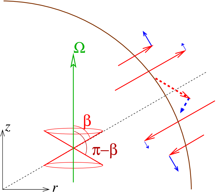
where $k=|\boldsymbol{k}|$. For free oscillations, presuming that the components of the wavevector $\boldsymbol{k}$ are at least approximately real (so that the envelope of the wave varies slowly with position), the dispersion relation requires that $-2\Omega\leq\omega\leq 2\Omega$. It is important that $\omega$ is independent of wavelength $\lambda=k/2\pi$; it depends only on the direction $\boldsymbol{\hat{k}}=\boldsymbol{k}/k$, which must lie on a double-napped cone whose axis is vertical, i.e. parallel to $\boldsymbol{\Omega}$, and whose half angle is

$$\beta\equiv\cos^{-1}\left|\frac{\omega}{2\Omega}\right|.$$ (10)

Hereafter, to fix important signs, we adopt the conventions $\omega\geq 0$ and $\Omega>0$. Tidal components that are retrograde with respect to the planetary spin will be represented by negative values of the azimuthal quantum number $m$ rather than negative values of $\omega$: that is, nonaxisymmetric tides have the $(\phi,t)$ dependence $\exp(im\phi-i\omega t)$ with $m\neq 0$, and their azimuthal pattern speed is $\omega/m$. With this convention, $\omega=|2\boldsymbol{\Omega}\boldsymbol{\cdot}\boldsymbol{k}|/k$, and the group velocity becomes

$$\boldsymbol{V}_{\rm gr}=\frac{\partial\omega}{\partial\boldsymbol{k}}=\mbox{sign}(k_{z})\frac{\boldsymbol{\hat{k}}\boldsymbol{\times}(2\boldsymbol{\Omega}\boldsymbol{\times}\boldsymbol{\hat{k}})}{k}.$$ (11)

So the waves and the energies they carry move crabwise, at right angles to their wavevectors.

The time-averaged energy density and energy flux carried by inertial waves are

$$\mathcal{E} = \frac{1}{4}\rho\boldsymbol{v}^{*}\boldsymbol{\cdot}\boldsymbol{v}=\frac{\rho k^{2}}{2(4\Omega^{2}-\omega^{2})}|\psi|^{2},$$ (12a)

$$\mathcal{F} = \mathcal{E}\boldsymbol{V}_{\rm gr},$$ (12b)

if the physical velocity perturbation is the real part of $\boldsymbol{v}$.

2.3 Tidal response of a coreless incompressible planet

Inasmuch as the planet is small compared to its orbital semimajor axis ($a$)—typically $R_{\rm p}/a\sim 10^{-2}$ for hot Jupiters—the dominant component of the external tidal potential is quadrupolar, that is, proportional to $R^{2}Y_{2,m}(\theta,\phi)\exp(-i\omega t)$ in spherical polar coordinates $R\theta\phi$ centered on the planet. Expressed in cartesians, $\Phi_{1,\rm ext}$ is then a linear superposition of the terms

$$m=\pm 2: A_{\pm 2}(x\pm iy)^{2}\,$$ (13a)

$$m=\pm 1: A_{\pm 1}z(x\pm iy)\,$$ (13b)

$$m=0: A_{0}(2z^{2}-x^{2}-y^{2}),$$ (13c)

times $\exp(-i\omega t)$, where the coefficients $A_{\pm 2}$, $A_{\pm 1}$ and $A_{0}$ are complex constants. On the other hand, it is clear that the wave equation (4) can be satisfied by polynomials in the cartesian coordinates. If the unperturbed body is axisymmetric—as it should be when $\Omega^{2}\ll\omega_{\rm dyn}^{2}$)—then after transients have died away, the forced responce of $\psi$ must have the same azimuthal symmetry as that of $\Phi_{1,\rm ext}$. If this response is also of second degree in the coordinates (an assumption that turns out to yield an acceptable solution), then its components at $m=\pm 1$ and at $m=\pm 2$ must have the same form as the first two of equations (13); it is easily seen that these satisfy the wave equation (2.1). But the axisymmetric component must have the form

$$m=0:\quad\psi \propto 2c^{2}z^{2}+x^{2}+y^{2}~{}+\mbox{constant},$$ (14)

which differs from that of the perturbing potential, eq. (13c).

Following eq. (3), the displacements associated with these quadratic forms of $\psi$ are linear functions of the coordinates. From this and the constancy of the density in the interior, it is easily shown that $\Phi_{1,\rm self}\propto\Phi_{1,\rm ext}$, so that the total potential perturbation $\Phi_{1}=\Phi_{1,\rm ext}+\Phi_{1,\rm self}$ is also a superposition of the terms (13), with an appropriate rescaling of the coefficients.

It remains to relate the amplitudes of $\psi$ and $\Phi_{1}$ using the surface boundary condition (5). If we neglect the influence of centrifugal force on the unperturbed state on the grounds that $\Omega^{2}\ll\omega_{\rm dyn}^{2}=4\pi G\rho$, the unperturbed boundary is spherical, $x^{2}+y^{2}+z^{2}=R_{\rm p}^{2}$, so that, with use of eq. (3),

$$\boldsymbol{v\cdot\hat{n}}=v_{R}=\frac{1}{i\omega R}\left[z\partial_{z}-c^{2}(x\partial_{x}+y\partial_{y})+\frac{2i\Omega c^{2}}{\omega}(y\partial_{x}-x\partial_{y})\right]\psi.$$ (15)

The solutions for the azimuthal harmonics of $\psi$ then turn out to be

$$\psi = \frac{3\omega(4\Omega^{2}-\omega^{2})}{8\pi G\rho(\omega-m\Omega)}\Phi_{1}\quad\mbox{if }m\in\pm 2,$$ (16a)

$$\psi = \frac{3\omega^{2}(4\Omega^{2}-\omega^{2})}{8\pi G\rho(\omega^{2}-2\Omega^{2}-m\Omega\omega)}\Phi_{1}\quad\mbox{if }m\in\pm 1,$$ (16b)

$$\psi = \frac{3(\omega^{2}-4\Omega^{2})}{8\pi G\rho}(x^{2}+y^{2}+2c^{2}z^{2})\frac{\Phi_{1}}{2R^{2}P_{2}(\cos\theta)}\quad\mbox{if }m=0.$$ (16c)

These have been calculated to lowest order in $\omega^{2}/\pi G\rho$ and $\Omega^{2}/\pi G\rho$, which are much less than unity. At this level of approximation, $\psi$ is negligible on the righthand side of the surface boundary condition (5), which therefore reduces to eq. (17), exactly as for the traditional equilibrium tide when rotation is neglected. Also to this order in $\Omega^{2}/\pi G\rho$, the boundary is spherical. A constant term in $\psi$ is not required even when $m=0$, since the radial velocity and radial displacement derived by substituting eq. (14) into eq. (15) turn out to be $\propto P_{2}(\cos\theta)$; this is no miracle, but rather a consequence of the fact that

$$\xi_{R}\approx-\frac{\Phi_{1}}{\bar{g}}\times[1+O(\Omega^{2}/\pi G\rho)]\,,$$ (17)

where $\bar{g}$ is the angular average of the surface gravity ($=4\pi G\rho R_{p}/3$ for a constant-density planet).

Inasmuch as $\omega$ and therefore $c$ are real, the responses (16) are perfectly in phase with the tidal forcing, so that there is no secular input of tidal energy to this (highly idealized) planet. An exception might occur if the denominator in eq. (16) were to vanish, when the tide would be in resonance with an $(\ell,m)=(2,1)$ free-precession mode. But this happens only at the single discrete frequency $\omega=\Omega$ [in inertial space, $\omega=2\Omega$], and then only if the spin and orbit are misaligned. So it cannot be a general explanation for tidal dissipation. Also, the responses (16) are entirely smooth and long-wavelength—or rather, nonwavelike, since the individual components of $\psi$ in (16) have no radial nodes at $R>0$, as is the case for $\Phi_{1}$ itself. Short-wavelength inertial oscillations are not excited. Note that the inner boundary condition (6) is satisfied because we are assuming that $R_{\rm c}=0$, and because all components of the velocities, being linear functions of the coordinates, vanish at the origin.

These results are hardly new. Solutions for the circular but not necessarily synchronized case are known as Roche-Riemann ellipsoids (Chandrasekhar, 1987). Viewed in the corotating frame of the orbit rather than that of the body’s spin, they appear as ellipsoids with stationary axes, though the flow velocity is generally nonzero in this frame. The axis ratios of these classical solutions are not limited to values near unity, as ours are; they are exact nonlinear solutions. Though exact, they are not always stable (Chandrasekhar, 1987). In fact Lebovitz & Lifschitz (1996) have shown that except for the synchronous solutions, the Riemann and Roche-Riemann ellipsoids are generically vulnerable to small-scale parametric instabilities, with growth rates that increase with increasing departure from stationary and circular streamlines. However, the growth of small-scale inertial waves by parametric instability is entirely distinct from direct tidal forcing, and the secular energy dissipation rate that results is much more difficult to estimate because it depends upon the amplitudes at which these instabilities saturate, which necessarily involves nonlinear considerations (Arras et al., 2003, and references therein).

We conjecture that the absence of small-scale waves from the tidal response is not a peculiarity of the incompressible, constant-density limit, but that it holds more generally for isentropic, coreless, compressible bodies whose unperturbed enthalpy profiles are sufficiently smooth, provided that the outer boundary is free. This conjecture, if true, would seem to contradict the results of Wu (2005b). More will be said on this subject in §4.1.

3 Production of short waves by scattering from the core

When the radius of the rigid core is nonzero, it does not seem to be possible to construct a purely nonwavelike tidal response, confirming what OL04 concluded from numerical computations with a compressible model. As far as we can tell, this remains true even in our incompressible, constant-density model, at least in the limit that the tide is strictly periodic. It seems that it ought to be possible to prove (or disprove) this rigorously. We have no such proof, but we explain briefly why we think it is true in §3.1; the material of that subsection is not used in the rest of the paper. Then in §3.2, we go on to the main goal of this section, which is to estimate the production of short waves at the core on the assumption that the response is partly wavelike.

3.1 Homogeneous solutions of the wave equation

The difficulty in constructing a purely nonwavelike response appears to lie in the lack of a sufficiently rich set of homogenous functions that solve equation (4) and are nonsingular on the surface of a sphere, or indeed any closed surface. A function $f(x,y,z)$ is said to be homogenous of degree $D$ if $f(\sigma x,\sigma y,\sigma z)=\sigma^{D}f(x,y,z)$ for any constant $\sigma\neq 0$; the degree may be negative. A homogeneous function cannot have isolated radial nodes, since if it vanishes at any point, then it must vanish at all points along the same radial ray. But of course a linear combination of such functions may have radial nodes.

If $c^{2}<0$, as when $\omega^{2}>4\Omega^{2}$ [cf. eq. (8], then equation (4) is elliptic rather than hyperbolic, and after the rescaling $z=z/\sqrt{-c^{2}}$, reduces to Laplace’s equation. Solid spherical harmonics $r^{\ell}Y_{\ell,m}(\theta,\phi)$, when expressed in cartesians, are homogeneous solutions—in fact polynomials—of degree $D=\ell\geq 0$. Each of these functions has a companion $r^{-\ell-1}Y_{\ell,m}(\theta,\phi)$ with negative degree, $D=-(\ell+1)$, that also solves Laplace’s equation. Given smooth values of $\psi$ or $\partial\psi/\partial n$ on concentric spheres or (less conveniently) on spheroids, it is possible to construct a smooth solution of Laplace’s equation in the space between them as linear combination of these functions; in general, unless the boundary conditions are very restricted, both signs of $D$ are required.

As is well known, the spherical harmonics of a given degree $\ell$ constitute an irreducible representation of the rotation group $SO(3)$, to which the laplacian is invariant. This suggests that when $\omega^{2}<4\Omega^{2}$, we should be concerned with homogeneous functions that belong to irreducible representations of $SO(2,1)$, the 2+1-dimensional version of the Lorentz group, since that is the group under which the d’Alembertian operator in eq. (4) is invariant when $c^{2}>0$. Let $s^{2}\equiv x^{2}+y^{2}-(cz)^{2}$ and let $\eta\in(-\infty,\infty)$ be a real-valued hyperbolic angle, and let $\phi\in(-\pi,\pi]$ be the usual azimuthal angle. Then the following parametrizations cover the “future,” “past” and “absolute elsewhere” of the origin, respectively:

$$(x,y,cz) =(|s|\cos\phi\sinh\eta,\,|s|\sin\phi\sinh\eta,\,|s|\cosh\eta) s^{2} <0,~{}z>0;$$

$$(x,y,cz) =(|s|\cos\phi\sinh\eta,\,|s|\sin\phi\sinh\eta,\,-|s|\cosh\eta) s^{2} <0,~{}z<0;$$

$$(x,y,cz) =(|s|\cos\phi\cosh\eta,\,|s|\sin\phi\cosh\eta,\,|s|\sinh\eta) s^{2} >0\,.$$

Suitable homogeneous polynomials that satisfy eq. (4) in these three regions and belong to irreducible representations of $SO(2,1)$ are

$$(-s^{2})^{\ell/2}i^{m}Y_{\ell,m}(i\eta,\phi)\quad(-s^{2})^{\ell/2}i^{m}Y_{\ell,m}(\pi-i\eta,\phi),\quad\mbox{and}\quad(s^{2})^{\ell/2}i^{m}Y_{\ell,m}({\textstyle\frac{\pi}{2}}-i\eta,\phi).$$ (18)

The tidal response of a coreless incompressible planet is made up of linear superpositions of these: for example, eq. (16c) is proportional to $s^{2}Y_{2,0}(i\eta,\phi)$ in the “future.” In order to accommodate the boundary condition $v_{R}=0$ at the surface of a finite core, one would like to add to the polynomial solutions (16) a suitable linear combination of homogenous solutions of negative degree. The negative-degree solutions would be larger near the core than near the surface, and therefore could “patch up” the boundary condition at the core without much spoiling the boundary condition at the surface. The obvious negative-degree counterpart to the first of the functions eq. (18), by analogy with the case of Laplace’s equation, is $(-s^{2})^{-(\ell+1)/2}i^{m}Y_{\ell,m}(i\eta,\phi)$. While this is indeed a solution of the wave equation, it is unfortunately singular where the core intersects the “light cone” $s^{2}=0$, i.e. at the critical colatitudes $\theta=\beta$ and $\theta=\pi-\beta$ [eq. (10)]. So it seems that we cannot superpose a finite number of finite-degree homogeneous solutions to construct a smooth response.

3.2 WKB scattering calculation

3.2.1 Nonspecular reflection from a planar boundary

To see how short inertial waves may be produced from long ones, consider the reflection of an incident plane wave,

$$\psi_{\rm in}(\boldsymbol{x},t)=A_{\rm in}e^{i\boldsymbol{k}\boldsymbol{\cdot}\boldsymbol{x}-i\omega t}\,,$$

from a planar wall with normal $\boldsymbol{\hat{n}}$ pointing away from the fluid. The reflection is generally not specular, and the incident and scattered wavelengths differ, unless $\boldsymbol{\hat{n}}$ is parallel or perpendicular to $\boldsymbol{\Omega}$. These are consequences of the anisotropy of the dispersion relation (9) and would also hold, with some quantitative changes, were buoyancy important.

If the wall is fixed in the unperturbed frame of the fluid and sufficiently rigid so that any transmitted wave is negligible, then energy conservation requires a reflected wave. This is enforced by the boundary condition, which we have taken to be $\boldsymbol{\hat{n}}\boldsymbol{\cdot}\boldsymbol{v}=0$, but any other non-absorbing boundary condition would lead to the same relationship between the incident and reflected wavevectors as the one we are about to derive.

The scattered (outgoing) wavevector $\boldsymbol{k}^{\prime}$ is determined by two conditions. First, in order that the incident and scattered wave have the same relative phase at all points along the wall, as required by the boundary condition that connects them, it is necessary that $\boldsymbol{k}$ and $\boldsymbol{k}^{\prime}$ have the same components parallel to the wall: that is, $\boldsymbol{\hat{n}}\boldsymbol{\times}(\boldsymbol{k}^{\prime}-\boldsymbol{k})=0$, or equivalently

$$\boldsymbol{k}^{\prime}=k^{\prime}_{\perp}\boldsymbol{\hat{n}}+(\boldsymbol{k}-\boldsymbol{\hat{n}}\boldsymbol{\hat{n}}\boldsymbol{\cdot}\boldsymbol{k})\equiv k^{\prime}_{\perp}\boldsymbol{\hat{n}}+\boldsymbol{k}_{\parallel}\,,$$ (19)

where $k^{\prime}_{\perp}$ remains to be determined. Similarly, in order that the relative phase be constant in time, the two waves must have the same frequency, $\omega$. Substituting from eq. (19) for $\boldsymbol{k}^{\prime}$ into $(k^{\prime})^{2}\omega^{2}=(2\boldsymbol{\Omega}\boldsymbol{\cdot}\boldsymbol{k}^{\prime})^{2}$ leads to

$$\left[(2\boldsymbol{\Omega}\boldsymbol{\cdot}\boldsymbol{\hat{n}})^{2}-\omega^{2}\right](k^{\prime}_{\perp})^{2}+8(\boldsymbol{\Omega}\boldsymbol{\cdot}\boldsymbol{k}_{\parallel})(\boldsymbol{\Omega}\boldsymbol{\cdot}\boldsymbol{\hat{n}})k^{\prime}_{\perp}+(2\boldsymbol{\Omega}\boldsymbol{\cdot}\boldsymbol{k}_{\parallel})^{2}-\omega^{2}k_{\parallel}^{2}=0.$$ (20)

It is clear that one of the roots of this quadratic equation must be the known solution $k^{\prime}_{\perp}=k_{\perp}$ representing the incident wave, and therefore the product of the distinct roots is

$$k_{\perp}k^{\prime}_{\perp}=\frac{\omega^{2}\boldsymbol{k}_{\parallel}^{2}-(2\boldsymbol{\Omega}\boldsymbol{\cdot}\boldsymbol{k}_{\parallel})^{2}}{\omega^{2}-(2\boldsymbol{\Omega}\boldsymbol{\cdot}\boldsymbol{\hat{n}})^{2}}\,.$$ (21)

The denominator in eq. (21) may vanish when the numerator does not: the reflected wavevector then becomes infinite and normal to the boundary. We believe that the change of wavelength upon reflection, which is a direct consequence of the inertial-wave dispersion relation, underlies the singular behavior observed by OL04 in their numerical calculations.

Figure 1: Scattering of a long wave into a short one at the core near the northern critical latitude. Allowed directions for $\boldsymbol{k}$ make angles $\beta$ or $\pi-\beta$ with $\boldsymbol{\Omega}$, as shown by “light cone.” Large diagonal solid arrows (red in online version) are outgoing $\boldsymbol{k}_{\rm out}$. These become infinite and change sign across critical latitude (thin dashed line). Smaller solid arrows (blue online) show group velocity $\boldsymbol{V}_{\rm g,out}$, whose magnitudes are $\propto k^{-1}$. Heavy dashed arrows show the incoming $\boldsymbol{k}_{\rm in}$ and its associated group velocity. These are not to scale: $k_{\rm in}\ll k_{\rm out}$ and $V_{\rm g,in}\gg V_{\rm g,out}$. In fact, all of the red arrows should have latitudinal components that are nearly the same in magnitude and sign, $\approx k_{\theta,\rm in}>0$.

3.2.2 Scattering from a spherical core

Now we apply this idea to scattering of the “equilibrium tide” from the spherical core. As noted in §2.3, the equilibrium tide is radially nodeless, and in this sense nonwavelike. However, the functions (16) do have nodes in angular directions: the wavenumber parallel to the surface of the core of these quadratic functions is roughly

$$\boldsymbol{k}_{\parallel}\approx\pm\frac{2}{R_{\rm c}}\boldsymbol{\hat{e}}_{\theta}\pm\frac{m}{R_{\rm c}\sin\theta}\boldsymbol{\hat{e}}_{\phi}\equiv k_{\theta}\boldsymbol{\hat{e}}_{\theta}+k_{\phi}\boldsymbol{\hat{e}}_{\phi}$$ (22)

at colatitude $\theta$. Since $|k_{\parallel}R_{\rm c}|>1$, we may expect that WKB should be applicable to an outgoing wave whose radial wavenumber $k^{\prime}_{\perp}$ is real and $\gg 1/R_{\rm c}$. We cannot make use of eq. (21) because the incident component $k_{\perp}$ is ill-defined and the equilibrium tide does not satisfy the WKB dispersion relation. But equation (20) should still be applicable to the short-wavelength outgoing wave. It can be seen that the coefficient of $k^{\prime}_{\perp}$ vanishes at the critical latitudes $\theta=\beta$ and $\theta=\pi-\beta$, where $\beta$ is defined by eq. (10).

The large root of eq. (20) can be found by balancing the terms in $k^{\prime}_{\perp}$ and $(k^{\prime}_{\perp})^{2}$:

$$k^{\prime}_{R} \approx \frac{8(\boldsymbol{\Omega}\boldsymbol{\cdot}\boldsymbol{k}_{\parallel})(\boldsymbol{\Omega}\boldsymbol{\cdot}\boldsymbol{\hat{n}})}{\omega^{2}-(2\boldsymbol{\Omega}\boldsymbol{\cdot}\boldsymbol{\hat{n}})^{2}}=\frac{k_{\theta}\sin 2\theta}{\cos^{2}\theta-\cos^{2}\beta}$$ (23)

$$\approx \begin{cases}k_{\theta}\csc(\beta-\theta)&\mbox{near}~{}\theta=\beta\\ k_{\theta}\csc(\beta+\theta)&\mbox{near}~{}\theta=\pi-\beta.\end{cases}$$

Let us now determine when the large root represents an outgoing wave. Since $|k^{\prime}_{R}|\gg k_{\parallel}$, we may write $\boldsymbol{\hat{k}}^{\prime}\approx\mbox{sign}(k^{\prime}_{R})\boldsymbol{\hat{e}}_{R}+|k^{\prime}_{R}|^{-1}\boldsymbol{k}_{\parallel}$ through first order in $k_{\parallel}/k^{\prime}_{R}$, whence from eq. (11),

$$\boldsymbol{V}_{\rm gr}\approx 2\Omega\sin\beta\,\mbox{sign}(\cos\theta)\left(\frac{k_{\theta}}{(k^{\prime}_{R})^{2}}\boldsymbol{\hat{e}}_{R}-\frac{1}{k^{\prime}_{R}}\boldsymbol{\hat{e}}_{\theta}\right)$$ (24)

near the critical latitudes. The radial component of this is positive when $\mbox{sign}(k_{\theta})=\mbox{sign}(\cos\theta)$, so this becomes the condition for the outgoing wave: $k_{\theta}>0$ at the northern critical latitude, and $k_{\theta}<0$ at the southern one. Also, it can be seen from eqs. (24) & (23) that the group velocity is predominantly latitudinal and directed away from the critical latitude: that is, towards the pole on the poleward side, and toward the equator on the equatorial side.

Next, we determine the amplitude of the outgoing wave by matching it to the positive-$k_{\theta}$ component of the incident wave via the boundary condition $\boldsymbol{\hat{e}}_{R}\boldsymbol{\cdot}(\boldsymbol{v}_{\rm in}+\boldsymbol{v}_{\rm out})=0$. The radial velocity $v_{R}$ is related to $\psi$ by eq. (15) in cartesians, and in spherical polars [cf. eq. (3)]

$$v_{R}=\frac{1}{i\omega\sin^{2}\beta}\left[(\cos^{2}\theta-\cos^{2}\beta)\frac{\partial\psi}{\partial R}-\frac{\sin 2\theta}{2R}\frac{\partial\psi}{\partial\theta}+\frac{m\cos\beta}{R}\psi\right].$$ (25)

For the outgoing wave, this reduces at the critical latitudes to

$$v_{R,\rm out}\approx\frac{|k_{\theta}|R_{\rm c}\sin\beta-im}{2\Omega R_{\rm c}\sin^{2}\beta}\psi_{\rm out}\,.$$

The contribution from $\partial_{R}\psi$ is finite and $\propto k_{\theta}$ despite the fact that $k^{\prime}_{R}$ diverges, because of the factor $(\cos^{2}\theta-\cos^{2}\beta)$ in front of $\partial\psi_{\rm out}/\partial R$. For the “incoming” equilibrium tide, the expression is similar, except that $\partial_{R}\psi_{\rm in}$ doesn’t contribute because $\partial\psi_{\rm in}/\partial R$ is finite at the critical latitude:

$$v_{R,\rm in}\approx\frac{-|k_{\theta}|R_{\rm c}\sin\beta-im}{2\Omega R_{\rm c}\sin^{2}\beta}\psi_{\rm in}\,.$$

Combining the last two equations, we have the following relation between the long-wavelength “ingoing” tide and the short-wavelength outgoing wave:

$$A_{\rm out}\approx\frac{|k_{\theta}|R_{\rm c}\sin\beta-im}{|k_{\theta}|R_{\rm c}\sin\beta+im}A_{\rm in}\,.$$ (26)

Thus, the boundary condition $\xi_{R,\rm out}=-\xi_{R,\rm in}$ at the core leads to $|A_{\rm out}|=|A_{\rm in}|$.

The relationship between the amplitude $A_{\rm in}$ of the “incident” component of the equilibrium tide and the tidal potential $\Phi_{1}$ is given by equations (16). For definiteness, consider a synchronization tide exerted on a planet in a circular orbit, so that

$$m=2\mbox{\,sign}(n-\Omega),\ \mbox{and}\ \omega=2|n-\Omega|,\ \mbox{where}\ n\equiv\frac{2\pi}{P_{\rm orb}}$$ (27)

is the mean motion. In this case, the relevant component of $\Phi_{1}$ becomes

$$\Phi_{1}\to-\frac{3fGM_{*}}{4a^{3}}R^{2}\sin^{2}\theta e^{im\phi-i\omega t}\,.$$ (28)

The factor $f$ represents the ratio $\Phi_{1}/\Phi_{1,\rm ext}$ of the total perturbing potential to that part which is exerted by the companion. In general, $f\approx 1+2k_{\rm p}$ at the surface, $R=R_{p}$, where $k_{\rm p}$ is the apsidal-motion constant, equal to one half the planetary Love number. For a constant-density coreless planet, $f=5/2$. Expanding $\sin^{2}\theta$ and extracting the coefficient of $\exp(2i\theta)$ leads to

$$\quad A_{\rm in}=-\frac{9f}{16}\frac{\omega(\omega+m\Omega)}{8\pi G\rho}\frac{GM_{*}R_{c}^{2}}{a^{3}}\quad\mbox{for $|m|=2$ and $e=0$}.$$ (29)

3.2.3 Energy flux and power of the scattered waves

Since $|\psi_{\rm out}|=|A_{\rm in}|$ equations (12), (24), and (29) imply that the radial component of the energy flux in the outgoing short waves at the core is

$$\mathcal{F}_{R}=\frac{\rho|A_{\rm in}|^{2}}{R_{\rm c}\sqrt{4\Omega^{2}-\omega^{2}}}\approx\left(\frac{3fM_{*}R_{\rm p}^{3}}{32M_{\rm p}a^{3}}\right)^{2}\frac{\omega^{2}(\omega+m\Omega)^{2}}{\sqrt{4\Omega^{2}-\omega^{2}}}\rho R_{\rm c}^{3}$$ (30)

for the $|m|=2$ synchronization tide, i.e. for the tidal response of a planet in a circular orbit with aligned but nonsynchronous rotation. Expressions for $\omega$ and $m$ in terms of the orbital and rotational periods were given above in §3.2.2. As it stands, eq. (30) is valid only for a constant-density planet (so that $f=5/2$), and only for the waves launched sufficiently close to the critical latitude so that we may take $|\boldsymbol{k}^{\prime}|\approx|k^{\prime}_{R}|\gg k_{\theta},\,k_{\phi}$. We have taken $|k_{\theta}|\approx 2/R_{\rm c}$ and $k_{\phi}=m/R$, as appropriate for the response (16) to an $|m|=\ell=2$ tidal potential. Notice that the large radial wavenumber has canceled between the wave energy density (12a) and radial group velocity (24), so that the flux is approximately independent of latitude, provided that $\theta$ is sufficiently close to $\beta=\cos^{-1}(\omega/2\Omega)$ or to $\pi-\beta$. Let us therefore integrate over latitudinal bands of width $2\Delta\theta$ centered on both critical latitudes, with $\Delta\theta\ll\beta,\pi-\beta$, to obtain the total mechanical power carried radially outward by the short waves launched within these bands:

$$\dot{E}(\Delta\theta) \approx 8\pi R_{\rm c}^{2}\sin\beta\Delta\theta\times\mathcal{F}_{R}$$ (31)

$$\approx 2\pi\left(\frac{3f}{16}\right)^{2}\omega(\omega+m\Omega)^{2}\left(\frac{M_{*}R_{\rm p}^{3}}{M_{\rm p}a^{3}}\right)^{2}\rho R_{\rm c}^{5}\Delta\theta.$$

Although eq. (31) has been derived for an incompressible, constant-density planet, it can be generalized to an isentropic compressible body with standard approximations for the equilibrium tide. In our approach where the core is regarded as a perturbation to an otherwise homogeneous body, we continue to calculate the equilibrium tide as if the core were absent. What is needed for the scattering calculation is the radial displacement of the equilibrium tide at the core, $\xi_{R}^{\rm eq}(R_{\rm c})$ For a constant-density body, the radial strain $\sigma\equiv\xi_{R}(R)/R$ is independent of radius $R$, so

$$\xi^{\rm eq}_{R}(R_{\rm c})=\frac{R_{\rm c}}{R_{\rm p}}\xi^{\rm eq}_{R}(R_{\rm p})\approx-\frac{R_{\rm c}}{R_{\rm p}}\frac{\Phi_{1}(R_{\rm p})}{g_{\rm p}}=-f\left(\frac{R_{\rm p}}{a}\right)^{3}\frac{M_{*}}{M_{\rm p}}R_{\rm c},$$ (32)

where $a$ is the semimajor axis of the orbit, $g_{\rm p}=GM_{\rm p}/R_{\rm p}^{2}$, and the surface displacment has been evaluated from (5) with neglect of $\psi$ on the righthand side as before, i.e. $\xi_{R}(R_{\rm p})\approx-\Phi_{1}(R_{\rm p})/g_{\rm p}$. We assume that the relation (32) between the surface displacement of the equilibrium tide and the disturbing potential holds in general, provided that $f$ is interpreted as $1+2k_{\rm p}$ for the relevant value of the apsidal motion constant $k_{\rm p}$. The latter is $k_{\rm p}\approx 0.260$ for an $n=1$ Emden polytrope, which roughly approximates a Jovian planet, as compared to $k_{\rm p}=3/4$ for a constant-density body ($n=0$ polytrope). However, since the radial strain of the tide is not constant with radius in general, we must multiply $f$ in eq. (32) by a factor $\sigma(R_{\rm c})/\sigma(R_{\rm p})$ to obtain the correct displacement at the core. If the core is sufficiently small, $R_{\rm c}\lesssim R_{\rm p}/2$, then $\sigma(R_{\rm c})\approx\sigma(0)$.

It is not immediately clear how to estimate $\sigma(0)$ easily. One possibility is to assume that $\xi_{R}^{\rm eq}$, which represents the radial displacement of the fluid by the equilibrium tide, is the same as the radial displacement of the equipotential surfaces between the undistorted and distorted states; then it can be shown by integration of the Radau equation from which $k_{\rm p}$ is obtained (Schwarzschild, 1958) that $\sigma(0)/\sigma(R_{\rm p})\approx(1+2k_{\rm p})^{-1}\approx 0.658$ for the $N=1$ polytrope, so that the factor in square brackets in (32) reduces to unity for $N=1$. Alternatively, if one evaluates $\xi_{R}^{\rm eq}$ from the summed zero-frequency response of all the normal modes, taking into account their overlap with the quadrupolar perturbing potential $\Phi_{1,\rm ext}$, then it can be shown that $\sigma(0)/\sigma(R_{\rm p})\approx 0.813$ at $N=1$. By far the largest response is that of the $\ell=2$ fundamental mode, for which $\xi_{R}$ is nearly linear in $R$. These two estimates of $\sigma(0)/\sigma(R_{\rm p})$ differ because, even for an originally spherical and nonrotating body, the radial displacements of the fluid and of the equipotentials need not coincide except at the surface. There are many possible displacement fields that can be compatible with a given distortion of the density and potential fields, and it is not possible to choose among them on the basis of the continuity equation alone without some auxiliary constraint. It can be shown that in a stratified region, the appropriate constraint is $\boldsymbol{\nabla\cdot\xi}=0$ even for a compressible body: the density and pressure of fluid elements is not disturbed by the equilibrium tide in the stratified case. OL04 adopted this constraint. For an isentropic region in a nonrotating star, the appropriate constraint is $\boldsymbol{\nabla\times\xi}=0$ rather than $\boldsymbol{\nabla\cdot\xi}=0$ since vorticity is conserved; in a compressible body, this leads to a different pattern of fluid displacements for the same distortion of the density and potential (Goodman & Dickson, 1998; Terquem et al., 1998). Thus our second estimate (the one yielding $0.813$) was calculated under the assumption that $\boldsymbol{\xi}=\boldsymbol{\nabla}\chi$ for some scalar function $\chi$. Since our bodies rotate, however, the axial component of vorticity does not vanish and therefore $\boldsymbol{\nabla\times\xi}=0$ may not be the correct constraint. For the purpose of estimating the order of magnitude of the tidal $Q$ that results from scattering by the core, the differences among $0.658$, $0.813$, and unity (the correct result for $N=0$) are not important, and we take this as an indication that the true value of $\sigma(0)/\sigma(R_{\rm p})$ is also sufficiently close to unity.

The frequency-dependent factor $\omega(\omega+m\Omega)$ in eq. (31) becomes $8|n-\Omega|n^{2}$ with use of (27). Finally, the relevant density is the density of the fluid at the surface of the core, $\rho(R_{\rm c})$. With these modifications, the wave power (31) generalizes to

$$\dot{E}(\Delta\theta)\approx|n-\Omega|n^{2}\frac{9\pi}{16}\left[(1+2k_{\rm p})\frac{\sigma(R_{\rm c})}{\sigma(R_{\rm p})}\right]^{2}\left(\frac{M_{*}}{M_{\rm p}}\right)^{2}\left(\frac{R_{\rm p}}{a}\right)^{6}\rho(R_{\rm c})R_{\rm c}^{5}\Delta\theta.$$ (33)

The tidal torque, or more precisely, the rate of increase of the angular momentum carried by the waves, is $\Gamma=\dot{E}\times m/\omega=\dot{E}/(n-\Omega)$. Thus according to eq. (33), the torque has the same sign as $n-\Omega$—meaning that subsynchronous planets spin up and supersynchronous ones spin down—but is independent of the magnitude of the departure from synchronous rotation. This is probably not true if the departure is very small, $|n-\Omega|\ll n$: in that limit, the critical latitudes converge upon the equator from both sides, whereas the approximations used to derive eq. (33) implicitly assume that these latitudes are well separated from one another.

3.2.4 Dissipation of the short waves, and the tidal $Q$

Waves that do not dissipate appreciably before returning to the region from which they are launched (perhaps after multiple reflections between the outer boundary and the core, with changes of wavelength at each reflection) must be treated as global normal modes. Secular input of energy and angular momentum to nondissipative global modes would occur only at exact resonance with the tide, which would almost never occur for modes of finite wavelength. Furthermore, the angular momentum carried by the waves is not transferred to the mean flow, and therefore does not alter the angular velocity $\Omega$, until those waves dissipate.

Thus, in order to estimate $Q$, we must consider the dissipation of the waves. Unfortunately, this is a complicated issue. More than one process may be important, depending upon aspects of the planetary structure and transport processes that can justifiably be neglected in calculating the wave excitation. Nevertheless, some dissipative processes can be ruled out, and a rough upper limit on $Q$ as a function of the core radius can be obtained.

First of all, the narrower the width $\Delta\theta$ of the latitudinal bands around critical latitudes that we consider, the shorter is the wavelength of the waves launched within those bands: eq. (23) shows that $\lambda\sim\pi R_{\rm c}\Delta\theta$. All of the obvious dissipation mechanisms become more efficient as wavelength decreases. The rate of viscous dissipation, for example, scales as $\nu k^{2}$, and therefore $\propto|\Delta\theta|^{-2}$. Furthermore, the propagation time from the core to the surface of the planet—or rather, to the upper boundary of the convection zone, since in a realistic hot Jupiter there must be a stratified region near the surface—scales $\propto\lambda\propto\Delta\theta$. [Eq. (24) says that the radial component of the group velocity starts out at $V_{{\rm gr},R}\sim\Omega\lambda^{2}/R_{\rm c}$. But this is because the rays emanating from near the critical latitude are almost tangential to the core. The rays follow straight lines in the meridional plane, and $\lambda$ is approximately constant along them, so that a more representative value of the group velocity for the purpose of estimating the propagation time is $|\boldsymbol{V}_{\rm gr}|\sim\Omega\lambda\sim\Omega R_{\rm c}\Delta\theta$.] Hence the number of viscous dissipation times per transit time scales $\propto|\Delta\theta|^{-3}$.

Nevertheless viscous dissipation is probably negligible, as can be seen by very rough order of magnitude considerations. Goldreich & Nicholson (1977) estimated that turbulent convective viscosity acting on the equilibrium tide, which has a “wavelength” $\sim R_{\rm p}$, would yield $Q\approx 10^{13}$ because of suppression of turbulent viscosity by a factor $(\omega\tau_{\rm c})^{-2}$, where $\tau_{\rm c}$ is the turnover time of the largest eddies. (When this argument applies, the $Q$ based on the laminar viscosity should be even larger.) In our case, the suppression factor would not be quite so small because the tidal period is a few days even for a substantially nonsynchronous rotation, rather than 5 hours as for the Jupiter-Io system. So by Goldreich and Nicholson’s reasoning, $Q\sim 10^{11}$ for the equilibrium tide in our case. The short waves have the same period as the tide itself, so the suppression factor is the same for them, but their damping rate is increased by a factor $\sim(kR)^{2}\sim|\Delta\theta|^{-2}$, and allowing for their transit time between the core and the surface, we may conclude that the $Q$ value due to turbulent convective damping of short waves should be at least $10^{11}|\Delta\theta|^{3}$ in hot Jupiters. We have stated this as an inequality because the core is small and therefore somewhat inefficient at scattering the equilibrium tide; this will be made more quantitative below, but for now, note simply that the wave power (33) is $\propto R_{\rm c}^{5}$. To be astrophysically relevant, $Q$ should be of order $10^{5}$ to $10^{6}$. Therefore only waves within $\Delta\theta\lesssim 10^{-2}$ radians of the critical latitude could damp effectively by this mechanism. But as we will soon show, other mechanisms exist that can damp the waves launched farther from the critical latitude, and since the wave power $(\ref{eq:power})$ is proportional to $\Delta\theta$, these mechanisms give a smaller $Q$.

An important source of dissipation for short inertial waves in hot Jupiters is escape from the convection zone, where most of the mass of the planet resides, into the stratified radiative zone near the surface, whose existence is guaranteed by strong illumination from the host star. In the radiative zone the waves convert into g modes (more properly, Hough modes) that are supported primarily by buoyancy rather than Coriolis forces. They are then subject to damping by radiative diffusion because they perturb the temperature and entropy profiles. Radiative diffusion damps more efficiently than viscosity because of the much longer mean free path of photons compared to molecules or ions, and it is all the more efficient because the wavelength in the radiative zone shortens by a further factor $\sim\Omega/N\sim 10^{-2}$, where $N$ is the Brunt-Väsälä frequency there. The upshot is that an outgoing short inertial wave that penetrates the radiative zone will almost certainly damp before returning to the core. Details will be given by Eric Johnson in a forthcoming paper. Here we simply note that penetration is not possible between the poles and the critical latitudes, because the Hough modes are evanescent there. Using the fact that the group velocities lie at angles $(\pi/2)\pm\beta$ with respect to the polar axis in the meridional plane, one can show with a little trigonometry that penetration into the radiative zone can occur at the first encounter only if

$$\frac{R_{\rm c}}{R_{\rm s}}\cos\Delta\theta < \frac{\omega^{2}}{2\Omega^{2}}-1\quad\mbox{(poleward rays)}$$

$$\frac{R_{\rm c}}{R_{\rm s}}\cos\Delta\theta > 1-\frac{\omega^{2}}{2\Omega^{2}}\quad\mbox{(equatorward rays)},$$ (34)

where $R_{\rm s}\approx R_{\rm p}>R_{\rm c}$ is the radius at the convective-radiative interface. A poleward ray is one that is launched between the critical latitude and the pole, so that it starts out toward the rotation axis, etc. Neither inequality in (3.2.4) can be satisfied when $\omega<\Omega\sqrt{2}$, i.e. $\beta>\pi/4$. In such cases the waves are fully reflected at their first encounter with the radiative zone and return toward the core. But the ray may enter the radiative zone on a subsequent encounter.

Paradoxically, the easiest damping mechanisms to predict with confidence by analytic means may be the nonlinear ones. It is reasonable to assume that any inertial wave whose velocity amplitude satisfies $v\gtrsim\omega/k$ will quickly damp by some combination of Kelvin-Helmholtz instabilities or three-mode coupling to even shorter-wavelength daughter modes, as is observed for closely related internal waves (g-modes), both in the laboratory and in the oceans (e.g. McEwan, 1971; Müller et al., 1986). This process is effectively local, occuring on lengthscales comparable to the wavelength and timescales comparable to the wave period. The dimensionless nonlinearity parameter $kv/\omega$ diverges rapidly toward the critical latitude. From eqs. (12), $|\boldsymbol{v}|^{2}=4\mathcal{F}_{R}/\rho V_{{\rm g},R}$; substituting then from eqs. (24) and (30), and generalizing the latter in the same way that we turned eq. (31) into eq. (33), we find that

$$\frac{kv}{\omega}\approx\left[\frac{3}{2\sqrt{8}}(1+2k_{\rm p})\frac{\sigma(R_{\rm c})}{\sigma(R_{\rm p})}\,\sqrt{\frac{\omega+m\Omega}{\omega-m\Omega}}\right]\frac{M_{*}R_{\rm p}^{3}}{M_{\rm p}a^{3}}\,(\Delta\theta)^{-2}\,.$$ (35)

The contents of the square brackets above are close to unity. Therefore, nonlinear dissipation will dominate within latitudinal bands of halfwidth

$$\Delta\theta_{\rm nl}\approx\left(\frac{M_{*}R_{\rm p}^{3}}{M_{\rm p}a^{3}}\right)^{1/2}\approx 0.03\left(\frac{R_{\rm p}}{R_{\rm J}}\right)^{3/2}\left(\frac{M_{\rm p}}{M_{\rm J}}\right)^{1/2}\left(\frac{4\,{\rm d}}{P}\right)\,\mbox{radians.}$$ (36)

Though small compared to unity, this is indeed larger than the generous estimate made above for the latitudinal distance within which turbulent convective viscosity might be important. We regard this as a lower bound on the value of $\Delta\theta$ within which the waves are able to dissipate, since other mechanisms—especially escape into the radiative zone—may contribute.

The tidal $Q\equiv\omega\Delta E/\dot{E}$, where $\Delta E$ is the maximum potential energy associated with the time-variable part of the tidal distortion. The instantaneous gravitational energy of the equilibrium response to an applied quadrupole $\Phi_{1,\rm ext}(R,\theta,\phi)=KR^{2}P_{2}(\cos\gamma)$ is $k_{\rm p}K^{2}R_{\rm p}^{5}/G$; here $K$ is a constant and $\gamma$ is the angle between the symmetry axis of the potential and the point $\boldsymbol{R}$. For the present case of a synchronization tide, $K=-\sqrt{3/2}GM_{*}/a^{3}$ [eq. (A1)], so

$$\Delta E=\frac{3}{2}k_{\rm p}\frac{GM_{*}^{2}R_{\rm p}^{5}}{a^{6}}\,.$$ (37)

Using eq. (27) & (33) and taking $k_{\rm p}\approx 0.26$ and $\rho(R_{\rm c})\approx(\pi M_{\rm p}/4R_{\rm p}^{3})$ as appropriate for the apsidal motion constant and central density of a homogeneous $N=1$ polytrope, we have

$$Q \approx \frac{16k_{\rm p}}{3\pi^{4}}\left[(1+2k_{\rm p})\frac{\sigma(R_{\rm c})}{\sigma(R_{\rm p})}\right]^{-2}P^{2}\frac{GM_{\rm p}R_{\rm p}^{2}}{R_{\rm c}^{5}}(\Delta\theta)^{-1}$$ (38)

$$\approx 2.1\times 10^{7}\left(\frac{P}{4\,{\rm d}}\right)^{2}\left(\frac{M_{\rm p}}{M_{\rm J}}\right)\left(\frac{R_{\rm p}}{R_{\rm J}}\right)^{2}\left(\frac{R_{\rm c}}{0.2R_{\rm J}}\right)^{-5}\left(\frac{\Delta\theta}{0.1\,{\rm rad}}\right)^{-1}.$$

In the final line, we have taken the square brackets equal to unity. This result is some two orders of magnitude larger than is typically assumed for hot Jupiters but is obviously very sensitive to the assumed core radius. The fiducial value $R_{\rm c}\approx 0.2R_{\rm J}$ is a crude estimate based on the assumptions that $M_{\rm c}\approx 0.1M_{\rm p}$ and that the core must be roughly twice as dense as its immediate surroundings at the same pressure because it has roughly twice the molecular weight per electron. Here $P$ is the period of the orbit ($P=2\pi/n$), not the period of the tide ($P_{\rm tide}=\pi/|n-\Omega|$): $Q$ turns out to be independent of the latter. The $Q$ for circularization of a slightly eccentric but synchronous orbit is nearly the same for this mechanism if the same $\Delta\theta$ applies (see the Appendix).

Values for $Q$ quoted in the literature are often normalized by the tidal energy of a homogeneous body of the same mass and radius; see Mardling (2007) & Fabrycky et al. (2007b) for discussion of this point. Since $k_{\rm p}=3/4$ rather than $\approx 0.26$ for a homogeneous body, the values (38) and (A7) should be roughly tripled to conform with that convention.

4 Discussion

Up to this point, we have had little to say about the work of Yanquin Wu on the excitation of inertial waves in coreless but compressible isentropic fluid bodies (Wu, 2005a, b). Here we explain why we believe that her calculations, though technically superb, are not applicable to tides in real planets or stars. Some of these criticisms may apply also to the work of Ivanov & Papaloizou (2007), who adopted a “low-frequency” approximation that appears to be physically equivalent to Wu’s. But we focus on Wu’s work because of the admirable clarity of her exposition, and because she is concerned with resonant excitation rather than the quasi-impulsive excitation analyzed by Ivanov & Papaloizou (2007).

We then go on to discuss whether the rock-and-ice core of a jovian planet can be regarded as rigid, or even solid, and the consequences for the production of inertial waves if it is not.

4.1 Previous tidal calculations for coreless isentropic bodies

The salient claims by Wu that we address are the following:

1. The overlap integrals between the short-wavelength inertial modes and the perturbing tidal potential diminish as a negative power of the number of radial or latitudinal nodes, rather than exponentially, even for unperturbed radial density profiles that are smooth apart from a power-law convergence to zero at the surface.

2. For many radial nodes, the overlap is concentrated toward the surface; this is where the excitation mainly occurs.

3. The overlap integrals vanish for a constant-density, incompressible body.

Wu suggested that the tidal coupling could be enhanced by a density discontinuity associated with a first-order phase transition within the convection zone, perhaps at the interface between molecular and metallic hydrogen. This is probably true in principle, but we address here only the claims made for strictly isentropic bodies, thereby excluding first-order phase transitions because of the entropy jump associated with latent heat. There does not appear to be a consensus as to the first-order nature of the molecular-to-metallic transition in hydrogen (Militzer et al., 2008; Sumi & Sekino, 2008, and references therein).

We agree in part with the third of the ennumerated claims above but take issue with the first two. Our counter-arguments are mainly these:

1. By selectively neglecting compressibility in some places while retaining it in others, and especially by oversimplifying the low-frequency limit of the outer boundary condition, Wu has created a singularity at the boundary, though the dynamics there should actually be smooth if the boundary is free. We suspect that the tidal coupling she calculates is due mainly or entirely to this singularity.

2. For barytropic bodies [$P=P(\rho)$], albeit with an inconsistent treatment of their gravitational potentials, there exist tidal responses that completely lack short-wavelength components and that can be exhibited in closed form. The fluid displacement and enthalpy are independent of adiabatic index, and so are the same for a compressible as for an incompressible body.

We now expand upon these last two points.

After deriving the equivalent of equation (4), Wu argues that the lefthand side, which contains the sound speed $c_{\rm s}$ in the denominator, can be neglected on the grounds that compression of the fluid is very slight for modes that are both short in wavelength ($kR\gg 1$) and low in frequency ($\omega^{2}\ll c_{\rm s}^{2}k^{2}$). This term comes directly from the time derivative in the continuity equation, so dropping it is equivalent to replacing the continuity equation by $\boldsymbol{\nabla\cdot}(\rho\boldsymbol{v}_{1})=0$. But according to her formalism, the tidal forcing is explicitly $\propto c_{\rm s}^{-2}$, as shown by eq. (7) of Wu (2005b), so the tidal coupling itself should vanish in the limit $c_{\rm s}^{-2}\to 0$. Indeed, her Appendix B makes this explicit. However the neglected term is singular at the free surface, because $c_{\rm s}^{2}\to 0$ there. In the full equation (4), the singularity involving $c_{\rm s}^{-2}$ is balanced by another singularity involving $\propto\rho^{-1}\boldsymbol{\nabla}\rho$, where $\rho$ is the unperturbed density, Using our equations (3) & (4), it can be seen that the condition under which the two singularities cancel one another is precisely the free boundary condition (5), whose physical interpretation is the vanishing of the lagrangian enthalpy perturbation.

If, following (Wu, 2005a, §2.1 & §4.1), one neglects the righthand side of eq. (4) but retains the gradient of the unperturbed density profile on the righthand side, then the only possible well-behaved modes of the system are those for which the normal components of the fluid velocity and displacement [$\boldsymbol{\xi}=\boldsymbol{v}/(-i\omega)$] vanish at the boundary. Evidently, Wu believed that taking $\boldsymbol{\hat{n}\cdot\xi}=0$ at the boundary is an acceptable approximation because (i) the inertial modes don’t move the boundary very far, and (ii) the density vanishes at the boundary anyway. The modification to the boundary condition affects the structure of the mode not just at the surface, however, but down to depths comparable to that of the first radial node of $\psi$ below the surface. Let $h$ be half the nodal depth, so that $\psi(h)\approx\psi(0)$, where $\psi(0)$ is the surface value of the eigenfunction. Denote the unperturbed density at this depth by $\rho(h)$, and the sound speed by $c_{\rm s}(h)=\sqrt{gh(N+1)/N}$, assuming a polytropic equation of state $P\propto\rho^{(N+1)/N}$. The eulerian density perturbation at this depth is

$$\rho_{1}(h)=\rho(h)\frac{\psi(h)}{c_{\rm s}^{2}(h)}\approx\frac{N\rho(h)}{N+1}\frac{\psi(0)}{gh}\,.$$ (39)

(With Wu’s definition of $\psi$, there would be a factor of $\omega^{2}$ here.) On the other hand, since $\rho(R)\propto(R_{\rm p}-R)^{N}$ near the surface, the contribution to $\rho_{1}=-\boldsymbol{\nabla\cdot}(\rho\boldsymbol{\xi})$ from the surface displacement, which Wu neglects (as do Ivanov & Papaloizou), is

$$\left.-\boldsymbol{\xi}\boldsymbol{\cdot}\boldsymbol{\nabla}\rho\right|_{R=R_{\rm p}-h}\approx\frac{N\rho(h)}{h}\xi_{R}(0)\approx\frac{N\rho(h)}{h}\frac{\psi(0)}{g}\,,$$ (40)

where we have evaluated $\xi_{R}(0)$ from the free boundary condition (5) in the last step, taking $\Phi_{1}=0$ as appropriate for a free mode of oscillation with negligible self-gravity. Evidently, the neglected contribution (40) is comparable to the total (39), and therefore is not negligible within the first node.

In Wu’s powerlaw-sphere model, where

$$\rho\propto(R_{\max}^{2}-R^{2})^{\beta}$$ (41)

the nodal depth is $\propto R/n$, except near the critical colatitudes $\theta=\cos^{-1}(\pm\omega/2\Omega)$ (the “singularity belt” in Wu’s parlance) where it scales $\propto R/n^{2}$. Here $n=n_{1}+n_{2}$ in terms of Wu’s modal indices $n_{i}\geq 0$, which are roughly proportional to the WKB wavenumbers of the inertial modes: that is, $n\gg 1$ for shortwavelength modes. Wu finds that the tidal forcing, which is proportional to the overlap integral between the perturbing potential $\Phi_{1}$ and the modal eigenfunction, scales with this index approximately as $n^{-2\beta-1}$. This is consistent with the idea that the excitation occurs within the first node from the surface (and probably also within the singularity belt) since the fraction of the planetary mass within depth $2h$ of the surface for the density profile (41) is $\Delta M/M\propto(2h)^{\beta+1}$.

It is true that the horizontal components of the velocity and displacement near the boundary are larger than their radial components by a factor $\sim\omega_{\rm dyn}^{2}/\Omega^{2}\gg 1$, where $\omega_{\rm dyn}\equiv(3g/R)^{1/2}$ is the dynamical frequency of the planet. So it is likely that the errors in modal energies and eigenfrequencies caused by the approximate boundary condition $\xi_{R}=0$ are slight. But the overlap integrals are of a higher order of smallness in $(\Omega/\omega_{\rm dyn})^{2}$, so that their relative errors could be large.

The discussion so far does not make clear the sign of the error (if there is one): perhaps the tidal coupling would be larger with the exact boundary condition. The following model system, which is borrowed from Goodman et al. (1987), suggests that the error is in the direction of overestimating the coupling.

Let the equation of state again be polytropic, with $\rho\propto w^{N}$, $P\propto w^{N+1}$, and $c_{\rm s}^{2}=w/N$, where $w\equiv(N+1)P/\rho$ is the enthalpy, which remains finite in the incompressible limit $N\to 0^{+}$. To match (41), the unperturbed enthalpy should be

$$w(x,y,z)=w(0)\left(1-\frac{x^{2}+y^{2}+z^{2}}{R_{\max}^{2}}\right),$$ (42)

and $N=\beta$. Hydrostatic equilibrium in the corotating frame (where $\boldsymbol{v}=0$) requires

$$0=\boldsymbol{\nabla}\left[w+\Phi-\frac{1}{2}\Omega^{2}(x^{2}+y^{2})\right],$$ (43)

where $\Phi$ is the unperturbed potential. Since $w$ and the centrifugal term are quadratic functions, $\Phi$ must also be such a function. In this regard, the model differs from the one considered by Wu. In effect, she calculates the potential due to the density profile (41) from Poisson’s equation and uses this to determine the enthalpy. Consequently her pressure profile is not simply a power of the density profile, and $\Gamma_{1}\equiv(\partial\ln P/\partial\ln\rho)_{S}$ is not constant in her models, at least not for $\beta>0$. However, she argues at several points that the tidal forcings she calculates depend, at least for a smooth density profile, only on the behavior near the boundary, where it is indeed approximately true that $P\propto\rho^{(\beta+1)/\beta}$. As a matter of fact, because of her neglect of the $c_{\rm s}^{-2}$ term in eq. (4), the equation of state doesn’t enter her calculations of the normal modes: only the density profile does, which could result from many isentropic equations of state paired with an appropriate background potential. The overlap integrals do depend upon the equation of state via the sound speed, but as long as $c_{\rm s}^{2}$ approaches zero linearly near the boundary, it is hard to see how the overlap integrals for short-wavelength modes could be sensitive to the full functional forms of $c_{\rm s}^{2}(R)$, and therefore of $\Phi_{0}(R)$, if they are excited near the boundary. For these reasons, it does not seem crucial that the unperturbed potential be fully consistent with the mass distribution.

After elimination of the density in favor of the enthalpy, the linearized equations become

$$-i\omega\boldsymbol{v}+\boldsymbol{2\Omega\times v}+\boldsymbol{\nabla}w_{1} =-\boldsymbol{\nabla}\Phi_{1},$$ (44a)

$$-i\omega w_{1}+\boldsymbol{v}\boldsymbol{\cdot}\boldsymbol{\nabla}w+N^{-1}w\boldsymbol{\nabla\cdot}\boldsymbol{v} =0.$$ (44b)

Now suppose that the tidal potential is quadrupolar: that is, a homogeneous and harmonic quadratic polynomial in $(x,y,z)$; for definiteness,

$$\Phi_{1}=\frac{A}{2}(x+iy)^{2}e^{-i\omega t}$$ (45)

where $A$ is a constant, and the exponential factor will be taken as read hereafter. Then since $w$ is also a second-degree polynomial, eqs. (44) can be satisfied by taking the components of $\boldsymbol{v}$ to be polynomials of the first degree, and $w_{1}$ of the second degree. After some algebra,

$$v_{x} =-iv_{y}=a(x+iy), v_{z} =0, w_{1}=\frac{B}{2}(x+iy)^{2},$$

$$\mbox{where}~{}~{}a =\frac{-i\omega A}{\omega(\omega+2\Omega)-4w(0)/R_{\max}^{2}}\,, \mbox{and}~{}B =\frac{4iw(0)}{\omega R_{\max}^{2}}a\,.$$ (46)

Since $\boldsymbol{\nabla\cdot}\boldsymbol{v}=0$, the equation of state (i.e. $N$) doesn’t enter the solution (4.1). Also, the relative vorticity $\boldsymbol{\nabla\times}\boldsymbol{v}=0$, so this solution has the same total vorticity $2\boldsymbol{\Omega}$ as it would have in the absence of the tide and therefore might be the solution of an initial value problem in which the tide was “turned on” slowly. The denominator in the expression for $a$ vanishes at $\omega=-\Omega\pm(\omega_{0}^{2}-\Omega^{2})^{1/2}$, where $\omega_{0}\equiv 2\sqrt{w(0)}/R_{\max}$ is the dynamical frequency of the model and therefore presumably $\gg\Omega$. At the unperturbed surface where $w=0$, eq. (44b) reduces to the free boundary condition that the lagrangian enthalpy perturbation vanishes.

These details aside, the important point is that the tidal response is entirely long-wavelength for any polytropic index when a free rather than rigid outer boundary condition is used, at least in this idealized coreless model, which uses a nonselfconsistent but smooth unperturbed potential, and at least for a nonsynchronous body in a circular orbit. Short-wavelength inertial modes are not tidally forced even though the fluid is compressible.

4.2 Rigidity of the core

OL04 assumed the core to be solid, and therefore impenetrable by low-frequency but short-wavelength disturbances such as inertial waves, but sufficiently plastic as to comply with the large-scale equilibrium tide as if it were fluid. Here we re-examine the strength and solidity of the core. In agreement with OL04, we find that the elastic strength of even a solid core would be negligible as regards the equilibrium tide. However, we evaluate the equilibrium tide differently than OL04, and we allow for the density contrast between the core and its immediate surroundings. Furthermore, we estimate that the core is most probably fluid rather than solid.

It is presumed that the cores of Jovian planets consist of elements heavier than hydrogen and helium, more specifically of some combination “rock” (refractory minerals such as silicates and iron) and “ice” (molecular species such as ${\rm H_{2}O}$, ${\rm CH_{4}}$, and ${\rm NH_{3}}$) (Guillot, 2005). To support shear stress, these materials would have to be in a solid phase. The pressure at the surface of the core is comparable to the central pressure of an $N=1$ polytrope:

$$P_{\rm c}\approx\frac{\pi}{8}\frac{GM_{\rm p}^{2}}{R_{\rm p}^{4}}\approx 4\times 10^{13}\left(\frac{M_{\rm p}}{M_{\rm J}}\right)^{2}\left(\frac{R_{\rm p}}{R_{\rm J}}\right)^{-4}\ {\rm dyn\,cm^{-2}}\,,$$ (47)

or $\sim 40\,{\rm Mbar}$. The temperature is more difficult to predict. Jovian planets are supported mainly by degeneracy pressure, so the central temperature has only a modest effect on the planetary radius. The temperature depends upon the planet’s age and rate of cooling, which in turn depend upon on uncertain opacities in the envelope, not to mention the possibility of internal heating by tides. Present estimates are in the range

$$T_{\rm c}\sim 2\mbox{-}4\times 10^{4}\,{\rm K}$$ (48)

based on standard models fit to radii of transiting planets and the estimated ages of their host stars (e.g. Arras & Bildsten, 2006).

The pressure (47) is large compared to bulk moduli of common refractory materials at room temperature—e.g. $K=1.7$ and $1.0$ Mbar for iron and silicon, respectively—so rocky cores will be compressed to densities $\gtrsim 20\,{\rm g\,cm^{-3}}$ [we derive this number from a generic equation of state for “rock” by Hubbard & Marley (1989)], i.e. a factor 3-10 times larger than their densities at atmospheric pressure. Under standard conditions, the shear moduli of such materials are comparable to their bulk moduli ($\mu_{\rm Fe}\approx\mu_{\rm Si}\approx 0.8\,{\rm Mbar}$). Under compression, the bulk moduli rise more quickly than the shear moduli because the former is associated with the degeneracy pressure of the electrons, whereas the latter is a Coulomb effect having to do with the ion lattice; for very large compression factors, one therefore expects $\mu/K\propto(\rho/\rho_{0})^{1/3}$. With these scalings, we can compare the elastic energy of the core under its distortion by an equilibrium tide with the corresponding gravitational energy. Approximating the core by a constant density $\rho_{\rm c}$, we have

$$\Delta E_{\rm grav} = \frac{k_{p}}{(1+2k_{p})^{2}}\frac{GM_{\rm c}^{2}}{R_{\rm c}}\sigma^{2},\quad\Delta E_{\rm elas}=\frac{3}{4}\frac{\mu M_{\rm c}}{\rho_{\rm c}}\sigma^{2},$$

$$\frac{\Delta E_{\rm elas}}{\Delta E_{\rm grav}} \approx \frac{25\mu R_{\rm c}}{4GM_{\rm c}\rho_{\rm c}}\,,$$ (49)

where $\sigma$ is the radial strain $\xi_{r,\max}/R_{\rm c}$ caused by the quadrupolar tide. The elastic modulus in the core’s compressed state should be $\mu\approx(\rho/\rho_{0})^{1/3}\mu_{0}\approx 2\mu_{0}$, where the subscript “0” refers to atmospheric conditions, hence no more than a few Mbar, whereas $GM_{\rm c}\rho_{\rm c}/R_{\rm c}\approx 200\,{\rm Mbar}$ if $M_{\rm c}=30\,{\rm M}_{\oplus}$ and $\rho_{\rm c}=20\,{\rm g\,cm^{-3}}$, which is of course comparable to the pressure (47). So the elastic energy of the equilibrium tide in the core is only $5\%$ of the gravitational energy, and therefore the large-scale tidal distortion of the core should be nearly the same as for a fluid. However, elastic strength could still be enough to prevent the propagation of inertial waves inside the core, because the tidal period is long compared to the crossing time of an elastic wave in the core, which is of order half an hour for the numbers above.

The discussion so far has been based on a solid core, but a liquid one may be more likely. Melting of an ionic lattice tends to occur at $\Gamma\equiv(Z_{\rm eff}e)^{2}/r_{i}kT\sim 10^{2}$, a dimensionless measure of the relative importance of Coulomb to thermal energies; here $r_{i}\approx(3\rho/4\pi m_{i})^{1/3}$ is the mean distance between ions in terms of their mass, $m_{i}$ (e.g. Shapiro & Teukolsky, 1983, and references therein). The question is what to use for the effective charge $Z_{\rm eff}$ governing the ionic interactions. For silicon at its reference density of $2.33\,{\rm g\,cm^{-3}}$, for example, this formula would predict a melting temperature $\approx 2\times 10^{5}(10^{-2}\Gamma)^{-1}\,{\rm K}$ if one were to take $Z_{\rm eff}=14$, the full charge on the nucleus. In fact, most of that charge is shielded by electrons whose orbits are much smaller than $r_{i}$, so that $Z_{\rm eff}\approx 1$ is a more reasonable choice; this leads to $990\Gamma_{2}^{-1}\,{\rm K}$, which is comparable to the actual value, $T_{\rm m}=1693\,{\rm K}$. As far as we know, there is no experimental measurement of the melt temperature near $44\,{\rm Mbar}$, but if one simply scales it from 1 bar by the the reciprocal of the inter-ionic distance, assuming that the Coulomb interaction is characterized by a constant $Z_{\rm eff}$ throughout this range, then $T_{\rm m}\,@\,20\,{\rm g\,cm^{-3}}\approx 3500\,{\rm K}$. Despite the crudeness of this argument, it therefore seems likely that “rock” should be molten at the much higher temperatures in eq. (48).

To recap, the core is probably fluid, and even if it is solid, its elastic strength will likely be unimportant for the equilibrium tide. However, the density contrast between the high-$Z$ core and its surroundings will affect its tidal distortion. For simplicity, consider the equilibrium tide in a nonrotating “planet” composed of two incompressible fluids having different densities: $\rho=\rho_{2}$ in the core, $0\leq R<R_{\rm c}$, and $\rho=\rho_{1}<\rho_{2}$ outside it, $R_{\rm c}<R<R_{\rm p}$. As usual, the perturbing tidal potential is quadrupolar, $\Phi_{1,\rm ext}=\epsilon R^{2}P_{2}(\cos\theta)$. Since the vorticity vanishes except at the interface between the two fluids, the displacements can be assumed to be proportional to the gradient of a scalar, $\boldsymbol{\xi}=\boldsymbol{\nabla}\chi$, where $\chi$ satisfies Laplace’s equation and is $\propto P_{2}(\cos\theta)$; $\chi$ is discontinuous at the interface but its radial derivative must be continuous. This idealized problem can then be worked out analytically by matching the radial parts of $\chi$ and of $\Phi_{1,\rm self}$ across the interface. Included among these conditions is that the perturbed interface should remain an equipotential,

$$\frac{\partial\chi}{\partial R}=-\frac{\Phi_{1}}{GM_{\rm c}/R_{\rm c}^{2}}\quad\mbox{at}~{}R=R_{\rm c},$$

which is analogous to the free boundary condition at the surface. If $\delta\equiv\rho_{2}/\rho_{1}\geq 1$ is the ratio of densities and $\eta\equiv R_{\rm c}/R_{\rm p}\leq 1$, it can then be shown that the radial strain in the core is related to the radial strain at the interface by

$$\left.\frac{\xi_{R}}{R}\right|_{R<R_{\rm c}}=\frac{5+(\delta-1)\eta^{3}}{5\delta-3(\delta-1)(1-\eta^{5})}\,\left.\frac{\xi_{R}}{R}\right|_{R=R_{\rm p}}\,.$$ (50)

In the limit $\eta\ll 1$ (recall that we expect $R_{\rm c}\lesssim 0.2R_{\rm p}$), the factor on the righthand side reduces approximately to $5/(2\delta+3)$. Since $\delta\approx 2\mbox{-}4$, the core distorts substantially less than the main body of the planet, though it does not remain perfectly spherical. We would therefore still expect the tide to generate short-wavelength inertial waves in a rotating planet with a core, but compared to the estimate (38) made for a rigid core, the tidal $Q$ would increase by a factor $\approx[1-5/(2\delta+3)]^{-2}=[(2\delta+3)/2(\delta-1)]^{2}$, i.e. by one half to one order of magnitude.

5 Summary

Motivated by possible applications to short-period extrasolar planets, and by past work by Ogilvie & Lin (2004) and by Wu (2005b), we have studied the dynamical tide in isentropic fluid bodies with and without cores. Our goal has not been to obtain precise numerical results for realistic planetary structures, since these are still quite uncertain, but rather to provide a simple yet semi-quantitative physical explanation of why a rigid core should give rise to short-wavelength inertial waves. We do this essentially by a combination of WKB and perturbation theory, in which the small parameters are (i) wavelength over radius, and (ii) core radius over planetary radius. The essential element in our model is the non-specular reflection of inertial waves at a surface. Such reflections can cause dramatic changes in wavelength when the surface is nearly perpendicular to one of the directions of the wavevector allowed by the WKB dispersion relation at the tidal frequency. In other words, we emphasize critical latitudes rather than wave attractors. The spirit of our analysis is very much more local and informal than that of most previous work on modes and tides in rotating bodies; we hope that the local approach will be accepted as complementary rather than contradictory to global analyses.

In order to obtain an upper bound on the tidal $Q$ from our local approach, we consider the production of waves so close to the critical latitudes, and hence so short in wavelength, that they damp nonlinearly after a single encounter with the core. Our assumption is that wave attractors, which would involve waves that encounter the core and the surface repeatedly before damping, can only lower $Q$ further, as would the escape of inertial waves into the stably stratified radiative zone near the surface. We have also examined the physical basis for the assumption of a rigid core. We find that rock would probably be molten at the central temperatures and pressures expected for hot Jupiters, and that even if the core were in a solid phase, it would be sufficiently plastic that its large-scale tidal distortion would closely approximate that of a fluid. However, because of the core’s self-gravity and higher density, it will distort less than its surroundings, so that short-wavelength inertial waves will still be excited. Our upper bound to the tidal $Q$ is in the range $10^{7}\mbox{-}10^{8}(R_{\rm c}/0.2R_{\rm p})^{-5}$.

We have criticized the tidal calculations by Wu (2005b) and by Ivanov & Papaloizou (2007) for coreless isentropic bodies. We believe that their results, though probably correct for bodies that are confined within a rigid outer boundary, overestimate the excitation of short inertial waves—and therefore underestimate $Q$—for the astrophysically relevant case of a free outer boundary. We support our case in part by reference to explicit analytical solutions of the tidal response in idealized coreless models, albeit ones that are themselves not entirely realistic. Since short inertial waves are certainly prevalent among the linear modes of such bodies, as shown vividly by Rieutord & Valdettaro (1997) and Rieutord et al. (2001), and since they can be excited in some circumstances (e.g. when a core is present), a general theorem concerning the conditions under which short-wavelength modes can and cannot be forced by external potentials would be desirable.

We thank Gordon Ogilvie and Yanquin Wu for generously commenting on a draft of this paper, though we do not suggest that they endorse all of its conclusions. We thank Adam Burrows for advice on cores masses and high-pressure equations of state. This work was supported in part by the National Science foundation under grant AST-0707373 (to JG), and an NDSEG Graduate Fellowship (to CL).

Appendix A Appendix: Tidal Q for an eccentric, synchronous orbit

Through first order in orbital eccentricity $e$, the quadrupolar part of the tidal potential acting on a rotationally aligned but not necessarily synchronous planet is (e.g. Zahn, 1977)

$$\Phi_{1,\rm ext}=\frac{GM_{*}}{a^{3}}R^{2}\sqrt{\frac{4\pi}{5}}\mbox{Real}\left\{\frac{1}{2}Y_{2,0}(\theta)-\sqrt{\frac{3}{2}}\,Y_{2,-2}(\theta,\phi)e^{-i2(\Omega-n)t}\right.\\ \left.+e\left[\frac{3}{2}Y_{2,0}(\theta)e^{-int}+\frac{\sqrt{6}}{4}Y_{2,-2}(\theta,\phi)e^{-i(2\Omega-n)t}-\frac{7\sqrt{6}}{4}Y_{2,2}(\theta,\phi)e^{-i(3n-2\Omega)t}\right]\right\}.$$ (A1)

Here the azimuthal coordinate $\phi$ corotates with the planet. Spherical harmonics rather than Legendre functions have been used, to clarify the relative strengths of the various components. For circular orbits and non-synchronous spins, only the second term in curly braces contributes to dissipation, because the rest vanish or are constant in time. This appendix is devoted to synchronous ($n=\Omega$) but slightly noncircular cases, $0<e\ll 1$. Then all of the variable parts of the perturbing potential are $\propto e$ and have the same frequency:

$$\Phi_{1}=e\frac{fGM_{*}}{a^{3}}R^{2}\sqrt{\frac{4\pi}{5}}\mbox{Real}\left\{\left[\frac{3}{2}Y_{2,0}(\theta)+\frac{\sqrt{6}}{4}Y_{2,-2}(\theta,\phi)-\frac{7\sqrt{6}}{4}Y_{2,2}(\theta,\phi)\right]e^{-int}\right\}\,,$$ (A2)

where the factor $f$ accounts for the self-gravity of the equilibrium tide as in eq. (28). Following the prescription of §3.2.2, the corresponding amplitudes of the incoming component of the equilibrum response at the core are

$$A_{\rm in}^{(m)}=-\frac{9f}{16}\frac{\Omega^{2}}{8\pi G\rho}\frac{GM_{*}R_{\rm c}^{2}}{a^{3}}~{}\times~{}\begin{cases}\frac{1}{2}e&m=-2\\ \frac{21}{2}e&m=+2\\ \vphantom{\frac{21}{2}}e&m=0.\end{cases}$$ (A3)

Notice that the $m=0$ component is the same, apart from the factor of eccentricity, as that of the $|m|=2$ component in the nonsynchronous circular case. The radial energy flux of outgoing waves near the critical latitudes at the core is

$$\mathcal{F}_{R}\approx\frac{\rho}{R_{\rm c}}\sum\limits_{m}\frac{\left|A_{\rm in}^{(m)}\right|^{2}}{\sqrt{4\Omega^{2}-\omega_{m}^{2}}}\approx\frac{223}{2\sqrt{3}}e^{2}\left(\frac{3fM_{*}R_{\rm p}^{3}}{32M_{\rm p}a^{3}}\right)^{2}\rho R_{\rm c}^{3}\Omega^{3}\,.$$ (A4)

The wave power (33) then becomes

$$\dot{E}(\Delta\theta)\approx\frac{2007\pi}{512}e^{2}\left[(1+2k_{\rm p})\frac{\sigma(R_{\rm c})}{\sigma(R_{\rm p})}\right]^{2}\left(\frac{M_{*}}{M_{\rm p}}\right)^{2}\left(\frac{R_{\rm p}}{a}\right)^{6}\rho(R_{\rm c})R_{\rm c}^{5}\Omega^{3}\Delta\theta.$$ (A5)

The sum of the maximum potential energies in the tidal distortions associated with each of the variable components in eq. (A2) is

$$\Delta E\approx 21e^{2}\,\frac{k_{\rm p}GM_{*}^{2}R_{\rm p}^{5}}{a^{6}}\,.$$ (A6)

Therefore, using the same approximations that led to eq. (38), the tidal $Q$ is

$$Q\approx 2.1\times 10^{7}\left(\frac{P}{4\,{\rm d}}\right)^{2}\left(\frac{M_{\rm p}}{M_{\rm J}}\right)\left(\frac{R_{\rm p}}{R_{\rm J}}\right)^{2}\left(\frac{R_{\rm c}}{0.2R_{\rm J}}\right)^{-5}\left(\frac{\Delta\theta}{0.1\,{\rm rad}}\right)^{-1}\,.$$ (A7)

This is very close to the result (38) [but slightly different by virtue of the rational numbers entering eqs. (33), (37), (A5), and (A6)] because both the synchronization and circularization tides are dominated by one of their harmonic components.

References

- Arras & Bildsten (2006) Arras, P. & Bildsten, L. 2006, ApJ, 650, 394
- Arras et al. (2003) Arras, P., Flanagan, E. E., Morsink, S. M., Schenk, A. K., Teukolsky, S. A., & Wasserman, I. 2003, ApJ, 591, 1129
- Bodenheimer et al. (2001) Bodenheimer, P., Lin, D. N. C., & Mardling, R. A. 2001, ApJ, 548, 466
- Bryan (1889) Bryan, G. H. 1889, Philos. Trans. R. Soc. London A, 180, 187
- Burrows et al. (2007) Burrows, A., Hubeny, I., Budaj, J., & Hubbard, W. B. 2007, ApJ, 661, 502
- Chandrasekhar (1987) Chandrasekhar, S. 1987, Ellipsoidal figures of equilibrium (New York: Dover)
- Cumming et al. (2008) Cumming, A., Butler, P., Marcy, G., Vogt, S., Wright, J., & Fischer, D. 2008, PASP, 120, 531
- Fabrycky et al. (2007a) Fabrycky, D. C., Johnson, E. T., & Goodman, J. 2007a, ApJ, 665, 754
- Fabrycky et al. (2007b) —. 2007b, ApJ, 665, 754
- Goldreich & Nicholson (1977) Goldreich, P. & Nicholson, P. D. 1977, Icarus, 30, 301
- Goldreich & Soter (1966) Goldreich, P. & Soter, S. 1966, Icarus, 5, 375
- Goodman & Dickson (1998) Goodman, J. & Dickson, E. S. 1998, ApJ, 507, 938
- Goodman et al. (1987) Goodman, J., Narayan, R., & Goldreich, P. 1987, MNRAS, 225, 695
- Goodman & Oh (1997) Goodman, J. & Oh, S. P. 1997, ApJ, 486, 403
- Greenspan (1969) Greenspan, H. P. 1969, Theory of rotating fluids (Cambridge, U.K.: Cambridge University Press)
- Guillot (2005) Guillot, T. 2005, Annual Review of Earth and Planetary Sciences, 33, 493
- Guillot et al. (2006) Guillot, T., Santos, N. C., Pont, F., Iro, N., Melo, C., & Ribas, I. 2006, A&A, 453, L21
- Hubbard & Marley (1989) Hubbard, W. B. & Marley, M. S. 1989, Icarus, 78, 102
- Ivanov & Papaloizou (2007) Ivanov, P. B. & Papaloizou, J. C. B. 2007, MNRAS, 376, 682
- Jackson et al. (2008) Jackson, B., Greenberg, R., & Barnes, R. 2008, ApJ, 678, 1396
- Lebovitz & Lifschitz (1996) Lebovitz, N. R. & Lifschitz, A. 1996, ApJ, 458, 699
- Lubow et al. (1997) Lubow, S. H., Tout, C. A., & Livio, M. 1997, ApJ, 484, 866
- Mardling (2007) Mardling, R. A. 2007, MNRAS, 382, 1768
- Mazeh (2008) Mazeh, T. 2008, ArXiv e-prints, 801
- McEwan (1971) McEwan, A. D. 1971, J. Fluid Mech., 50, 431
- Militzer et al. (2008) Militzer, B., Hubbard, W. B., Vorberger, J., Tamblyn, I., & Bonev, S. A. 2008, ArXiv e-prints, 807
- Müller et al. (1986) Müller, P., Holloway, G., Henyey, F., & Pomphrey, N. 1986, Rev. Geophys., 24, 493
- Ogilvie (2005) Ogilvie, G. I. 2005, Journal of Fluid Mechanics, 543, 19
- Ogilvie & Lin (2004) Ogilvie, G. I. & Lin, D. N. C. 2004, ApJ, 610, 477, (OL04)
- Ogilvie & Lin (2007) —. 2007, ApJ, 661, 1180
- Papaloizou & Pringle (1981) Papaloizou, J. & Pringle, J. E. 1981, MNRAS, 195, 743
- Papaloizou & Ivanov (2005) Papaloizou, J. C. B. & Ivanov, P. B. 2005, MNRAS, 364, L66
- Papaloizou & Savonije (1997) Papaloizou, J. C. B. & Savonije, G. J. 1997, MNRAS, 291, 651
- Peale & Greenberg (1980) Peale, S. J. & Greenberg, R. J. 1980, in Lunar and Planetary Institute Conference Abstracts, Vol. 11, Lunar and Planetary Institute Conference Abstracts, 871–873
- Penev et al. (2007) Penev, K., Sasselov, D., Robinson, F., & Demarque, P. 2007, ApJ, 655, 1166
- Rasio et al. (1996) Rasio, F. A., Tout, C. A., Lubow, S. H., & Livio, M. 1996, ApJ, 470, 1187
- Rieutord et al. (2001) Rieutord, M., Georgeot, B., & Valdettaro, L. 2001, Journal of Fluid Mechanics, 435, 103
- Rieutord & Valdettaro (1997) Rieutord, M. & Valdettaro, L. 1997, Journal of Fluid Mechanics, 341, 77
- Sasselov (2003) Sasselov, D. D. 2003, ApJ, 596, 1327
- Savonije & Papaloizou (1997) Savonije, G. J. & Papaloizou, J. C. B. 1997, MNRAS, 291, 633
- Schwarzschild (1958) Schwarzschild. 1958, Structure and Evolution of the Stars (New York: Dover)
- Shapiro & Teukolsky (1983) Shapiro, S. L. & Teukolsky, S. A. 1983, Black Holes, White Dwarfs, and Neutron Stars (New York: Wiley)
- Stevenson (1980) Stevenson, D. J. 1980, in Bulletin of the American Astronomical Society, Vol. 12, Bulletin of the American Astronomical Society, 696
- Sumi & Sekino (2008) Sumi, T. & Sekino, H. 2008, J. Chem. Phys., 128, 044712
- Terquem et al. (1998) Terquem, C., Papaloizou, J. C. B., Nelson, R. P., & Lin, D. N. C. 1998, ApJ, 502, 788
- Wu (2005a) Wu, Y. 2005a, ApJ, 635, 674
- Wu (2005b) —. 2005b, ApJ, 635, 688
- Zahn (1966) Zahn, J. P. 1966, Annales d’Astrophysique, 29, 489
- Zahn (1970) —. 1970, A&A, 4, 452
- Zahn (1975) Zahn, J.-P. 1975, A&A, 41, 329
- Zahn (1977) —. 1977, A&A, 57, 383
- Zahn (1989) —. 1989, A&A, 220, 112