An excess of emission in the dark cloud LDN 1111 with the Arcminute Microkelvin Imager††thanks: We request that any reference to this paper cites “AMI Consortium: Scaife et al. 2008”
Abstract
We present observations of the Lynds’ dark nebula LDN 1111 made at microwave frequencies between 14.6 and 17.2 GHz with the Arcminute Microkelvin Imager (AMI). We find emission in this frequency band in excess of a thermal free–free spectrum extrapolated from data at 1.4 GHz with matched uv-coverage. This excess is above the predicted emission. We fit the measured spectrum using the spinning dust model of Drain & Lazarian (1998a) and find the best fitting model parameters agree well with those derived from Scuba data for this object by Visser et al. (2001).
keywords:
1 Introduction
Recent pointed observations (Finkbeiner et al. 2002, 2004; Casassus et al. 2004, 2006; Watson et al. 2005; Scaife et al. 2007; Dickinson et al. 2007) have provided some evidence for the anomalous microwave emission commonly ascribed to spinning dust (Drain & Lazarian 1998a,b). Although this emission was originally seen as a large scale phenomenon in CMB observations (see e.g. Kogut et al. 1996) it has been suggested that the emission occurs in a number of distinct astronomical objects, such as dark clouds, and Hii and photo-dissociation regions. It often appears to be correlated with thermal dust emission as supported by the pointed observations mentioned previously but it must be stated that this is not always the case, see for example Casassus et al. (2008).
In spite of these predictions the evidence for anomalous microwave emission in compact objects is often contradictory. Early observations below 10 GHz of the molecular cloud LPH 96 (Finkbeiner et al. 2002), which showed a rising spectrum were later contradicted by observations at 31 and 33 GHz which found emission consistent with an optically thin free–free spectrum extrapolated from lower frequencies (Dickinson et al. 2006; Scaife et al. 2007). Although some evidence for an excess was found in a sample of Southern Hii regions (Dickinson et al. 2007) and more significantly in RCW175 (Dickinson et al. 2008), no emission inconsistent with free–free was found in a sample of Northern Hii regions (Scaife et al. 2008). Casassus et al. (2004) proposed a flux density of approximately 1 Jy from the Helix planetary nebula at 31 GHz to be in excess of a free–free spectrum extrapolated from lower frequencies. However, based on flux densities from the literature at 1.4, 2.7, 6.63 GHz (Ehman, Dixon, & Kraus 1970; Higgs 1971; Wall, Wright, & Bolton 1976) and the recent WMAP 5-year densities at 23–94 GHz (Wright et al. 2008), which are all also Jy, we suggest that there is no evidence for this reported excess in the flux density spectrum, although the nebula may be anomalous in other ways.
In this letter we present observations of the Lynds’ dark nebula LDN 1111, taken from the AMI sample of compact Galactic star formation regions (Scaife et al., in prep). This sample was selected from the SCUBA sample of compact Lynds’ clouds (Visser, Richer & Chandler 2001).
The spectra of dark clouds at gigahertz frequencies is poorly documented in all but a few cases (Finkbeiner et al 2004; Casassus et al. 2006; Casassus et al. 2008). In those cases where cm-wave data is available (Casassus et al. 2006; Casassus et al. 2008) the behaviour of these objects has been found to be anomalous in a number of ways and in the case of LDN 1622 (Casassus et al. 2006) to show a distinct excess of microwave emission.
LDN 1111 ( J2000) lies on the inside edge of the heel of the large ( degree) horseshoe shaped Hii region IC 1396 (Sh 2-131; Sharpless 1959). It has no known IRAS association (Parker 1988) but has been studied in the submillimetre at 850 m with the SCUBA instrument (Visser, Richer & Chandler 2001). An opacity class 6 object ( mag; Lynds 1962), it is one of the most opaque dark nebulae.
2 Observations
2.1 Calibration and Data Reduction
The AMI Small Array (SA) is a radio interferometer which observes in eight frequency channels in the band 12–18 GHz at the Mullard Radio Astronomy Observatory, Lord’s Bridge, Cambridge, UK. In practice, the lowest two frequency channels are generally unused due to a low response in this frequency range, and interference from geostationary satellites. AMI Consortium: Zwart et al. (2008) discusses the telescope in more detail.
Observations of LDN 1111 were made in 13 hours over two days in 2007 November. Data reduction was performed using the local software tool reduce. This applies both automatic and manual flags for interference and shadowing and hardware errors. It also applies phase and amplitude calibrations; it then Fourier transforms the correlator data to synthesize the frequency channels before output to disk in uv FITS format suitable for imaging in aips.
Flux calibration was performed using short observations of 3C286 near the beginning and end of each run. We assumed I+Q flux densities for this source in the AMI SA channels consistent with Baars et al. (1997) Jy at 16 GHz. As Baars et al. (1977) measure I and AMI SA measures I+Q, these flux densities include corrections for the polarisation of the source derived by interpolating from VLA 5, 8 and 22 GHz observations. A correction is also made for the changing intervening air mass over the observation. From other measurements, we find the flux calibration is accurate to better than 5 per cent (Scaife et al. 2008; Hurley–Walker et al., in press).
The phase was calibrated using hourly interleaved observations of the point source J2201+508 (), which has a flux density of 0.3 Jy at 16 GHz. It was selected from the Jodrell Bank VLA Survey (JVAS; Patnaik et al. 1992). After calibration, the phase is generally stable to for channels 4–7, and for channels 3 and 8. In this work we use only channels 4–7 due to their superior phase stability.
The FWHM of the primary beam of the AMI SA is ′at 16 GHz. The FWHM of the synthesised beam of the combined channel map towards LDN 1111 is using natural weighting.
2.2 Imaging
The reduced visibilities were imaged using the AIPS data package. Dirty images were deconvolved using imagr which applies a differential primary beam correction to the clean components to account for the different frequency channels of the AMI instrument. Maps were made from both the combined channel set, shown here, and for individual channels.
2.3 Radio Spectra
| Frequency | Flux density | Reference |
|---|---|---|
| (GHz) | (mJy) | |
| 0.327 | 20.04.8 | WENSS; Rengelink et al. 1997 |
| 0.408 | 13.41.3 | this work; data from |
| Taylor et al. 2003 | ||
| 1.420 | 12.21.25 | this work; data from |
| Taylor et al. 2003 | ||
| 1.420 | 11.10.5 | NVSS; Condon et al. 1996 |
| 14.631 | 3.480.56 | this work |
| 15.381 | 2.880.60 | this work |
| 16.130 | 3.020.55 | this work |
| 17.150 | 2.930.57 | this work |
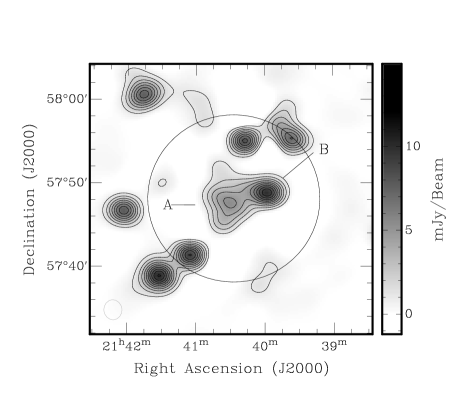
Since the frequency coverage of AMI tells us nothing about the spectral behaviour at longer radio wavelengths we must combine our new data with existing archival data. Ideally total power measurements are required, with the same or better angular resolution than AMI. Data of this type allow sampling in the plane to match exactly the measured angular scales of AMI. Here we use data from the Canadian Galactic Plane Survey (hereinafter CGPS; Taylor et al. 2003) at 1.42 GHz. These data are a combination of single-dish and synthesis data, and provide a total power measurement of this region with a resolution of . In order to mimic an AMI observation, these data are modulated by the primary beam of AMI before sampling in the plane to match the AMI coverage. These data are then processed in the same way as the true AMI visibilities to give the final sampled image. Fig. 2 shows the sampled data which result from matching the visibility coverage to AMI channel 4.
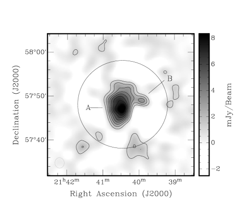
Spectra of both LDN 1111 and the radio source J213955+574859 are presented, identified as objects and respectively in Fig. 1. Errors on the data points in these spectra are calculated using a contribution for the rms noise in each channel, a conservative 5% flux calibration error and a contribution for the uncertainty in flux extraction. The morphology of LDN 1111 and its surroundings makes this extraction subject to the fitting area used. To account for this in the errors 10 independent ‘fits’ are made. The recorded flux density is the mean of these measurements and the variance is referred to as . These errors are combined in quadrature: . The flux extraction is performed using the fitflux program (Green 2007), which takes a user defined polygonal aperture and performs aperture photometry after subtracting a twisted plane background level. These errors are dominated by the 5% calibration uncertainty, with the map r.m.s. being 0.2 mJy per channel.
The spectrum of J213955+574859 is presented in order to demonstrate the flux calibration of AMI, see Fig. 3. The data points for this plot are given in Table 1. In addition to data points from the literature, flux densities at 408 MHz and 1.42 GHz from archival CGPS data are also plotted. These data have been extracted using the fitflux program as described above. Spectral indices are calculated using firstly the AMI data points plus the literature data, ; and secondly using all the data points, . These fits are shown as dot-dash and dashed lines respectively. Both are consistent with .
For J213955+574859, which is approximately point-like, we expect a negligible amount of flux loss from extended structure across the AMI bandwidth. In the case of LDN 1111 the same is not true. Using the CGPS map at 1.42 GHz we find 50% flux loss: the integrated flux from the original unsampled map, calculated as above, is mJy. However, since the morphology of the source varies between 1.4 and 16 GHz we have not used the CGPS data as a model to calculate flux loss.
Flux densities for LDN 1111 are listed in Table 2. It is immediately obvious that the flux densities for LDN 1111 between 14 and 18 GHz are inconsistent with an optically thin free–free spectrum extrapolated from 1.42 GHz. At the high frequency end of the AMI spectrum there is an excess of almost 50 mJy, .
Although an absolute measure of the flux loss is not feasible, it is possible to make an estimate of how the relative flux loss will affect the shape of the microwave spectrum. This is done using a multi-variate Gaussian model for the source with dimensions of the deconvolved source at 14.63 GHz (AMI channel 4) as given by the aips task jmfit, . This model is then sampled in using the exact coverage of the individual channels, and their flux loss relative to the lowest channel is recorded. We assume an uncertainty of 10% on the percentage flux loss and propagate the errors. The results of this calculation are shown in Fig. 4 and tabulated in Table 2. It should be noted that this is a conservative uncertainty and the relative flux loss will only be in error should the morphology change significantly between 14 and 17 GHz.
Fig. 4 includes a data point at 353 GHz (850 m) from the Scuba instrument (Visser, Richer & Chandler 2001) for illustartive purposes. This data point is uncorrected for flux loss. These Scuba data at 850 m are chopped at 2.5 arcmin and consequently we would assume that information on scales larger than this is lost. To correctly estimate the flux loss at this frequency we would require information on the morphology of the vibrational dust emission. Parker (1988), from whose paper the Scuba sample were selected, lists the dimensions of LDN 1111 as arcmin. A multivariate Gaussian model based on this data would suggest a flux loss of approximately 73%.
Source extraction methods applied to the WMAP data at 23–91 GHz (López-Caniego et al. 2007) are only able to give us upper limits on any compact emission towards LDN 1111, with the lowest limit being at 41 GHz, Jy. This value is consistent with the noise level at that frequency.

| Frequency | Flux density | Relative | Corrected |
|---|---|---|---|
| flux loss | flux density | ||
| (GHz) | (mJy) | (%) | (mJy) |
| 1.420a | 7.2 0.7 | - | 7.20.7 |
| 14.631 | 50.72.9 | - | 50.72.9 |
| 15.381 | 53.93.2 | 10 | 59.9 6.8 |
| 16.130 | 54.53.3 | 17 | 65.7 7.6 |
| 17.150 | 55.53.3 | 24 | 73.0 8.4 |
a sampled CGPS data point
3 Analysis
The emission seen between 14.63 and 17.15 GHz by AMI is clearly in excess of a simple free–free spectrum extrapolated from the CGPS data at 1.4 GHz. A number of possibilities may throw some light on the nature of this excess. The thermal (vibrational) dust spectrum of proto-planetary disks around T-Tauri stars is expected to extend into the cm-regime. In these circumstances grain growth has increased the population of cm-sized grains, or pebbles, causing to approach zero and the greybody spectrum to fall off with an index approaching 2. However the size of these disks is small and would be unlikely to be resolved by either AMI or Scuba. LDN 1111 is quite obviously elongated in the AMI data, as it is in the Scuba map which has a resolution of 14 arcsec. Although we do not deny the possibility of there being such a disk embedded within LDN 1111 or projected along the line of sight through this object, in the absence of further evidence we choose to pursue an alternative explanation.
A further possibility for a superposition of LDN 1111 and another object is that there may be an Hii region, with a density such that it is still optically thick at 16 GHz, whose flux is contributing to the spectrum. An Hii region with a turn-over frequency GHz, as would be required here, would possess an emission measure in excess of pc cm-6. This would put it in the regime of ultra-compact and hyper-compact Hii regions. The spectrum of these objects is inverted with an index of . The AMI data points alone have a spectral index of , rather steeper than would be expected. Indeed hyper-compact Hii regions exhibit slightly shallower spectra (Franco et al. 2000) which extends even to mm-wavelengths. The lack of a visible source in the WMAP data towards LDN 1111 would suggest that this is not the case here. In addition hyper-compact Hii regions tend to have very broad radio recombination line (RRL) widths, typically in excess of 50 km s-1 (Kurtz 2005). Ultra-compact Hii regions also show broadened line widths, of typically 30–40 km s-1. The RRL measurement of Heiles, Reach & Koo (1996) which encompasses LDN 1111 has a width of only 21.4 km s-1, although we note that this measurement is not directed at LDN 1111 specifically. An emission measure of this magnitude would also imply an Hii region mass of around 400 M⊙. The total mass of the cloud from the Scuba data (Visser et al. 2002) is 0.3 M⊙ only, which given the calculated flux loss in this data implies an upper limit on the mass of 1 M⊙.
A third possibility for the excess emission seen in the AMI data is that of dipole emission from rapidly rotating small dust grains (Drain & Lazarian 1998a,b). The observational evidence for this emission mechanism has been explored in the introduction to this letter. It is a relatively new emission mechanism and the evidence for its existence is not conclusive. We assess the possibility that the emission seen in LDN 1111 arises as a consequence of spinning dust by comparing the data to the model of Draine & Lazarian (1998a;b),which has been used extensively in the past. To make this comparison we use the MCMC based software metro (Hobson & Baldwin 2004) to find the best–fit parameters.
We fitted a model which has a free–free component normalized to give the flux density at 1.4 GHz from the sampled CGPS data with a spectral index of . To this we add a spinning dust component scaled from the DL98 molecular cloud model.
The model is parameterized by the column density, , and the angular size of the object. Visser et al. (2001) calculate the average and peak column densities for LDN 1111 as 5 and 13, respectively. The results of our model fitting are = 6.720.58, and = 5.380.26 arcmin. These values provide a of 1.03 (79% probability). However, given the small number of degrees of freedom in this case we do not propose this statistic as being conclusive. The resulting model is shown in Fig. 4. The column densities agree well with those of Visser et al., although as might be expected there is a degeneracy between the two parameters.

4 Discussion and Conclusions
Given the available evidence we propose the excess of emission we see towards the dark cloud LDN 1111 in the microwave band to be a result of emission from small spinning dust grains. This excess is quantified relative to a flux density derived from lower frequency data sampled to give the same coverage and consequently measuring the same angular scales on the sky. Lacking further data at lower frequencies with suitable angular resolution this one point is the basis for the assumption that there is an excess in the AMI frequency band. We therefore qualify this excess by using the original CGPS data to measure the total power, i.e. power on all scales, flux density at 1.42 GHz to be mJy. Since the object is extended this value may be regarded as an upper limit on the measureable flux at 1.42 GHz. In addition the total power CGPS data at 408 MHz may then be used to constrain better the lower frequency spectrum: mJy. The large error on this flux density is dominated by the fitting uncertainty. In combination these two flux densities yield a spectral index of , which predicts a total power flux at 16 GHz of mJy. This suggests that even in terms of total power there is a clear excess at 16 GHz.
Relative to a canonical free–free spectrum extrapolated from our sampled CGPS data at 1.42 GHz we see an excess of mJy, , assuming a fixed spectral index of . Using the spectral index derived from the CGPS total power maps at 408 MHz and 1.42 GHz then there is an excess of mJy, which is still .
In conclusion, we have presented observations of the Lynds’ dark nebula LDN 1111 at frequencies of 14.6–17.2 GHz. These measurements show an excess of emission towards this object relative to an extrapolated free–free spectrum at a significance of . We have proposed that this excess may be due to emission from small spinning dust grains and find that it is well-described by the model of Draine & Lazarian (1998a;b).
5 ACKNOWLEDGEMENTS
We thank the staff of the Lord’s Bridge observatory for their invaluable assistance in the commissioning and operation of the Arcminute Microkelvin Imager. We thank Nathalie Ysard and John Richer for useful discussions. We also thank Simon Casassus, whose comments and suggestions significantly improved this paper. The AMI is supported by Cambridge University and the STFC. NHW and MLD acknowledge the support of PPARC/STFC studentships.
References
- AMI Consortium: Zwart et al. (2008) AMI Consortium: Zwart J. T. L. et al., 2008, MNRAS in press, arXiv:0807.2469
- Baars et al. (1977) Baars J. W. M., Genzel R., Pauliny-Toth I. I. K., Witzel A., 1977, A&A, 61, 99
- Casassus, Readhead, Pearson, Nyman, Shepherd Bronfman (2004) Casassus S., Readhead A. C. S., Pearson T. J., Nyman L. -L., Shepherd M. C., Bronfman L., 2004, ApJ, 603, 599
- Casassus et al. (2006) Casassus S., Cabrera G. F., Förster F., Pearson T. J., Readhead A. C. S., Dickinson C., 2006, ApJ, 639, 951
- Casassus et al. (2008) Casassus S., et al., 2008, MNRAS in press, arXiv:0809.3965
- Condon et al. (1998) Condon J. J., Cotton W. D., Greisen E. W., Yin Q. F., Perley R. A., Taylor G. B., Broderick J. J., 1998, AJ, 115, 1693
- de Oliviera-Costa et al. (2002) de Oliviera-Costa A., et al., 2002, ApJ, 567, 363
- de Oliviera-Costa et al. (2004) de Oliviera-Costa A., Tegmark M., Davies R. D., Gutiérrez C. M., Lasenby A. N., Rebolo R., Watson R. A., 2004, ApJ, 606, L89
- Dickinson et al. (2006) Dickinson C., Casassus S., Pineda J. L., Pearson T. J., Readhead A. C. S., Davies R. D., 2006, ApJ, 643, L111
- Dickinson et al. (2007) Dickinson C., Davies R. D., Bronfman L., Casassus S., Davis R. J., Pearson T. J., Readhead A. C. S., Wilkinson P. N., 2007, MNRAS, 379, 297
- Dickinson et al. (2008) Dickinson C., et al., 2008, MNRAS in press, arXiv:0807.3985
- Draine & Lazarian (1998a) Draine B. T., Lazarian A., 1998a, ApJ, 494, L19
- Draine & Lazarian (1998a) Draine B. T., Lazarian A., 1998b, ApJ, 508, 157
- Ehman, Dixon, & Kraus (1970) Ehman J. R., Dixon R. S., Kraus J. D., 1970, AJ, 75, 351
- Finkbeiner (2004) Finkbeiner D. P., 2004, ApJ, 614, 186
- Finkbeiner et al. (2002) Finkbeiner D. P., Schlegel D. J., Frank C., Heiles C., 2002, ApJ, 566, 898
- Franco et al. (2000) Franco J., Kurtz S., Hofner P., Testi L., García-Segura G., Martos M., 2000, ApJ, 542, L143
- Green (2007) Green D. A., 2007, BASI, 35, 77
- Higgs (1971) Higgs L. A., 1971, MNRAS, 153, 315
- Hobson & Baldwin (2004) Hobson M. P., Baldwin J. E., 2004, Applied Optics, 43, 2651
- Jeffreys (1961) Jeffreys H., 1961, Theory of Probability, (Oxford: Clarendon Press)
- Kogut et al. (1996a) Kogut A., Banday A. J., Bennett C. L., Górski K. M., Hinshaw G., Reach W. T., 1996, ApJ, 460, 1
- Kogut et al. (1996b) Kogut A., Banday A. J., Bennett C. L., Górski K. M., Hinshaw G., Smoot G. F., Wright E. L., 1996, ApJ, 464, L5
- Kurtz (2005) Kurtz S., 2005, IAUS, 227, 111
- Leitch et al. (1997) Leitch E. M., Readhead A. C. S., Pearson T. J., Myers S. T., 1997, ApJ, 486, L23
- López-Caniego et al. (2007) López-Caniego M., González-Nuevo J., Herranz D., Massardi M., Sanz J. L., De Zotti G., Toffolatti L., Argüeso F., 2007, ApJS, 170, 108
- Parker (1988) Parker N. D., 1988, MNRAS, 235, 139
- Patnaik et al. (1992) Patnaik A. R., Browne I. W. A., Wilkinson P. N., Wrobel J. M., 1992, MNRAS, 254, 655
- Rengelink et al. (1997) Rengelink R. B., Tang Y., de Bruyn A. G., Miley G. K., Bremer M. N., Roettgering H. J. A., Bremer M. A. R., 1997, A&AS, 124, 259
- Scaife et al. (2007) Scaife A., et al., 2007, MNRAS, 377, L69
- Scaife et al. (2008) Scaife A. M. M., et al., 2008, MNRAS, 385, 809
- Sharpless (1959) Sharpless S., 1959, ApJS, 4, 257
- Taylor et al. (2003) Taylor A. R., et al., 2003, AJ, 125, 3145
- Visser, Richer, & Chandler (2001) Visser A. E., Richer J. S., Chandler C. J., 2001, MNRAS, 323, 257
- Wall, Wright, & Bolton (1976) Wall J. V., Wright A. E., Bolton J. G., 1976, AuJPA, 39, 1
- Watson et al. (2005) Watson R. A., et al., 2005, ApJ, 624, L89
- Wright et al. (2008) Wright E. L., et al., 2008, arXiv, arXiv:0803.0577