Magnetization Plateau of Classical Ising Model on Shastry-Sutherland Lattice

Abstract

We study the magnetization for the classical antiferromagnetic Ising model on the Shastry-Sutherland lattice using the tensor renormalization group approach. With this method, one can probe large spin systems with little finite-size effect. For a range of temperature and coupling constant, a single magnetization plateau at one third of the saturation value is found. We investigate the dependence of the plateau width on temperature and on the strength of magnetic frustration. Furthermore, the spin configuration of the plateau state at zero temperature is determined.

I Introduction

The frustrated spin systems have attracted much attention over last decades since very rich physics can appear in these systems. review_frustration Some interest in such systems is concentrated on fascinating sequence of magnetization plateaus at fractional values of the saturation magnetization, which was first observed in two-dimensional spin-gap material SrCu₂(BO₃)₂. SrCuBO This compound can be described well by spin-1/2 antiferromagnetic Heisenberg model on the frustrated Shastry-Sutherland lattice (or the orthogonal-dimer lattice), Shastry81 as shown in Fig. 1. Besides the previously discovered plateaus at $1/3$, $1/4$ and $1/8$ of the saturated magnetization, evidence in favor of more fractional magnetization plateaus down to values as small as $1/9$ has been reported recently. Sebastian07 ; Levy08 ; Takigawa07 Stimulated by the discovery of magnetization plateaus, various theoretical and experimental explorations have been devoted to the properties of the Shastry-Sutherland model in a magnetic field. Miyahara03 ; Dorier08 ; Schmidt08 ; Abendschein08

Similar phenomena of magnetization plateaus is also observed in rare-earth tetraborides RB₄. The magnetic ions of these compounds are again located on a lattice that is topologically equivalent to the Shastry-Sutherland lattice. Yoshii07 ; Yoshii08 ; Michimura06 ; Yoshii06 ; Iga07 ; Gabani08 ; Siemensmeyer08 In particular, magnetization plateaus at small fractional values ($1/7,1/9\dots$ of the saturation magnetization) are reported in the compound TmB₄. Gabani08 ; Siemensmeyer08 Because fully polarized state can be reached for experimentally accessible magnetic fields, this compound allows exploration of its complete magnetization process. Note that, due to large total magnetic moments of the magnetic ions, this compound can be considered as a classical system. Moreover, because of strong crystal field effects, the effective spin model for TmB₄ has been suggested to be described by the spin-1/2 Shastry-Sutherland model under strong Ising (or easy-axis) anisotropy. Siemensmeyer08 Thus, studying the Ising limit is the first step toward a complete understanding of the magnetization process for this material.

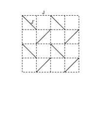
Figure 1: The Shastry-Sutherland lattice. $J$ bonds (dashed lines) are the exchange couplings along the edges of the squares and $J^{\prime}$ bonds (solid lines) are the diagonal intra-dimer couplings.

In the presence of a finite magnetic field $h$, the total energy of the antiferromagnetic Ising model on the Shastry-Sutherland lattice is given by

$$E(\{s_{i}\})=J\sum_{<i,j>}s_{i}s_{j}+J^{\prime}\sum_{\ll i,j\gg}s_{i}s_{j}-h\sum_{i}s_{i}\;,$$ (1)

with exchange couplings $J$, $J^{\prime}\geq 0$. Here, $s_{i}=\pm 1/2$ denotes the $z$-component of a spin-1/2 degree of freedom on site $i$ of the square lattice. The first sum extends over all nearest neighbor bonds, and the second sum runs over next-nearest neighbor bonds in every second square, as indicated in Fig. 1. Even for this simplified case, different conclusions for the magnetization curve have been reached. In Ref. Siemensmeyer08, , a single plateau at $1/2$ of the saturation magnetization is found based on analyzing a finite system with 16 spins only. However, when larger system sizes up to $18\times 18$ spins are considered, a distinct plateau at $1/3$ of the saturation magnetization is obtained. Meng08 The discrepancy may come from the effect of finite lattice sizes. As noted by the authors of Ref. Meng08, , for finite systems, inappropriate lattice sizes and boundary conditions can frustrate certain magnetization patterns, and hence lead to rather different magnetization curves which do not correctly represent the behavior in the thermodynamic limit. For example, the plateau at $1/3$ of the saturation magnetization is not allowed for systems of $4\times 4$ and $8\times 8$ spins, even though it does describe the true magnetization process for systems in the thermodynamic limit.

In order to check theoretically if other reported magnetization plateaus at small fractional values can be stabilized in the current model, unbiased large-scale calculations are called for. This is because the unit cells of magnetization profiles inside high-commensurability plateaus are usually quite large, calculations for systems of finite sizes may prevent reliable predictions for these cases. Therefore, to avoid the frustration for certain magnetization plateaus coming from geometric constraints, and in particular to uncover the possibility of plateaus at small fractional values, analyzing systems of large enough sizes are necessary.

Lately, based on ideas from quantum information theory, the tensor renormalization group (TRG) method is developed, Levin07 which can efficiently calculate quantities of classical systems of very large sizes. This technique can in principle be applied to any classical lattice with local interactions as long as the partition function can be expressed as a tensor network. Shi06 Because the accuracy can be systematically improved by increasing the cutoff on the index range of the tensors, highly precise quantities can be calculated under the TRG approach even in the thermodynamic limit. Levin07 ; Hinczewski08 ; Gu08 Therefore, the TRG method is one of the most suitable ways to study the magnetization process of the classical frustrated spin systems in the thermodynamical limit.

In the present work, the magnetization process of the spin-1/2 Shastry-Sutherland model in the Ising limit is investigated by employing the TRG approach. Levin07 ; Hinczewski08 ; Gu08 We find that the magnetization curve exhibits exactly one plateau at $1/3$ of the saturation value. Our results are in accordance with the findings in Ref. Meng08, . Furthermore, phase diagrams in the ($h,T$) plane for a typical magnetic coupling ratio $J^{\prime}/J=1$ and in the ($h,J^{\prime}$) plane for a particular temperature $T/J=0.2$ are obtained. Since there is no evidence for the presence of any additional plateaus for the spin-1/2 Shastry-Sutherland model in the Ising limit, to explain the experimental results, one must go beyond this simple model.

This paper is organized as follows. In Sec. II, the TRG approach is outlined briefly. In Sec. III, we apply this method to investigate the magnetization process of the Shastry-Sutherland model in the Ising limit. The spin configuration of the plateau state at zero temperature is discussed in Sec. IV. Sec. V is the conclusion.

II TRG formulation

Before applying the TRG method of Levin and Nave, Levin07 we first explain how to express the partition function of the present model as a tensor network. One possible way is to rewrite the total energy in Eq. (1) as a summation over the energies of plaquettes with diagonal bonds. note1 The energy of, say, the plaquette $A$ with spins $s_{1},s_{2},s_{3},s_{4}$ on its corners is given by (see Fig. 2)

$$\epsilon^{A}(s_{1},s_{2},s_{3},s_{4}) = J(s_{1}s_{2}+s_{2}s_{3}+s_{3}s_{4}+s_{4}s_{1})$$ (2)

$$+ J^{\prime}s_{2}s_{4}-\frac{h}{2}(s_{1}+s_{2}+s_{3}+s_{4})\;.$$

The rank-four tensors are defined as the Boltzmann weights for these plaquettes. For example,

$$T^{A}_{\alpha_{1},\alpha_{2},\alpha_{3},\alpha_{4}}=\exp[-\beta\epsilon^{A}(s_{1},s_{2},s_{3},s_{4})]$$ (3)

with $\beta$ being the inverse temperature and the indices $\alpha_{i}\equiv s_{i}+3/2$ running over 1 and 2. Afterwards, the partition function can be rewritten as a sum of tensor products in the following way,

$$Z = \sum_{\{s_{i}\}}e^{-\beta E(\{s_{i}\})}$$ (4)

$$= {\rm tTr}\left(T^{A}T^{B}\cdots\right)\;.$$

Here the tensor trace (tTr) means that all indices on the connected links in the tensor products are summed over. As a result, the partition function of the Ising model on the Shastry-Sutherland lattice is transformed to a tensor network as shown on the right-hand side of Fig. 2.

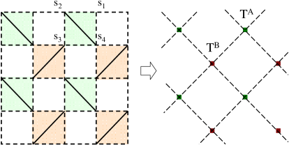
Figure 2: (Color online) Checkerboard decomposition of the Shastry-Sutherland lattice and the corresponding tensor network.

As discussed in Refs. Levin07, ; Hinczewski08, ; Gu08, , the tensor network can be coarse-grained in an iterative fashion to reduce the load of computation. At the mean time, the accuracy can be controlled by a parameter of cutoff $D_{cut}$. Here we outline the process briefly. Each step of the renormalization consists of two operations: rewiring and decimation. After one step of the renormalization, the number of sites in the tensor network is reduced by half. Eventually, the system is reduced to only four sites (four $T$’s) and the partition function can be calculated with ease.

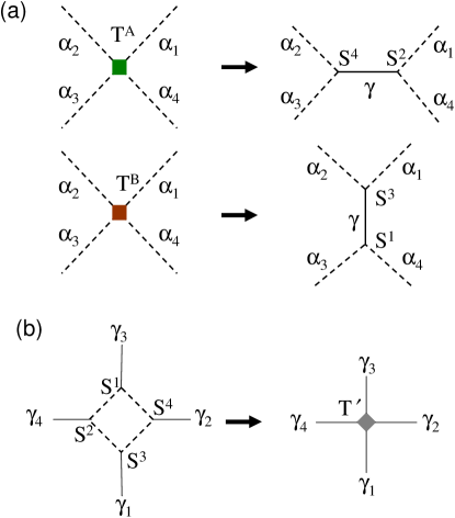
Figure 3: (a) Rewiring: the original rank-four tensors are decomposed to two rank-three tensors. (b) Decimation: the new tensor $T^{\prime}$ is obtained by summing over the indices around the square.

Rewiring – By viewing the rank-four tensor as a matrix, say $M_{(\alpha_{2},\alpha_{3}),(\alpha_{4},\alpha_{1})}=T^{A}_{\alpha_{1},\alpha_{2},\alpha_{3},\alpha_{4}}$, and with the help of singular value decomposition (SVD), $M=U\Lambda V^{\dagger}$, the rank-four tensor can be decomposed to two rank-three tensors. That is [see Fig. 3(a)],

$$T^{A}_{\alpha_{1},\alpha_{2},\alpha_{3},\alpha_{4}} = \sum_{\gamma=1}^{D^{2}}S^{4}_{(\alpha_{2},\alpha_{3}),\;\gamma}S^{2}_{(\alpha_{4},\alpha_{1}),\;\gamma}\;,$$

$$T^{B}_{\alpha_{1},\alpha_{2},\alpha_{3},\alpha_{4}} = \sum_{\gamma=1}^{D^{2}}S^{3}_{(\alpha_{1},\alpha_{2}),\;\gamma}S^{1}_{(\alpha_{3},\alpha_{4}),\;\gamma}\;.$$ (5)

Here $S^{4}_{(\alpha_{2},\alpha_{3}),\;\gamma}=\sqrt{\lambda_{\gamma}}U_{(\alpha_{2},\alpha_{3}),\;\gamma}$, $S^{2}_{(\alpha_{4},\alpha_{1}),\;\gamma}=\sqrt{\lambda_{\gamma}}V^{\dagger}_{\gamma,\;(\alpha_{4},\alpha_{1})}$ (similarly for $S^{3}$ and $S^{1}$), in which $\lambda_{\gamma}$ are the singular values, and $U$, $V$ are the unitary matrices in SVD. If each index of the original rank-four tensor has $D$ possible values, then there should be $D^{2}$ terms in the summation of Eq. (5). In practice, the tensor is approximated by keeping only the largest $D_{cut}$ singular values and the corresponding singular vectors. Apparently, the cutoff needs to be chosen such that the result converges with little $D_{cut}$-dependence.

Decimation – After rewiring, the dashed lines in Fig. 3(a) can be closed to build a new rank-four tensor, $T^{\prime}$ [see Fig. 3(b)]. This is achieved by the following operation,

$$T^{\prime}_{\gamma_{1},\gamma_{2},\gamma_{3},\gamma_{4}}={\rm Tr}\left(\textsf{S}^{4}_{\gamma_{2}}\textsf{S}^{3}_{\gamma_{1}}\textsf{S}^{2}_{\gamma_{4}}\textsf{S}^{1}_{\gamma_{3}}\right)\;,$$ (6)

where the square matrices $\left(\textsf{S}^{k}_{\gamma}\right)_{\alpha,\alpha^{\prime}}\equiv S^{k}_{(\alpha,\alpha^{\prime}),\gamma}$. After such a contraction, one obtains a new tensor network that is half of the size (see Fig. 4). Afterwards, the renormalization can be carried out iteratively until there are only four sites left.

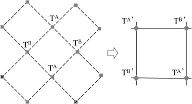
Figure 4: Under the TRG procedure, a tensor network is transformed into a coarse-grained tensor network.

We note that, to prevent the computation from diverging, one needs to normalize the new rank-four tensor at each step of the renormaliztion. At the beginning, we factor out the maximal value $W_{0}$ of the tensor elements of $T^{A/B}\equiv T^{A/B}_{0}$ to obtain a normalized tensor $\tilde{T}^{A/B}_{0}$. After the first step of the renormalization-group (RG) transformation on $\tilde{T}^{A/B}_{0}$, a renormalized tensor $T^{\prime}\equiv T_{1}$ is reached. Now we choose the normalization factor to be $W_{1}=\lambda^{A}_{max}\lambda^{B}_{max}$ such that $T_{1}=W_{1}\tilde{T}_{1}$, where $\lambda^{A}_{max}$ and $\lambda^{B}_{max}$ are the largest singular values of the two decompositions in Eq. (5).

The factorization and RG transformation are then iterated, so that at the $n$th step we have a tensor $T_{n}=W_{n}\tilde{T}_{n}$. Thus, for the Shastry-Sutherland lattice of $N=2^{n+3}$ sites (and with $N/2$ tensors in the original tensor network), after $n$ steps of the RG transformation, one has

$$Z = {\rm tTr}\left(T_{0}^{A}T_{0}^{B}\cdots T_{0}^{B}\right)$$ (7)

$$= W_{0}^{N/2}W_{1}^{N/4}\cdots W_{n}^{N/2^{n+1}}{\rm tTr}\left(\tilde{T}_{n}^{A}\tilde{T}_{n}^{B}\tilde{T}_{n}^{A}\tilde{T}_{n}^{B}\right)\;.$$

Since the last tensor-trace term in Eq. (7) remains finite, its contribution to the free energy can be neglected for a large enough system. The free energy per site thus becomes

$$f=-\frac{1}{\beta}\frac{\ln Z}{N}\simeq-\frac{1}{\beta}\sum_{i=0}^{n}\frac{1}{2^{i+1}}\ln W_{i}\;.$$ (8)

Once the free energy is obtained, one can proceed to calculate the magnetization. The results are shown and discussed in the following sections.

III Numerical results

In this section, we present the numerical results on the magnetization plateau and related phase diagrams. Throughout the region being explored, we find only one magnetization plateau at $m/m_{s}=1/3$, where $m$ denotes the magnetization and $m_{s}$ its saturation value. Unless otherwise mentioned, the size of the system is $2^{10}\times 2^{10}$ with periodic boundary condition. That is, the number of steps of the RG transformation in Eqs. (7) and (8) is $n=17$. The temperature $T$ and the strength of magnetic frustration $J^{\prime}$ are measured in units of $J$.

Fig. 5 is a typical diagram of the magnetization curves for $J^{\prime}=1$. The curves for three temperatures ($T=0.05$, $0.1$ and $0.15$) are shown. The size of the system is $2^{10}\times 2^{10}$ and the cutoff $D_{cut}=18$. Current result converges well against further increase of the system size and the cutoff. For example, for $T=0.05$, a larger system with $2^{15}\times 2^{15}$ ($D_{cut}=18$) yields a result agrees to the sixth decimal place for the most part of the curve. A larger cutoff $D_{cut}=24$ (system size $2^{10}\times 2^{10}$) shows similar accuracy. The result is slightly less accurate near the edges of the magnetization plateau but still shows no visible difference from the $T=0.05$ curve in Fig. 5. Compared to other methods, the TRG method is both accurate and efficient for very large systems.

Figure 5: Magnetization curves for three different temperatures. The size of the system is $2^{10}\times 2^{10}$. The parameters are $J^{\prime}=1$ and $D_{cut}=18$.

A more complete scan of the temperature can be found in Fig. 6(a). Over the whole range of calculation, there is only one plateau at $m/m_{s}=1/3$. Its width gradually shrinks to zero near temperature $T=0.18$. The corresponding phase diagram for the 1/3-plateau is shown in Fig. 6(b). The extent of the plateau is determined by the locations of maximum slope near its edges, which will be denoted as $h_{c,1}$ and $h_{c,2}$ for the lower and the higher critical fields respectively. In Fig. 6(b), we have added the theoretical critical fields $(h_{c,1},h_{c,2})=(1,5/2)$ at zero temperature (details later). One can see that the numerical result does extrapolate to the theoretical values as temperature decreases.

Figure 6: (a) Magnetization versus temperature $T$ and magnetic field $h$. The parameters are $J^{\prime}=1$ and $D_{cut}=18$. (b) Phase diagram of the magnetization plateau. The theoretical values of the critical fields at zero temperature are denoted by filled circles.

Figure 7: (a) Magnetization versus frustration $J^{\prime}$ and magnetic field $h$. The parameters are $T=0.2$ and $D_{cut}=18$. (b) Phase diagram of the magnetization plateau. Dashed lines are the theoretical phase boundaries at zero temperature.

In Fig. 7(a), we show another scan of the magnetization with respect to $J^{\prime}$ and $h$ at $T=0.2$. At this temperature, there is no plateau for small frustration. The plateau appears when $J^{\prime}$ is slightly larger than 1. One can see that the widths of the plateaus remain roughly the same for $J^{\prime}>2$. Their positions appear to shift linearly with respect to the strength of the frustration $J^{\prime}$. One can see this clearly in the phase diagram of Fig. 7(b). The plateaus are again determined by the locations of maximum slope. The characters of this phase diagram at finite temperature are inherited from its counterpart at zero temperature (details later), which is also plotted in Fig. 7(b) for comparison. The plateaus at zero temperature indeed exhibit a constant width at large frustration and a linear shift of the plateau position. Such a behavior will be explained in the next section.

IV Magnetization plateau at zero temperature

When the temperature is zero, the system is in the ground state. If the spin configuration of the ground state is known, then the Ising energy of the system can be calculated analytically. Afterwards, by comparing the ground state energies at different parameters, one can determine the phase boundaries in the parameter space. In this section, we will consider three regimes of magnetization: the unmagnetized state ($m=0$), the state of the $1/3$-plateau, and the fully-magnetized state ($m/m_{s}=1$). It will be shown that the phase boundaries being determined are consistent with the numerical results reported in Sec. III.

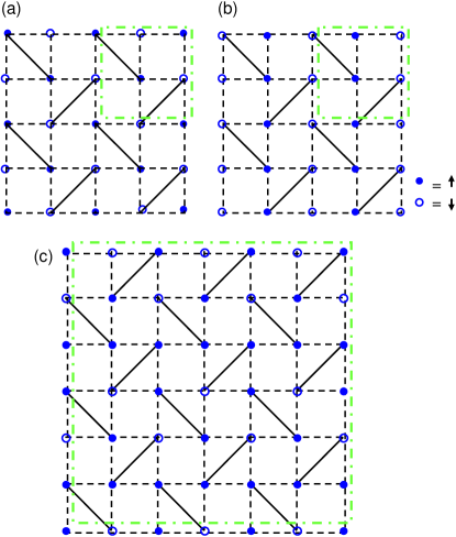
Figure 8: (Color online) (a) Spin configuration for the Néel state. (b) Spin configuration for the collinear state. (c) Spin configuration for the magnetization plateau at $m/m_{s}=1/3$. The squares with dashed-dotted lines indicate possible choices of unit cells.

In the unmagnetized state with $m=0$, we assume that the system is either in the Néel state or in the collinear state, depending on the strength of the frustration $J^{\prime}$. These states should be stable when the applied field $h$ is small. When the system is in the Néel state [Fig. 8(a)], for a unit cell formed by four plaquettes (bounded by dashed-dotted lines), there are two sites with spin up and two sites with spin down. The nearest-neighbor spins are all anti-parallel but the spins connected by the $J^{\prime}$-bond are parallel. It is not difficult to see that the energy per site, including the Zeeman energy (zero here), is,

$$\epsilon_{m=0}=-\frac{1}{2}+\frac{J^{\prime}}{8}\;,$$ (9)

in which $J=1$.

For large frustration, the system is more likely to be in the collinear state [Fig. 8(b)]. Again there are two up spins and two down spins in a unit cell of four plaquettes. Now the energy per site becomes

$${\tilde{\epsilon}}_{m=0}=-\frac{J^{\prime}}{8}\;.$$ (10)

By comparing the energies in Eqs. (9) and (10), one can see that the energy of the Néel state is lower (higher) than the collinear state when $J^{\prime}<2$ ($J^{\prime}>2$).

When the applied field increases, the system can undergo a phase transition to a $1/3$-plateau state. There are several possible candidates for such a state. In Fig. 8(c), we show the spin configuration of a state with the lowest possible energy. With careful analysis, one obtains the following spin energy per site,

$$\epsilon_{\frac{m}{m_{s}}=\frac{1}{3}}=-\frac{1}{6}-\frac{J^{\prime}}{24}-\frac{h}{6}\;.$$ (11)

When the applied field is sufficiently strong, then, irrespective of the value of $J^{\prime}$, the system should be fully magnetized. In such a case, it is relatively easy to determine the spin energy per site,

$$\epsilon_{\frac{m}{m_{s}}=1}=\frac{1}{2}+\frac{J^{\prime}}{8}-\frac{h}{2}\;.$$ (12)

By comparing $\epsilon_{m=0}$ and $\epsilon_{m/m_{s}=1/3}$, one can determine the boundary between the Néel state and the plateau state when $J^{\prime}<2$. The lower critical field $h_{c,1}$ is found to be

$$h_{c,1}=2-J^{\prime}\;.$$ (13)

Similarly, by comparing ${\tilde{\epsilon}}_{m=0}$ and $\epsilon_{m/m_{s}=1/3}$, one has the boundary between the collinear state and the plateau state when $J^{\prime}>2$,

$${\tilde{h}}_{c,1}=-1+\frac{J^{\prime}}{2}\;.$$ (14)

These two straight lines are indicated as the lower phase boundaries at zero temperature in Fig. 7(b).

On the other hand, the upper critical field $h_{c,2}$ is obtained by comparing the energies of the plateau state ($\epsilon_{m/m_{s}=1/3}$) and the fully magnetized state ($\epsilon_{m/m_{s}=1}$),

$$h_{c,2}=2+\frac{J^{\prime}}{2}\;.$$ (15)

Such a straight line is also shown in Fig. 7(b). The area bounded by these critical magnetic fields should be the maximum width of the plateau when the temperature of the system drops to zero. For example, when $J^{\prime}=1$, the plateau is bounded by $(h_{c,1},h_{c,2})=(1,5/2)$ at $T=0$. This agrees nicely with the extrapolation in Fig. 6(b).

V Conclusion

The TRG method is applied to explore the plateau in the magnetization process for the classical Ising model on the Shastry-Sutherland lattice. Systems as large as $2^{10}\times 2^{10}$ sites can be routinely studied with relative ease. Therefore, the complications from the finite-size effect and its related geometric frustration can essentially be avoided. We found a single plateau at $m/m_{s}=1/3$ that is robust over certain ranges of temperature and magnetic frustration, consistent with the result in Ref. Meng08, for smaller systems and higher temperatures. The model under investigation is relevant to the compound TmB₄, Siemensmeyer08 which is found to have a sequence of plateaus down to small fractional values. Gabani08 ; Siemensmeyer08 We note that the antiferromagnetic transverse exchanges have not been taken into account in the current classical model. Therefore, the quantum effect caused by these couplings may be essential in a full explanation of the observed plateaus.

- (1) Frustrated Spin Systems, edited by H. T. Diep (World Scientific, Singapore, 2004).
- (2) H. Kageyama, K. Yoshimura, R. Stern, N. Mushnikov, K. Onizuka, M. Kato, K. Kosuge, C. Slichter, T. Goto, and Y. Ueda, Phys. Rev. Lett. 82, 3168 (1999); K. Onisuka, H. Kageyama, Y. Narumi, K. Kindo, Y. Ueda, and T. Goto, J. Phys. Soc. Jpn. 69, 1016 (2000); H. Kageyama, Y. Ueda, Y. Narumi, K. Kindo, M. Kosaka, and Y. Uwatoko, Prog. Theor. Phys. Suppl. 145, 17 (2002); K. Kodama, M. Takigawa, M. Horvatić, C. Berthier, H. Kageyama, Y. Ueda, S. Miyahara, F. Becca and F. Mila, Science 298, 395 (2002).
- (3) B. S. Shastry and B. Sutherland, Physica B 108, 1069 (1981).
- (4) S. E. Sebastian, N. Harrison, P. Sengupta, C. D. Batista, S. Francoual, E. Palm, T. Murphy, N. Marcano, H. A. Dabkowska, and B. D. Gaulin, arXiv:0707.2075.
- (5) F. Levy, I. Sheikin, C. Berthier, M. Horvatic, M. Takigawa, H. Kageyama, T. Waki, and Y. Ueda, Europhys. Lett. 81, 67004 (2008).
- (6) M. Takigawa, S. Matsubara, M. Horvatic, C. Berthier, H. Kageyama, and Y. Ueda, Phys. Rev. Lett. 101, 037202 (2008).
- (7) For a review of earlier works, see S. Miyahara and K. Ueda, J. Phys.: Condens. Matter 15, R327 (2003), and references therein.
- (8) J. Dorier, K. P. Schmidt, and F. Mila, arXiv:0806.3406, to appear in Phys. Rev. Lett. (2008).
- (9) K. P. Schmidt, J. Dorier, and F. Mila, arXiv:0810.1596.
- (10) A. Abendschein and S. Capponi, arXiv:0807.1071, to appear in Phys. Rev. Lett. (2008)
- (11) S. Yoshii, T. Yamamoto, M. Hagiwara, T. Takeuchi, A. Shigekawa, S. Michimura, F. Iga, T. Takabatake, and K. Kindo, J. Magn. Magn. Mat. 310, 1282 (2007).
- (12) S. Yoshii, T. Yamamoto, M. Hagiwara, S. Michimura, A. Shigekawa, F. Iga, T. Takabatake, and K. Kindo, Phys. Rev. Lett. 101, 087202 (2008).
- (13) S. Michimura, A. Shigekawa, F. Iga, M. Sera, T. Takabatake, K. Ohoyama, and Y. Okabe, Physica B 378-380, 596 (2006).
- (14) S. Yoshii, T. Yamamoto, M. Hagiwara, A. Shigekawa, S. Michimura, F. Iga, T. Takabatake, and K. Kindo, J. Phys.: Conf. Series 51, 59 (2006).
- (15) F. Iga, A. Shigekawa, Y. Hasegawa, S. Michimura, T. Takabatake, S. Yoshii, T. Yamamoto, M. Hagiwara, and K. Kindo, J. Magn. Magn. Mat. 310, e443 (2007).
- (16) S. Gabani, S. Matas, P. Priputen, K. Flachbart, K. Siemensmeyer, E. Wulf, A. Evdokimova, and N. Shitsevalova, Acta Phys. Pol. A 113, 227 (2008).
- (17) K. Siemensmeyer, E. Wulf, H.-J. Mikeska, K. Flachbart, S. Gabani, S. Matas, P. Priputen, A. Evdokimova, and N. Shitsevalova, Phys. Rev. Lett. 101, 177201 (2008).
- (18) Z. Y. Meng and S. Wessel, arXiv:0808.3104.
- (19) M. Levin and C. P. Nave, Phys. Rev. Lett. 99, 120601 (2007).
- (20) Y.-Y. Shi, L.-M. Duan, and G. Vidal, Phys. Rev. A 74, 022320 (2006).
- (21) M. Hinczewski and A. Nihat Berker, Phys. Rev. E 77, 011104 (2008).
- (22) Z. C. Gu, M. Levin, and X. G. Wen, Phys. Rev. B 78, 205116 (2008).
- (23) Other constructions have also been suggested in the literature. For example, see F. Verstraete, M. M. Wolf, D. Perez-Garcia, and J. I. Cirac, Phys. Rev. Lett. 96, 220601 (2006); R. Orús and G. Vidal, Phys. Rev. B 78, 155117 (2008).