Discovery of Drifting High-frequency QPOs in Global Simulations of Magnetic Boundary Layers

Abstract

We report on the numerical discovery of quasi-periodic oscillations (QPOs) associated with accretion through a non-axisymmetric magnetic boundary layer in the unstable regime, when two ordered equatorial streams form and rotate synchronously at approximately the angular velocity of the inner disk The streams hit the star’s surface producing hot spots. Rotation of the spots leads to high-frequency QPOs. We performed a number of simulation runs for different magnetospheric sizes from small to tiny, and observed a definite correlation between the inner disk radius and the QPO frequency: the frequency is higher when the magnetosphere is smaller. In the stable regime a small magnetosphere forms and accretion through the usual funnel streams is observed, and the frequency of the star is expected to dominate the lightcurve. We performed exploratory investigations of the case in which the magnetosphere becomes negligibly small and the disk interacts with the star through an equatorial belt. We also performed investigation of somewhat larger magnetospheres where one or two ordered tongues may dominate over other chaotic tongues. In application to millisecond pulsars we obtain QPO frequencies in the range of 350 Hz to 990 Hz for one spot. The frequency associated with rotation of one spot may dominate if spots are not identical or antipodal. If the spots are similar and antipodal then the frequencies are twice as high. We show that variation of the accretion rate leads to drift of the QPO peak.

1 Introduction

In disk-accreting magnetized stars, disk-magnetosphere interaction and channeling of matter to the magnetic poles may determine the majority of observational features of such stars (e.g., Ghosh & Lamb, 1979; Königl, 1991). These include young solar-type stars (e.g., Bouvier et al., 2007) and very old stars such as magnetized white dwarfs (Warner, 1995) or accreting millisecond pulsars (van der Klis, 2000). In many cases no clear period is observed, and high-frequency quasi-periodic oscillations (QPOs) with a frequency corresponding to a fraction of the Keplerian frequency at the stellar surface are seen instead. It is often the case that a second, lower frequency peak appears and drifts in concert with the main frequency, forming two-peak QPOs. Such high-frequency oscillations are observed in both accreting millisecond pulsars (e.g., Wijnands & van der Klis, 1998) and in dwarf novae, which are a sub-class of cataclysmic variables (Woudt & Warner, 2002; Warner & Woudt, 2006). It has been suggested that the high-frequency QPOs may be associated with accretion to a star with a very weak magnetic field, when some sort of weakly magnetized equatorial belt forms (Paczyński, 1978; Warner & Woudt, 2002). Miller et al. (1998) and Lamb & Miller (2001) suggested that the high-frequency QPOs in accreting millisecond pulsars may result from rotation of clumps in the inner disk around a weakly magnetized star. They suggested that some of the disk matter may penetrate through the magnetosphere until stopped, e.g., by the radiation pressure. In this paper we investigate accretion to stars with small magnetospheres, where the energy density of the disk matter dominates up to very small distances from the star, or even up to the stellar surface, while magnetospheres are small compared to the radius of the star. We call the region around the star with a small magnetosphere the Magnetic Boundary Layer (MBL), and consider different cases. We notice that as for large magnetospheres, matter may accrete either in the stable (e.g., Romanova et al. 2003, 2004, hereafter RUKL03 and RUKL04) or unstable regime (Kulkarni & Romanova 2008a, b, hereafter KR08a,b; Romanova et al. 2008, hereafter RKL08). The most striking result is the fact that in the unstable regime, an ordered structure of two tongues forms, and rotates with the angular velocity of the inner disk, showing clear high-frequency QPO peaks associated with this rotation. Unstable accretion with a preferred number of tongues as a possible origin for QPOs has been discussed earlier by Li & Narayan (2004). In the present research we have shown that an even more ordered situation is possible with small magnetospheres, where two ordered tongues rotate with the frequency of the inner disk. Variation of the accretion rate leads to drifting of this QPO frequency. Correlation between the frequency and accretion rate has been observed in a number of accreting millisecond pulsars (e.g., van der Klis, 2000). Below we describe this and other results in detail. In §2 we discuss a possible classification scheme for magnetic boundary layers. In §3 we describe our model and reference parameters. In §4 we consider MBLs during stable accretion. In §5 we describe MBLs and formation of QPOs in the unstable regime. We present some discussion and conclusions in §6.

2 Classification of boundary layers

In accreting magnetized stars the disk is stopped by the stellar magnetosphere at the magnetospheric, or truncation, radius (e.g., Elsner & Lamb, 1977):

$$r_{m}=k_{A}({GM_{*}})^{-1/7}\dot{M}^{-2/7}\mu^{4/7},$$

where $M_{*}$ and $\mu$ are the mass and magnetic moment of the star, $\dot{M}$ is the accretion rate through the disk, and the coefficient $k_{A}$ is of the order of unity (e.g., Long et al., 2005; Bessolaz et al., 2008). The magnetospheric radius may be small if the magnetic moment of the star $\mu$ is small, or if the accretion rate is high. At a given magnetic moment of the star, variation of the accretion rate will lead to expansion or compression of the magnetosphere, and so at very high accretion rates the magnetosphere may be completely buried by accreting matter (e.g., Cumming et al., 2001; Lovelace et al., 2005), while at very low accretion rates it strongly expands, and different types of accretion are expected at different $\dot{M}$ (e.g., Romanova et al., 2008). An important parameter of the problem is the size of the magnetosphere in units of the stellar radius, $r_{m}/R_{*}$. Depending on this parameter we can define three types of boundary layers:

(1).  Hydrodynamic BL. If the ratio $r_{m}/R_{*}<<1$, then the magnetic field does not influence the dynamics of matter flow in the vicinity of the star, and a purely hydrodynamic boundary layer is expected where the magnetic field can be neglected. In this case the disk matter comes to the surface of the star and interacts with the star in the equatorial zone (e.g., Lynden-Bell & Pringle, 1974; Pringle, 1981; Popham & Narayan, 1995). Such interaction leads to release of a significant amount of energy at the surface of the star, about a half of the gravitational energy, $\dot{L}_{BL}\approx 0.5GM_{*}\dot{M}/R_{*}$. Interaction through such a hydrodynamic boundary layer is expected in many non-magnetic white dwarfs and neutron stars and in cases where accretion rate is so high that the magnetic field is buried by the accreting matter. It has been noted that the boundary layer matter will not interact with the star as a thin layer, but will spread to higher latitudes along the surface of the star due to matter pressure (Ferland et al., 1982). This effect has been calculated by Inogamov & Sunyaev (1999) and Piro & Bildsten (2004) and has recently been observed in axisymmetric hydrodynamic simulations by Fisker & Balsara (2005). Much less work has been done for analysis of the magnetic boundary layers (MBL).

(2).  Magnetic Boundary Layer (MBL) With Magnetospheric Gap. If the magnetosphere is only slightly larger than the radius of the star, $r_{m}/R_{*}>1$, then it stops the disk at a small distance from the star. The simulations described in this paper show that in this case, accretion may be either in the stable regime producing funnel streams, or in the unstable regime where most of the matter accretes through instabilities (KR08a; RKL08). We find that an unusual type of MBL forms in the unstable regime with two ordered streams rotating in the equatorial plane at approximately the angular velocity of the disk. These streams may be responsible for high-frequency QPOs.

(3). MBL Without a Magnetospheric Gap. If the magnetospheric radius is comparable to the stellar radius, $r_{m}/R_{*}\approx 1$, then the magnetosphere cannot stop the disk, and the disk interacts with the stellar surface. In this case the magnetic field may be somewhat enhanced in the accretion disk due to wrapping of the magnetic field lines by the disk matter. Preliminary simulations have shown that interesting phenomena may happen at the disk-magnetosphere boundary, such as interaction through a Kelvin-Helmholtz-type instability.

Global 3D simulations of accretion to stars with large magnetospheres (a few stellar radii in size) have been performed earlier (e.g., RUKL03,04; KR05). It was recently found that stars may be either in the stable or unstable regime of accretion (KR08a,b; RKL08). In this paper we show results of global 3D simulations of accretion to star with very small magnetospheres, in both stable and unstable regimes, and some results for direct interaction between the disk and the star.

3 Model

We solve the 3D MHD equations presented, e.g., in RUKL03, using the “cubed sphere” second order Godunov-type code described in Koldoba et al. (2002). The equations are written in a coordinate system rotating with a star. The energy equation is solved for the entropy, and the equation of state is that for an ideal gas. Viscosity is incorporated into the code with a viscosity coefficient proportional to $\alpha$ (Shakura & Sunyaev, 1973), where $\alpha<1$. The action of the viscosity is restricted to regions of high density (the disk). Viscosity helps bring matter towards the star from the disk.

3.1 Dimensionalization and Reference Values

The MHD equations are solved in dimensionless form so that the results can be readily applied to different types of stars. We have the freedom to choose three parameters from which the reference scales are derived, and we choose those to be the star’s mass $M$, radius $R_{*}$ and magnetic moment $\mu_{*}$ (with corresponding magnetic field $B_{*}=\mu_{*}/R_{*}^{3}$). We take the reference mass $M_{0}$ to be the mass $M$ of the star. The reference radius is about three times the radius of the star, $R_{0}=R_{*}/0.35\approx 3\times R_{*}$. In our past research (RUKL03; RUKL04) this radius approximately corresponded to the truncation (or magnetospheric) radius. In the present research the truncation radius is much smaller, but we keep this unit for consistency with our prior work. The reference velocity is $v_{0}=(GM/R_{0})^{1/2}$. The reference time-scale $t_{0}=R_{0}/v_{0}$, and the reference angular velocity $\omega_{0}=1/t_{0}$. We measure time in units of $P_{0}=2\pi t_{0}$ (which is the Keplerian rotation period at $r=R_{0}$). In the plots we use the dimensionless time $T=t/P_{0}$.

The reference magnetic moment $\mu_{0}=\mu_{*}/\widetilde{\mu}$, where $\widetilde{\mu}$ is a dimensionless parameter which determines the dimensionless size of the magnetosphere. The reference magnetic field is $B_{0}=\mu_{0}/R_{0}^{3}$. The reference density is $\rho_{0}=B_{0}^{2}/v_{0}^{2}$. The reference accretion rate is $\dot{M}_{0}=\rho_{0}v_{0}R_{0}^{2}$. Taking into account relationships for $\rho_{0}$, $B_{0}$, $v_{0}$ we obtain $\dot{M}_{0}=\mu_{*}^{2}/(\widetilde{\mu}^{2}v_{0}R_{0}^{4})$. The dimensional accretion rate is $\dot{M}=\widetilde{\dot{M}}\dot{M}_{0}$, where $\widetilde{\dot{M}}$ is the dimensionless accretion rate onto the surface of the star which is obtained from the simulations. Substituting parameters of the star to the reference values, we obtain the dimensional accretion rate:

$$\dot{M}=\bigg{(}\frac{\widetilde{\dot{M}}}{{\widetilde{\mu}}^{2}}\bigg{)}\frac{\mu_{*}^{2}}{(GM)^{1/2}(R_{*}/0.35)^{7/2}}.$$

One can see that at fixed parameters of the star ($M,R_{*},\mu_{*}$), the accretion rate depends on the ratio $\widetilde{\dot{M}}/{\widetilde{\mu}}^{2}$. Further analysis shows that parameter ${\widetilde{\mu}}^{2}$ varies more strongly than $\widetilde{\dot{M}}$ and determines the variation of the accretion rate. In the paper we vary parameter $\widetilde{\mu}$ which leads to variation of the dimensional accretion rate. Table 1 shows examples of reference variables for different stars. We solve the MHD equations using the normalized variables $\widetilde{\rho}=\rho/\rho_{0}$, $\widetilde{v}=v/v_{0}$, $\widetilde{B}=B/B_{0}$, etc. Most of the plots show the normalized variables (with the tildes implicit). To obtain dimensional values one needs to multiply values from the plots by the corresponding reference values from Table 1.

3.2 Initial and Boundary Conditions

Here we briefly summarize the initial and boundary conditions, described in detail in our earlier papers (e.g. in RUKL03). The simulation region consists of the accretion disk, the corona and the star. The star has a dipole magnetic field which is frozen into its surface. The disk is cold and dense. The corona is 100 times hotter and 100 times less dense (at the fiducial point at the inner edge of the disk). Initially we rotate the disk with Keplerian velocity and the star with the angular velocity of the inner disk, so as to avoid discontinuity of the magnetic field lines at the disk-star boundary. We also rotate the corona above the disk with the Keplerian velocity of the disk so as to avoid discontinuity at the disk-corona boundary. This is necessary since the discontinuity may lead to artificially strong forces on the disk and strong magnetic braking. In addition, we derive such a distribution of the density and pressure in the disk and corona, that the sum of the gravitational, pressure and centrifugal forces is equal to zero everywhere in the simulation region (Romanova et al., 2002). This initial condition ensures a very smooth gradual start-up, where the disk matter accretes slowly inwards due to viscous stresses. On the other hand, this condition dictates a density distribution that does not correspond to that in an equilibrium viscous disk (e.g. Shakura & Sunyaev, 1973). That is why our disk starts reconstructing itself on the viscous time-scale. Fortunately, matter from the inner parts of the disk flows inward for a long time, and the matter flux increases with $\alpha$, though dependence is not linear (as one would expect from the theoretical prediction for viscous disks). In addition, interaction of the disk with the external magnetosphere leads to some magnetic braking, leading to an enhancement of the accretion rate which may be smaller or larger than the effect of the viscosity and also to oscillations of the matter flux. That is why we cannot use the dimensionless accretion rate $\widetilde{\dot{M}}$ as a parameter of the problem. Instead, we choose $\widetilde{\mu}$ as the main parameter which is responsible for the size of the magnetosphere. Equation (1) shows that the dimensional accretion rate onto the star is regulated by the combination $\widetilde{\dot{M}}/{\widetilde{\mu}}^{2}$. In this paper we consider small magnetospheres with $\widetilde{\mu}\sim 0.08-0.5$, which is about 10 times smaller than in our past research (RUKL03; RUKL04; KR05).

The size of the simulation region is $R_{max}=15R_{0}\approx 45R_{*}$. We initially place the inner radius of the disk at a distance $r_{d}$ from the star which is either $1.2R_{0}\approx 3.6R_{*}$ (in stable cases) or $1.8R_{0}\approx 4.8R_{*}$ (in the unstable cases). Simulations show that the result does not depend on $r_{d}$, because in both cases the disk matter moves inward and is stopped by the magnetosphere at small distances from the star. Then we have the freedom to spin the star up or down gradually. In this paper we choose a slowly rotating star with angular velocity $\omega_{*}=(GM/r_{cor})^{1/2}$ corresponding to the corotation radius $r_{cor}=2R_{0}$. In dimensionless units, $\widetilde{\omega_{*}}=0.354$, and in application to neutron stars, $P_{*}=6.2$ms.

The boundary conditions are similar to those used in our other papers (e.g., RUKL03). On the star (the inner boundary) the magnetic field is frozen into the surface of the star (the normal component of the field, $B_{n}$, is fixed), though all three magnetic field components may vary. For all other variables $A$, free conditions are prescribed: $\partial A/\partial n=0$. The total velocity vector is adjusted to be parallel to the total magnetic field to enhance the frozen-in condition. At the external boundary, $r=R_{out}$, again free boundary conditions are prescribed for all variables. In some cases we fix the density on the external boundary so that matter of the disk stays in the region during the viscous reconstruction mentioned above. We do not supply matter to the disk from the external boundary, because the amount of matter in the inner regions of the disk is sufficient to support accretion over the duration of our simulations.

The grid. Simulations of accretion to stars with small magnetospheres require a finer grid compared to the larger magnetosphere cases (e.g. RUKL03). We use a grid resolution of $N_{r}\times N^{2}=100\times 41^{2}$ (in each of the 6 blocks of the cubed sphere) for most of our cases, and $N_{r}\times N^{2}=130\times 61^{2}$ for the smallest magnetospheres. The simulations were done using 60-180 processors each on the NASA HPC clusters.

4 Accretion in the stable regime

Below we describe the results of simulations of stable accretion to stars with small magnetospheres $\widetilde{\mu}=0.08-0.2$.

	CTTSs	White dwarfs	Neutron stars
$M(M_{\odot})$	0.8	1	1.4
$R_{*}$	$2R_{\odot}$	5000 km	10 km
$B_{*}$ (G)	$10^{3}$	$10^{6}$	$3\times 10^{8}$
$R_{0}$ (cm)	$4\times 10^{11}$	$1.4\times 10^{9}$	$2.9\times 10^{6}$
$v_{0}$ (cm s-1)	$1.6\times 10^{7}$	$3\times 10^{8}$	$8.1\times 10^{9}$
$\omega_{0}$ (s-1)	$4\times 10^{-5}$	0.21	$2.8\times 10^{3}$
$\nu_{0}$	$0.55$ day-1	$3.2\times 10^{-2}$ Hz	$4.5\times 10^{2}$ Hz
$P_{0}$	$1.8$ days	29 s	2.2 ms

Table 1: Sample reference values of the dynamical quantities for different types of stars. We choose the mass, radius and magnetic field of the star, and define the other variables in terms of these three quantities. Note that the frequency $\nu_{0}$ is the Keplerian frequency at radius $R_{0}$.

Simulations show that the boundary between the stable and unstable regimes depends on a number of factors, such as the accretion rate (determined by the viscosity parameter $\alpha$), the rotation period of the star $P_{*}$, and the misalignment angle $\Theta$ of the dipole (KR08a,b). If a star with a small misalignment angle, $\Theta<5^{\circ}$, rotates slowly (the disk rotates much faster than the star), then the accretion has a tendency to be unstable irrespective of $\alpha$ (KR08a,b). We have chosen slowly rotating stars with dimensionless angular velocity $widetilde{\omega_{*}}=0.354$ (corresponding to a corotation radius of $r_{cor}=2$). We take slowly rotating stars in order to model the situation in which the star initially has a large magnetosphere and is in the rotational equilibrium state, but later the accretion rate increases and the magnetosphere becomes small. To stabilize accretion we chose $\Theta=15^{\circ}$. We also used $\alpha=0.04$. In the description of the results we measure time in units of the Keplerian rotation period at $r=1$. We consider two main cases, one with $\widetilde{\mu}=0.2$ which has a small magnetosphere, and the other with $\widetilde{\mu}=0.08$ which has a tiny magnetosphere.

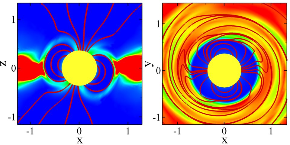
Figure 1: Stable accretion to a star with a small magnetosphere, where the magnetic moment of the star is $\widetilde{\mu}=0.2$ and is misaligned relative to the rotational axis $\Omega$ at $\Theta=15^{\circ}$. Left panel: Density distribution and sample magnetic field lines in the $xz$ ($\mu-\Omega$) plane. Right panel: The same, but in the $xy-$ (equatorial) plane. The dimensionless density varies between 0.8 (red) and 0.006 (blue).

Fig. 1 shows an example of accretion to a star with $\widetilde{\mu}=0.2$. A small magnetosphere forms, in which the magnetic field of the dipole dominates. The position of the inner disk edge is determined by the balance between the magnetic and kinetic matter pressure. Matter is lifted above the magnetosphere forming two funnel streams, and accretes to the surface of the star forming two hot spots. The hot spots show the distribution of the total energy flux on the surface of the star (see RUKL04 and KR05 for details).

The hot spots have a preferred position, although in case of small misalignment angles the funnel streams are dragged by the rapidly rotating disk and may rotate faster than the star. Such spot rotation has been observed in earlier simulations (RUKL03; Romanova et al. 2006). In the opposite situation when the star spins fast, both funnels and spots may rotate slower than the star (e.g. Romanova et al. 2002). Faster or slower rotation of spots may lead to a QPO feature with frequency higher or lower than the stellar frequency (Romanova et al. 2006). It has been suggested that at small misalignment angles, the spots may wander around the magnetic poles, possibly causing intermittency in some millisecond pulsars Lamb et al. (2008a,b) (see also (Altamirano et al., 2008; Casella et al., 2008)). On the other hand, if the misalignment angle of the dipole is not very small, then such faster or slower spot motions become less significant. The spots acquire a preferred place on the surface of the star and corotate with the star (see also RUKL03; RUKL04; KR05). In simulations with $\Theta=15^{\circ}$ we observe a mixture of spots: on the one hand, the disk drags the funnel around the weak magnetosphere in spite of the relatively high misalignment angle, and frame to frame analysis shows that the spots often move faster than the star. On the other hand, the hot spots spend a somewhat longer time in the $\mu-\Omega$ plane compared with other positions, due to which we observe a definite peak associated with star’s spin in the Fourier spectrum. Longer simulation runs are probably required to see the QPO peak.

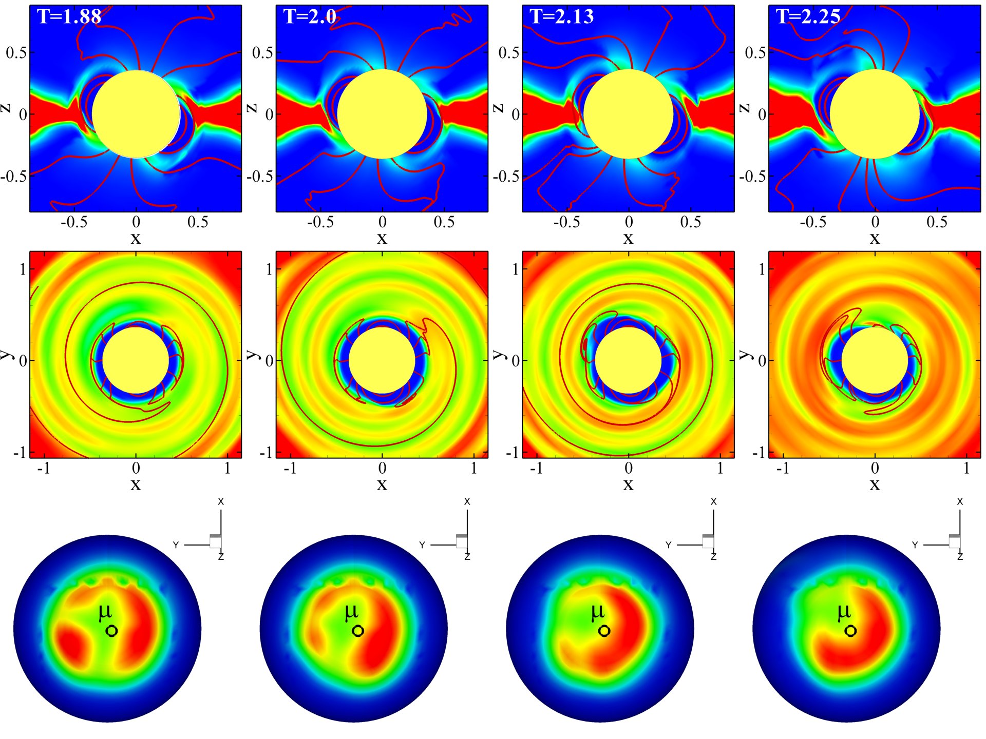
Figure 2: Stable accretion to a star with a very small (tiny) magnetosphere ($\widetilde{\mu}=0.08$) with $\Theta=15^{\circ}$ ($\alpha=0.04$). Top two panels: Density distribution and sample magnetic field lines in the $xz$ ($\mu-\Omega$) plane and the $xy-$ (equatorial) plane in a coordinate system rotating with the star. The dimensionless density varies between 1.4 (red) and 0.006 (blue). Bottom panel: Distribution of the dimensionless energy flux of matter onto the surface of the star (pole-on), varying between 0.4 (red) and 0.0009 (blue). The time $T$ is measured in units of $\Delta T=1/16P_{0}$, where $P_{0}$ is the Keplerian period at $r=1$.

Fig. 2 shows an example of accretion to a star with a tiny magnetosphere, $\widetilde{\mu}=0.08$. It is amazing that in this case too, the magnetosphere channels the accreting matter, forming tiny funnel streams hitting the surface of the star. Density waves form in the equatorial plane of the disk. Sometimes density fluctuations in the accreting matter push the disk to the stellar surface. However, later the magnetosphere is restored again. The hot spots have a preferred position but they often rotate faster than the star as a result of the difference in angular velocities between the disk and the star. In this case again, a QPO at the stellar frequency is expected, and also a QPO corresponding to the frequency at the inner edge of the disk and beats between these two frequencies. Longer simulation runs are required to extract these frequencies.

The main result of this section is that even small and tiny magnetospheres disrupt the disk and channel matter to the star, forming hot spots. It is also important to note that the high-frequency QPO associated with rotation of the inner edge of the disk is expected if the disk rotates faster (slower) than the star. Signs of faster rotation of the spot are clearly observed. Drifting of the high-frequency QPO is expected if the inner edge of the disk varies as a result of variation of the accretion rate. Future (longer) simulations will help obtain different frequencies.

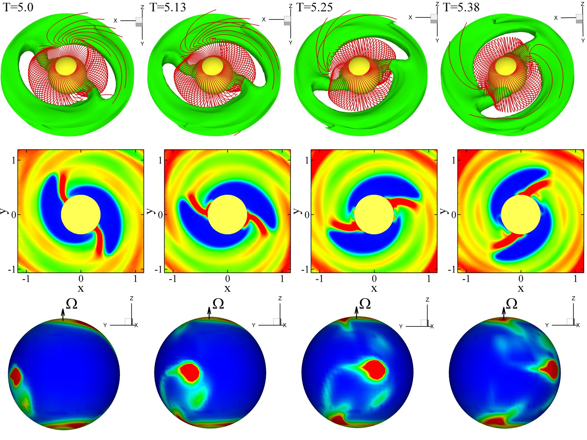
Figure 3: Snapshots of MBL accretion through the synchronized instability tongues in the case of a relatively large magnetosphere ($\widetilde{\mu}=0.2$ in dimensionless units). The time interval shown is a small portion of the simulation; the tongue pattern is steady for the entire duration of the simulation. Top panel: A surface of constant density (0.4 in dimensionless units) and sample magnetic field lines. Middle panel: Density distribution and sample magnetic field lines in the $xy$-plane. The density varies from 6.7 (red) to 0.01 (blue). Bottom panel: Energy flux onto the star’s surface, ranging from 3.4 (red) to 0.008 (blue). The figures are shown in a coordinate system rotating with the star. The time $T$ is measured in periods of Keplerian rotation at $r=1$.

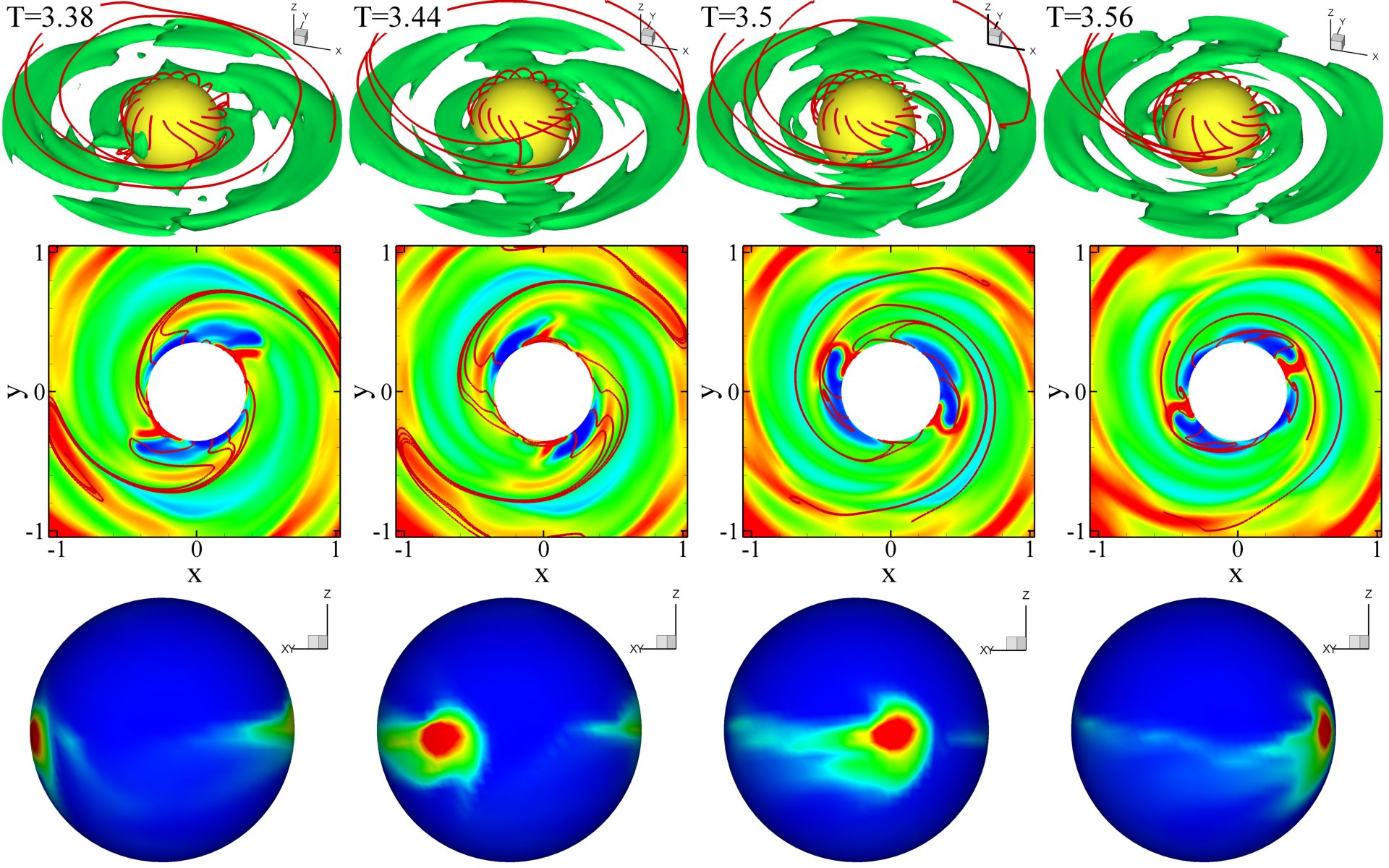
Figure 4: Top panel: A surface of constant density (0.47 in dimensionless units) and sample magnetic field lines in the case of a small magnetosphere, $\widetilde{\mu}=0.1$. Middle panel: $xy$-slice showing the density distribution and sample magnetic field lines. Bottom panel: density distribution on the surface of the star, ranging from 3.8 (red) to 0.01 (blue). The figures are shown in a coordinate system rotating with the star. The time $T$ is measured in periods of Keplerian rotation at $r=1$.

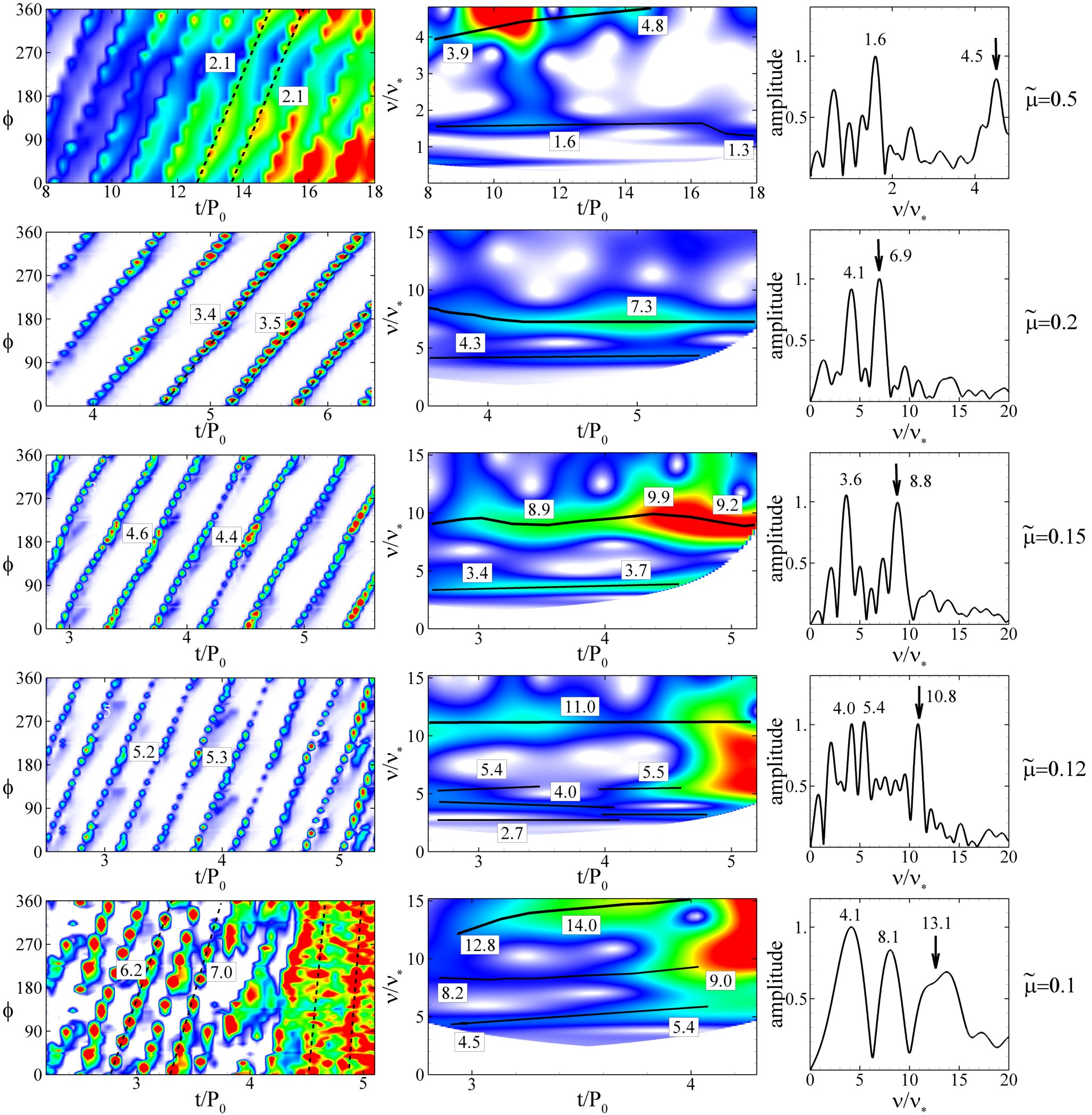
Figure 5: Frequency analysis for runs with different magnetospheric sizes. Left column: Spot-omega analysis showing the emitted energy flux distribution in the equatorial plane at different times. The flux varies from 3.4 (red) to 0.008 (blue). The lines reflect the motion of individual spots on the stellar surface. The slope of the lines is proportional to the angular velocity of the hot spots. Right two columns: Wavelet and Fourier spectra of the light curves from the hot spots obtained at an observer inclination angle of $i=90^{\circ}$ (i.e., when the observer is in the equatorial plane). The arrows show the frequency corresponding to the presence of two rotating spots. In the bottom row the lines show the distribution of the density, and not the flux, in the spots, and the density varies between 3.8 (red) and 0.01 (blue). In this case the lightcurve for which the wavelet and Fourier spectra are shown is calculated assuming that the emission of the star is proportional to the density.

5 Accretion in the unstable regime: A New Type of Boundary Layer and QPOs

5.1 Formation of two symmetric streams and spots

Now we take a star with a small misalignment angle, $\Theta=5^{\circ}$, and investigate accretion in the unstable regime. First we choose a small magnetosphere with magnetic moment $\widetilde{\mu}=0.2$. We take the viscosity coefficient $\alpha=0.1$ in all runs below. A star rotates slowly with angular velocity $\widetilde{\omega_{*}}=0.354$ (corresponding to $r_{cor}=2$). We observe that the instability starts, and matter penetrates through the equatorial region of the magnetosphere through a number of tongues. Later, however, two symmetric ordered tongues form and rotate synchronously with angular velocity approximately equal to the angular velocity in the inner region of the accretion disk, that is, much faster than the star. These tongues reach the surface of the star and produce two hot spots at the star’s equator which move faster than the star. The tongues deposit a significant amount of energy to the surface of the star. Part of this is the gravitational energy associated with acceleration of matter towards the star. We take this energy into account while plotting hot spots. In addition, there is energy released due to friction between the surface of the slowly rotating star and the foot-points of the rapidly rotating tongue.

Fig. 3 shows snapshots of rotation of the tongues, slices in the equatorial plane and hot spots (energy flux) on the star’s surface. The slices show that the magnetosphere has a strongly modified shape, particularly in those places where the tongues reach the surface of the star. They push the magnetosphere to the surface of the star and when the tongue moves, the magnetosphere re-emerges, while the tongue pushes another part of the magnetosphere to the surface of the star. Two strong hot spots form close to equatorial region. Sometimes they are not symmetric because the tongues push the magnetosphere more to one side than another. Some matter accretes to the poles through weak funnel streams. It is interesting that the polar spots also rotate with the angular velocity of the tongues. Thus, in the case of a small magnetosphere we observe a new phenomenon - a modified boundary layer, where the funnel streams and hot spots move with the angular velocity of the disk — much faster than the star. This is a new type of boundary layer where matter of the disk interacts with the star through unusual symmetric tongues. Rotation of the hot spots along the surface of the star is expected to give strong QPO peaks at twice the frequency of the inner disk.

To check this phenomenon, we performed a set of simulation runs at a variety of stellar magnetic moments: $\widetilde{\mu}=0.16$, $\widetilde{\mu}=0.15$, $\widetilde{\mu}=0.12$, $\widetilde{\mu}=0.1$, keeping all the other parameters fixed. We observed that similar symmetric streams form and rotate around the star. However, at smaller $\widetilde{\mu}$ the disk stops closer to the star. In the case of $\widetilde{\mu}=0.1$, only a tiny magnetosphere forms with tiny streams (see Fig. 4). The bottom panels of the Fig. 4 show the density distribution in the hot spots instead of the emitted flux, because it is expected that energy would be released mainly due to friction between the tongues and the surface of the star, which we do not calculate in this paper. In spite of the fact that the tongues are very small, there is still energy associated with gravitational acceleration of matter in the tongues and the corresponding heating of the stellar surface. The hot spots associated with gravitational acceleration are located in the regions of highest density and occupy a much smaller area than the spots shown in Fig. 4. At the end of the $\widetilde{\mu}=0.1$ simulation run the accretion rate increased, the disk reached the surface of the star and started interacting with the star’s surface through an equatorial belt (see §4.3).

We also performed exploratory simulations of accretion to stars with larger magnetospheres, $\widetilde{\mu}=0.5$ and observed that in many cases accretion through two or one ordered tongues dominates. We varied the $\alpha$ parameter (which regulates the accretion rate) and rotation rate of the star and obtained tongues and hot spots with different levels of order. In some cases two identical, diametrically opposite streams dominate accretion during the whole simulation run. In other cases only one stream dominates while the other is weaker, and therefore only one hot spot will determine the frequency observed in the light curve. In yet another type of case, multiple tongues are observed (like in cases of large magnetospheres, e.g. KR08a; KR08b), but one or two tongues are stronger than others, and can give rise to a QPO peak. Below we include the $\widetilde{\mu}=0.5$ case as an example of accretion to slightly larger magnetospheres. This case links the very small magnetospheres considered in this paper with the much larger ones considered in KR08b, where QPOs of similar origin are observed at some sets of parameters.

5.2 Frequency analysis

We performed frequency analysis for all the above cases. First we perform what we call spot-omega analysis, which we find to be the most informative for analysis of our simulations. Namely, we plot the equatorial distribution of the emitted energy flux at different moments of time (see Fig. 5, left column). We obtain diagonal lines which show that the spots have a definite order in their rotation along the star’s equator. The slopes of these lines are proportional to the angular velocity of the spots. We obtained a number of almost parallel lines which reflect multiple rotations of a single spot with approximately the same angular velocity. We performed this spot-omega analysis for all cases. Fig. 5 shows the spot-omega diagrams for the same time interval. One can see that at smaller $\widetilde{\mu}$, the lines are steeper because the inner disk is closer to the star and the rotation of the streams/spots is faster. Near the lines we show the rotation frequencies of the corresponding spots in units of the stellar rotation frequency. Note that in the case of the smallest magnetosphere ($\widetilde{\mu}=0.1$), the streams become very small and the spots associated with the energy flux due to gravitational acceleration become weak. In this case we plot the distribution of the density along the equator. Closer to the end of this simulation run, the disk comes to the surface of the star, and the streams (and ordered lines) disappear (see bottom left panel of Fig. 5). In the case of the largest magnetosphere, $\widetilde{\mu}=0.5$, the spot-omega diagram shows a little less order because the magnetosphere is stronger and the rotation of the tongues is less synchronized.

Next we performed wavelet analysis of the light-curves from hot spots. In the cases with $\widetilde{\mu}=0.5,0.2,0.15$ and $0.12$, the light-curve is calculated with the suggestion that all the gravitational and thermal energy of the matter falling onto the star is converted into thermal energy, which is radiated isotropically. The light from the surface of the star is integrated in the direction of the observer, whose line of sight makes an angle of $\i=90^{\circ}$ with the rotational axis of the star (see RUKL04 and KR05 for details). In the case with $\widetilde{\mu}=0.1$, it is expected that energy is released mainly due to friction between the rapidly moving streams and the star. Calculation of the radiation from such friction is beyond of the scope of this paper. As a first approximation we suggest that the emitted flux is proportional to the matter density at the star’s surface. Fig. 5 shows wavelet spectra for all these cases. These plots exclude early times, when the streams have yet to reach the star’s surface. Since the wavelet transform uses a window of width $\Delta t$ centered at time $t$ to calculate the time-dependent frequency spectrum of the lightcurve from time $t_{1}$ to time $t_{2}$, it is necessary to have $t_{1}+\Delta t/2\lesssim t\lesssim t_{2}-\Delta t/2$. This results in a portion of the wavelet plot being cut off. The width $\Delta t$ is inversely related to the frequency, so lower frequencies are more strongly affected by this restriction. One can see that in each case several frequencies are observed. Comparisons of the wavelet frequencies with the spot-omega frequencies (left panels) show that one of the frequencies is approximately twice as high as the frequency of the single spots shown in the spot-omega diagram, and hence corresponds to the motion of two spots along the surface of the star.

We also performed Fourier analysis of the light-curves. For this analysis we chose only the time intervals during which steady rotation of the spots was observed. In the case with $\widetilde{\mu}=0.1$, we also excluded the late times after the spots disappear and the boundary layer forms. The Fourier spectra show similar peaks as the wavelet. Between all these plots, the peak corresponding to rotation of two spots is most important. Thus we get an approximate agreement between the high-frequency QPOs obtained in all three methods of the frequency analysis.

There are also lower frequency peaks observed in both the wavelet and Fourier plots. These frequencies may either reflect the shape of the spots, or be beat frequencies (see also Smith et al., 1995; Psaltis et al., 1998). We do not see the star’s rotation frequency itself. However, it is possible that our simulations are not long enough for the wavelet analysis to capture possible QPOs associated with the slowly rotating star. On the other hand, the spot-omega diagrams do not show signs of stellar rotation, so it is possible that the corresponding QPO is very weak.

Note that spiral density waves often form in the disk (see Fig. 4, middle panels). The density waves tend to be stationary in the coordinate system rotating with a star, that is, they are generated by the inclination of the dipole. The rotating tongues disrupt the inner part of this pattern, but the external pattern approximately corotates with the star (see Fig. 4). The figure also shows that sample magnetic field lines starting out equidistantly from the star’s surface also accumulate in the density waves. Note that these density waves are similar in shape to those suggested by Miller et al. (1998), except that here the streams are guided by magnetic fields instead of being produced by radiation drag.

5.3 Interaction through the boundary layer

Closer to the end of the simulation run with the smallest magnetosphere ($\widetilde{\mu}=0.1$), the accretion rate increased and the disk matter started interacting with the surface of the star along a belt-like path (see Fig. 6). Later, the belt became wider, and an unusual pattern formed, connected with some instability. This is probably the Kelvin-Helmholtz instability which develops between the slowly rotating stellar surface and the much more rapidly rotating disk, which is expected to rotate at a frequency $\nu_{disk}\approx 8\nu_{*}$ at the surface of the star.

We should note that in all cases, when the modified tongue or a boundary layer reaches the surface of the star, it spreads to higher latitudes as it was predicted by Inogamov & Sunyaev (1999) (see also Piro & Bildsten, 2004; Fisker & Balsara, 2005). Fig. 7 shows such spreading and also a closer view of the unstable boundary layer on the star’s surface. During such close contact between the disk and the star, energy is expected to be released mainly from friction between the disk matter and the stellar surface, like in the usual hydrodynamic boundary layer. Compared to all the cases in the previous sections, no energy is associated with the matter falling onto the star’s surface. Such boundary layers require special investigation. Note that even in the case with no magnetosphere, a weak magnetic field threads the disk, and magnetic field lines are wrapped in the inner parts of the disk.

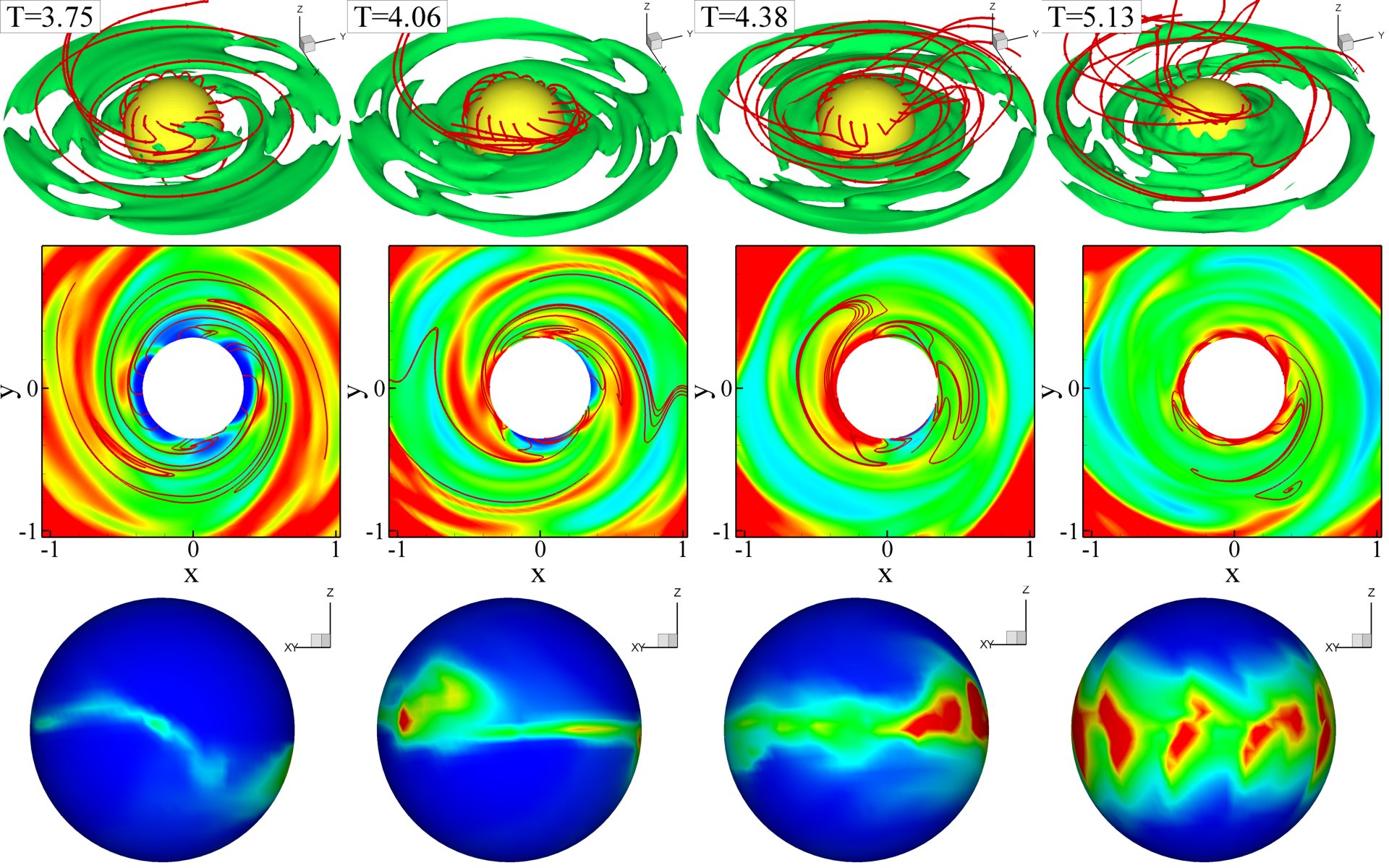
Figure 6: Same plot as in Fig. 4 but closer to the end of the run when the disk approaches the star. The surface shown in the top panels has a density of 0.43. In the bottom panels the density varies between 2.6 (red) and 0.007 (blue). The figures are shown in a coordinate system rotating with the star. The time $T$ is measured in periods of Keplerian rotation at $r=1$.

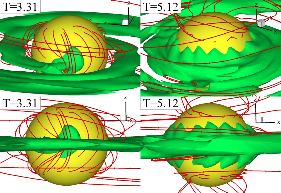
Figure 7: Enlarged view of two snapshots from Fig. 6, showing a surface of constant density (0.43 in dimensionless units) and sample magnetic field lines. The top and bottom panels show different projections. One can see that matter is lifted along the surface of the star to larger latitudes. In the case when the disk comes to the surface of the star, a new instability appears at the disk-star boundary, which is probably of the Kelvin-Helmholtz type.

At later times, when the disk comes closer to the star, the magnetic field lines trapped in the equatorial region are pushed closer to the star or buried. Note that at the same time the field lines above and below the disk are not buried (see also Fig. 7). Possibly the process of field burial by the thin disk through the boundary later should be reconsidered taking into account the fact that a significant amount of magnetic flux may inflate into the corona and stay there.

	$\widetilde{\mu}=0.5$	$\widetilde{\mu}=0.2$	$\widetilde{\mu}=0.16$	$\widetilde{\mu}=0.15$	$\widetilde{\mu}=0.12$	$\widetilde{\mu}=0.1$
$\widetilde{\dot{M}}/\widetilde{\mu}^{2}$	0.88	3.0	4.1	4.4	5.5	6
$\dot{M}$ ($M_{\odot}$yr-1)	$1.9\times 10^{-9}$	$6.6\times 10^{-9}$	$9.0\times 10^{-9}$	$9.7\times 10^{-9}$	$1.2\times 10^{-8}$	$1.3\times 10^{-8}$
$\nu_{1spot}$ (Hz)	350	541	670	715	843	986
$\nu_{2spot}$ (Hz)	700	1082	1340	1430	1686	1972

Table 2: Values of the quantities described in §5.4 as a function of the magnetospheric size parameter $\widetilde{\mu}$.

5.4 Example: Application to Accreting Millisecond Pulsars

Here we show a sample application of our simulations to accreting millisecond pulsars. We take a neutron star with mass $M_{*}=1.4M_{\odot}$, radius $R_{*}=10$ km and surface magnetic field $B_{*}=3\times 10^{8}$ G. The corresponding reference values are in Table 1. We convert the dimensionless results obtained in §4.1 and §4.2 into dimensional values. The dimensionless stellar angular velocity is $\widetilde{\omega_{*}}=0.354$. The corresponding dimensional angular velocity is $\omega_{*}=\widetilde{\omega_{*}}\omega_{0}=1002$ s^-1, dimensional period is $P_{*}=2\pi/\omega_{*}=6.3$ ms, and dimensional frequency is $\nu_{*}=159$ Hz. The time $T$ used in the figures has the reference value $P_{0}=2.2$ ms which is the Keplerian rotation period at $r=1$ ($3R_{*}=30$ km). The spot-omega diagrams in Fig. 5 (left panels) show the frequencies associated with the rotation of one spot for different values of $\widetilde{\mu}$. In the case of the larger magnetosphere ($\widetilde{\mu}=0.2$) the frequency is $\nu_{1spot}\approx 3.4\nu_{*}=541$ Hz. Since there are two antipodal hot spots, we expect the observer to see twice that frequency, $\nu_{2spots}\approx 1082$ Hz. In the case with $\widetilde{\mu}=0.15$, the disk is closer to the star and the frequencies are $\nu_{1spot}\approx 4.5\nu_{*}\approx 715$ Hz and $\nu_{2spots}\approx 1430$ Hz. For $\widetilde{\mu}=0.12$ the frequencies are $\nu_{1spot}\approx 5.3\nu_{*}=843$ Hz and $\nu_{2spots}\approx 1686$ Hz. And for $\widetilde{\mu}=0.1$ the frequencies are $\nu_{1spot}\approx 6.2\nu_{*}=986$ Hz and $\nu_{2spots}\approx 1972$ Hz. The frequencies are quite high because the disk is close to the surface of the star. In simulations with a larger magnetosphere, $\widetilde{\mu}=0.5$, we obtain lower frequencies, $\nu_{1spot}\approx 2.2\nu_{*}=350$ Hz and $\nu_{2spots}\approx 700$ Hz.

In application to neutron stars the formulae (1) can be re-written as:

$$\dot{M}=2.2\times 10^{-9}\bigg{(}\frac{\widetilde{\dot{M}}}{{\widetilde{\mu}}^{2}}\bigg{)}\bigg{(}\frac{B_{*}}{3\times 10^{8}{\rm G}}\bigg{)}^{2}$$

$$\bigg{(}\frac{M_{*}}{2.8\times 10^{33}{\rm g}}\bigg{)}^{-\frac{1}{2}}\bigg{(}\frac{R_{*}}{10^{6}{\rm cm}}\bigg{)}^{\frac{5}{2}}~{}\frac{\rm{\dot{M}_{\odot}}}{\rm yr}~{}.$$

One can see that the accretion rate depends on the dimensionless parameter $\widetilde{\dot{M}}/{\widetilde{\mu}}^{2}$. Table 2 shows that the ratio $\widetilde{\dot{M}}/{\widetilde{\mu}}^{2}$ decreases systematically with $\widetilde{\mu}$, and so do the accretion rate and the frequencies $\nu_{1spot}$ and $\nu_{2spots}$. So, the considered above cases with different $\widetilde{\mu}$ correspond to different accretion rates where, depending on accretion rate, the frequency drifts between $\nu_{2spots}\approx 700$ Hz when the accretion rate is lower and the magnetosphere is larger, and $\nu_{2spots}\approx 1972$ Hz when the accretion rate is higher and the magnetosphere is very small. The ratio between these two frequencies is 2.8 and can be smaller or possibly larger depending on the variation of the accretion rate, and is close to the observed drifts of the main high-frequency QPO in, e.g., millisecond pulsars (van der Klis, 2000) and dwarf novae (Warner & Woudt, 2006).

Only if the two hotspots are antipodal and identical, do we expect $\nu_{1spot}$ to be absent from the power spectrum. This is true for the small magnetosphere ($\widetilde{\mu}\leq 0.2$) cases. In the large magnetosphere ($\widetilde{\mu}=0.5$) case, we see that the spots are not identical; one spot is often much larger than the other, and hence the frequency $\nu_{1spot}$ may dominate. If the magnetic field of the star is not an ideal dipole field (that is, if it is a slightly misplaced dipole, or a more complex field (e.g., Long et al., 2007, 2008) then the symmetry breaks and one spot will be always larger than the others, and the lower frequency $\nu_{1spot}$ will dominate. Then we expected the frequency frift between 350 Hz and 990 Hz.

Simulations of stars with larger magnetosphere sizes, $\widetilde{\mu}\gtrsim 0.5$, usually show much more chaotic behavior in the unstable regime (KR08a,b; RKL08). In spite of stochastic accretion in the unstable regime, the spots on the surface of the star show a component which rotates with the angular velocity of the inner disk (KR08b). This component analyzed through rotation of spots (like in the left column of Fig. 5) shows clear inclination of lines associated with motion of different temporary spots with angular velocity approximately equal to the angular velocity of the inner disk (KR08a). This frequency component is weaker than the stochastic components associated with unstable accretion. However in longer simulation runs this QPO peak associated with the inner disk frequency may by amplified with time and may become significant, because the high-amplitude stochastic components are relatively incoherent and their frequencies constantly drift.

Although we consider accretion to a very slowly rotating star, similar MBLs and QPOs are expected for more rapidly rotating stars.

5.5 Disk oscillations

Note that some peaks observed in the wavelets and Fourier spectra may be associated with the disk-star interaction. An accretion disk can have different modes of oscillation. These include bending oscillations of the inner disk driven by the star’s rotating misaligned dipole field (e.g., Lai & Zhang, 2008) and radial oscillations of the inner disk (e.g., Alpar & Psaltis, 2008; Lovelace & Romanova, 2007; Lovelace et al., 2009; Erkut et al., 2008). The bending oscillations lead to the formation of an $m=1$ mode spiral wave rotating with the frequency of the star. In our simulations we do see traces of bending waves. The radial oscillations can arise from a linear Rossby wave instability (RWI) where the angular frequency of the oscillations (with mode number $m=1$) is less than the peak in the angular velocity in the inner disk, $\Omega_{\rm max}$ (Lovelace & Romanova, 2007; Lovelace et al., 2009). This mode is radially trapped in a narrow region inside the radius at which $\Omega_{\rm max}$ occurs. The beat between this mode and the stellar rotation frequency may lead to the coupled twin peak QPOs observed in some millisecond pulsars (e.g., van der Klis, 2006).

Here we derive from our simulations the radius at which the disk angular velocity matches that of the spot. Fig. 8 shows this analysis for cases with different $\widetilde{\mu}$. First, we plot the radial dependence of the angular velocity in the disk at sample times (see the top panels of the Fig. 8). Then we take the angular velocity of the spot from the spot-omega diagram (Fig. 5, left panels) and find the point where angular velocity of the spot equals the angular velocity in the disk (see red dots). Next, we plot the radial dependence of angular momentum (Fig. 8 middle panels) and density (bottom panels) at same moment of time. The circular line in the plots is the line on which the angular velocity equals that of the spot. One can see that in all cases the rotational velocity of the spot corresponds to the inner edge of the disk. It corresponds to a distance only slightly larger than the Alfvén surface (red line), where the kinetic plasma parameter $\beta_{1}=(p+\rho v^{2})/(B^{2}/8\pi)=1$. Note that the magnetosphere is strongly non-axisymmetric, and therefore the $\Omega$ distribution in the disk varies with time.

Different oscillation modes in the disk may influence the position or brightness variation of the spots on the surface of the star. We do observe some frequencies in the power spectra of the light-curves, but at present we are not sure that the observed frequencies reflect disk oscillations. Future (longer) simulation runs may help reveal such a possibility. On the other hand, disk oscillations can be investigated directly from the simulations. We plan to do this in the future.

Fig. 5 shows that there are several peaks observed in the wavelet and Fourier spectra. We know the origin of only one of them, associated with rotation of the unstable tongues. Other peaks may be associated with disk oscillations or with beat frequencies between the disk and the star. However, at present our runs are not long enough to establish the origin of these peaks.

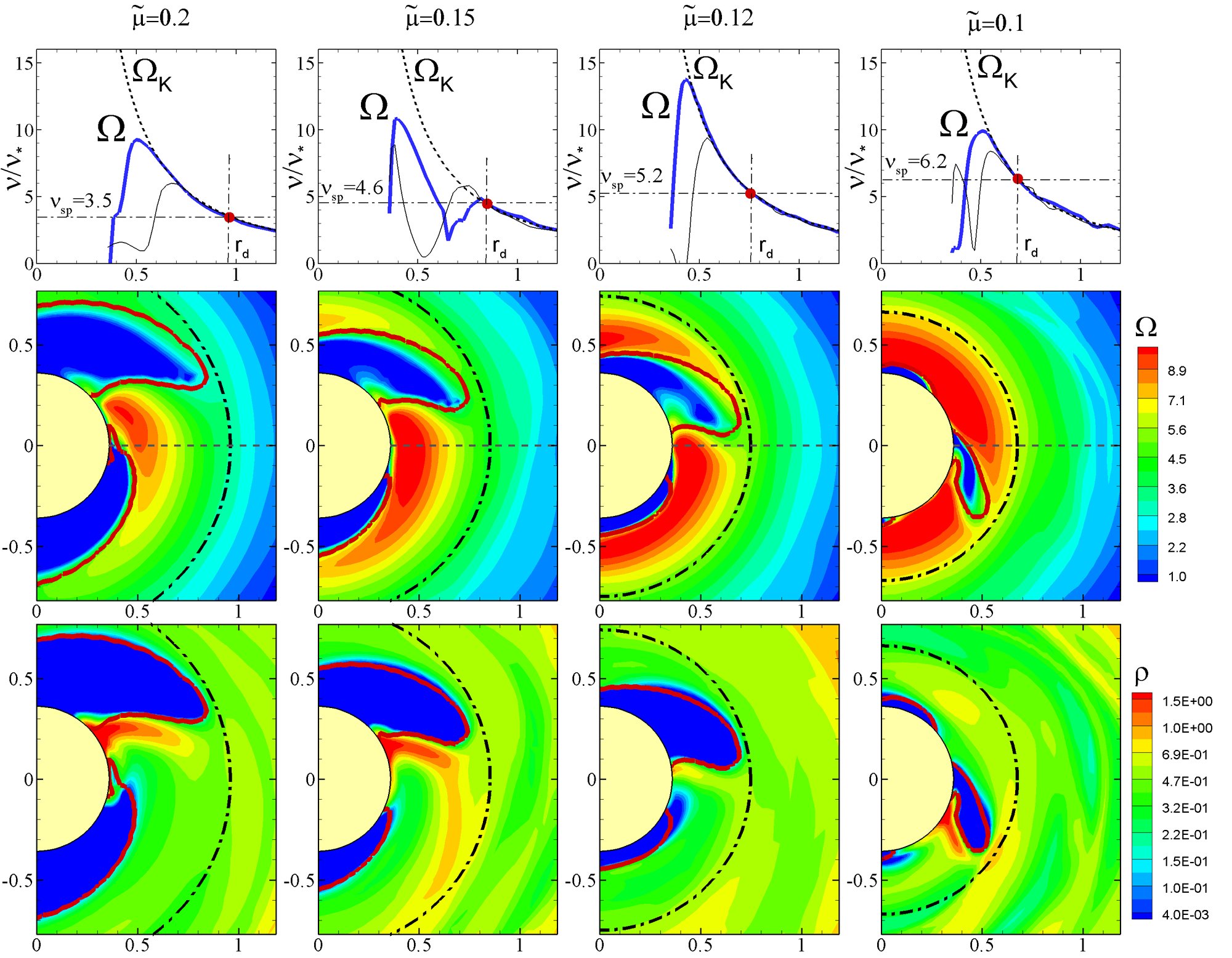
Figure 8: Top panels: Radial dependence of the disk angular velocity for the moments of time corresponding to the lower panels (thick blue line) and for other moments of time (black line). The red spot marks the point where the angular velocity matches that of the spots. Middle panel: Angular velocity distribution. The background shows the angular velocity, while the foreground shows the kinetic plasma parameter $\beta_{1}=1$ (red thick line) and the circle shows where the angular velocity equals that of the spot (black dash-dot line). Bottom panels: Same, but for the density distribution.

6 Conclusions

We considered accretion to slowly rotating stars with small and tiny magnetospheres in the stable and unstable regimes. We conclude that:

(1) In the stable regime, a small magnetospheric cavity and tiny funnel streams form, producing hot spots on the star’s surface which tend to be in a preferred position determined by the dipole inclination (we had example runs for $\Theta=15^{\circ}$). In this case the frequency of the star is expected to dominate. However, the rapidly rotating disk has a tendency to “drag” the funnel stream to faster rotation, due to which parts of the hot spots often rotate much faster than the star. At lower $\Theta$ this effect becomes even more significant, and the spots may rotate faster than the star for a long time, leading to QPOs (see also RUKL04), or slower than the star leading to matter accreting through a trailing funnel, (e.g., Romanova et al. 2002) producing a lower-frequency QPO.

(2) In the unstable regime we observed that matter accretes through two ordered streams which rotate with the angular velocity of the inner disk, that is, much faster than the star. They hit the surface of the star forming two antipodal hot spots. Rotation of these spots along the surface of the star leads to high-frequency QPOs. Such persistent streams/spots have been observed at a variety of parameters and are seen to be quite long-lived. Coherent rotation of this kind has been observed for small magnetospheres. For large magnetospheres we find that the spots are much more chaotic in the sense that they form at different parts of the star (RKL08; KR08a). In intermediate cases we observed that one or two ordered streams may form, which are less ordered than in the cases of small magnetospheres, but still may give QPO peaks (KR08b). On the other hand, the accretion may be stochastic, but one or two streams may be stronger than the others, and the hot spots associated with these streams may lead to QPOs.

(3) Correlation is observed between the size of the magnetosphere and the QPO frequency: the frequency is higher at smaller magnetospheric sizes. We expect that secular variation of the accretion rate will lead to drifting of the QPO frequency. Correlation between the frequency and the accretion rate has been observed in a number of accreting millisecond pulsars (e.g., van der Klis, 2000).

(4) We were able to model a wide range of QPO frequencies. In application to millisecond pulsars the frequency associated with rotation of one spot varies between $\nu_{1spot}=350$ Hz and $990$ Hz. In cases of small magnetospheres, the two spots are very similar in brightness, and the expected frequencies are twice as high. Only if the two spots are antipodal and identical, do we expect $\nu_{1spot}$ to be absent from the power spectrum. This is true for the small magnetosphere ($\widetilde{\mu}\leq$ 0.2) cases. In the large magnetosphere ($\widetilde{\mu}$=0.5) case, we expect to see $\nu_{1spot}$.

The most striking result of this paper is the discovery of a new regime of unstable accretion which shows clear high-frequency QPO peaks.

Acknowledgments

The authors thank R.V.E. Lovelace for discussions and the referee M.A. Alpar for comments and suggestions which helped improve the paper. The authors were supported in part by NASA grant NNX08AH25G and by NSF grants AST-0607135 and AST-0807129. We are thankful to NASA for using NASA High Performance Facilities.

References

- Alpar & Psaltis (2008) Alpar M. A., Psaltis D., 2008, MNRAS, 391, 1472
- Altamirano et al. (2008) Altamirano D., Casella P., Patruno A., Wijnands R., van der Klis M., 2008, ApJL, 674, L45
- Bessolaz et al. (2008) Bessolaz N., Zanni C., Ferreira J., Keppens R., Bouvier J., 2008, A&A, 478, 155
- Bouvier et al. (2007) Bouvier J., Alencar S. H. P., Harries T. J., Johns-Krull C. M., Romanova M. M., 2007, in Reipurth B., Jewitt D., Keil K., eds, Protostars and Planets V Magnetospheric Accretion in Classical T Tauri Stars. pp 479–494
- Casella et al. (2008) Casella P., Altamirano D., Patruno A., Wijnands R., van der Klis M., 2008, ApJL, 674, L41
- Cumming et al. (2001) Cumming A., Zweibel E., Bildsten L., 2001, ApJ, 557, 958
- Elsner & Lamb (1977) Elsner R. F., Lamb F. K., 1977, ApJ, 215, 897
- Erkut et al. (2008) Erkut M. H., Psaltis D., Alpar M. A., 2008, ApJ, 687, 1220
- Ferland et al. (1982) Ferland G. J., Pepper G. H., Langer S. H., MacDonald J., Truran J. W., Shaviv G., 1982, ApJL, 262, L53
- Fisker & Balsara (2005) Fisker J. L., Balsara D. S., 2005, ApJL, 635, L69
- Ghosh & Lamb (1979) Ghosh P., Lamb F. K., 1979, ApJ, 232, 259
- Inogamov & Sunyaev (1999) Inogamov N. A., Sunyaev R. A., 1999, Astronomy Letters, 25, 269
- Koldoba et al. (2002) Koldoba A. V., Romanova M. M., Ustyugova G. V., Lovelace R. V. E., 2002, ApJL, 576, L53
- Königl (1991) Königl A., 1991, ApJL, 370, L39
- Kulkarni & Romanova (2008a) Kulkarni A. K., Romanova M. M., 2008a, MNRAS, 386, 673
- Kulkarni & Romanova (2008b) Kulkarni A. K., Romanova M. M., 2008b, MNRAS, in press
- Lai & Zhang (2008) Lai D., Zhang H., 2008, ApJ, 683, 949
- Lamb et al. (2008) Lamb F. K., Boutloukos S., Van Wassenhove S., Chamberlain R. T., Lo K. H., Clare A., Yu W., Miller M. C., 2008, ArXiv e-prints
- Lamb et al. (2008) Lamb F. K., Boutloukos S., Van Wassenhove S., Chamberlain R. T., Lo K. H., Miller M. C., 2008, ArXiv e-prints
- Lamb & Miller (2001) Lamb F. K., Miller M. C., 2001, ApJ, 554, 1210
- Li & Narayan (2004) Li L.-X., Narayan R., 2004, ApJ, 601, 414
- Long et al. (2005) Long M., Romanova M. M., Lovelace R. V. E., 2005, ApJ, 634, 1214
- Long et al. (2007) Long M., Romanova M. M., Lovelace R. V. E., 2007, MNRAS, 374, 436
- Long et al. (2008) Long M., Romanova M. M., Lovelace R. V. E., 2008, MNRAS, 386, 1274
- Lovelace & Romanova (2007) Lovelace R. V. E., Romanova M. M., 2007, ApJL, 670, L13
- Lovelace et al. (2005) Lovelace R. V. E., Romanova M. M., Bisnovatyi-Kogan G. S., 2005, ApJ, 625, 957
- Lovelace et al. (2009) Lovelace R. V. E., Turner L., Romanova M. M., 2009, ArXiv e-prints
- Lynden-Bell & Pringle (1974) Lynden-Bell D., Pringle J. E., 1974, MNRAS, 168, 603
- Miller et al. (1998) Miller M. C., Lamb F. K., Psaltis D., 1998, ApJ, 508, 791
- Paczyński (1978) Paczyński B., 1978, in Zytkov, A., ed., Nonstationary Evolution of Close Binaries. PWN – Polish Scientific Publishers, Warsaw
- Piro & Bildsten (2004) Piro A. L., Bildsten L., 2004, ApJ, 610, 977
- Popham & Narayan (1995) Popham R., Narayan R., 1995, ApJ, 442, 337
- Pringle (1981) Pringle J. E., 1981, ARA&A, 19, 137
- Psaltis et al. (1998) Psaltis D., Mendez M., Wijnands R., Homan J., Jonker P. G., van der Klis M., Lamb F. K., Kuulkers E., van Paradijs J., Lewin W. H. G., 1998, ApJL, 501, L95+
- Romanova et al. (2006) Romanova M. M., Kulkarni A., Long M., Lovelace R. V. E., Wick J. V., Ustyugova G. V., Koldoba A. V., 2006, Advances in Space Research, 38, 2887
- Romanova et al. (2008) Romanova M. M., Kulkarni A. K., Long M., Lovelace R. V. E., 2008, in Wijnands R., ed., A Decade of Accreting Millisecond X-ray Pulsars Modeling of Disk-Star Interaction: Different Regimes of Accretion and Variability. pp 87–94
- Romanova et al. (2008) Romanova M. M., Kulkarni A. K., Lovelace R. V. E., 2008, ApJL, 673, L171
- Romanova et al. (2002) Romanova M. M., Ustyugova G. V., Koldoba A. V., Lovelace R. V. E., 2002, ApJ, 578, 420
- Romanova et al. (2004) Romanova M. M., Ustyugova G. V., Koldoba A. V., Lovelace R. V. E., 2004, ApJ, 610, 920
- Romanova et al. (2003) Romanova M. M., Ustyugova G. V., Koldoba A. V., Wick J. V., Lovelace R. V. E., 2003, ApJ, 595, 1009
- Shakura & Sunyaev (1973) Shakura N. I., Sunyaev R. A., 1973, A&A, 24, 337
- Smith et al. (1995) Smith K. W., Lewis G. F., Bonnell I. A., 1995, MNRAS, 276, L5
- van der Klis (2000) van der Klis M., 2000, ARA&A, 38, 717
- van der Klis (2006) van der Klis M., 2006, Rapid X-ray Variability. pp 39–112
- Warner (1995) Warner B., 1995, Cataclysmic variable stars. Cambridge Astrophysics Series, Cambridge, New York: Cambridge University Press, —c1995
- Warner & Woudt (2002) Warner B., Woudt P. A., 2002, MNRAS, 335, 84
- Warner & Woudt (2006) Warner B., Woudt P. A., 2006, MNRAS, 367, 1562
- Wijnands & van der Klis (1998) Wijnands R., van der Klis M., 1998, Nature, 394, 344
- Woudt & Warner (2002) Woudt P. A., Warner B., 2002, MNRAS, 333, 411