Anomalies in electrostatic calibrations for the
measurement of the Casimir force in a sphere-plane geometry

Abstract

We have performed precision electrostatic calibrations in the sphere-plane geometry, and observed anomalous behavior. Namely, the scaling exponent of the electrostatic signal with distance was found to be smaller than expected on the basis of the pure Coulombian contribution, and the residual potential found to be distance dependent. We argue that these findings affect the accuracy of the electrostatic calibrations and invite reanalysis of previous determinations of the Casimir force.

Over the last decades the Casimir force Casimir has met increasing popularity as a macroscopic manifestation of quantum vacuum Milonni , with its relevance spanning from nanotechnology to cosmology Bordag . With the claimed accuracy of recent experiments ranging from 15$\%$ in the parallel plane case Bressi to 0.1-5$\%$ in the sphere-plane case Lamoreaux ; Mohideen ; Chan ; Decca , it also provides constraints on the existence of forces superimposed to the Newtonian gravitational force and expected in various unification attempts Fishbach ; Onofrio .

Concern has been raised that previous analyses in the measurement of the Casimir force have overlooked possible influence of residual electric effects (the so-called patch effects), which could mimic the Casimir force Speake . Residual electric effects are known to play an important role in the measurement of van der Waals force between macroscopic bodies, where corrections based on a model for work function anisotropies and their associated patch charges have been discussed Anisotropy . Some of the early studies focusing on various adhesion and friction surface forces can be found in Trappedcharge ; Electrification ; Blackman . More recently, Stipe et al. Stipe argue that the presence of an inhomogeneous tip-sample electric field in an AFM type experiment is difficult to avoid, thereby imposing a significant limitation to the accuracy of force measurements. This issue indicates a common problem in electrostatic measurements over a range of different experimental circumstances and distance scalings, and calls for more attention on calibration procedures, as the accuracy claimed in Casimir force measurements inherently depends on the quality of the corresponding electrostatic calibrations.

We report here an electrostatic calibration procedure for a sphere-plane geometry in which the electric signal is studied at all explored distances. Our results are obtained in a range of parameters that interpolates between the two previous sets of sphere-plane measurements. We use a spherical lens with a large radius of curvature, similar to the experiment performed in Lamoreaux , while at the same time exploring distances down to few tens of nanometers from the point of contact between the sphere and the plane, similar to more microscopic setups using microresonators Mohideen ; Chan ; Decca . The measurements reveal anomalous behavior not reported to date.

Our experimental setup is an upgrade of the previous arrangement for measuring the Casimir force in the cylinder-plane configuration Brown . Force gradients between a spherical lens and a silicon cantilever are detected by measuring the shift in the mechanical oscillation frequency of the cantilever. A schematic of the apparatus is shown in Fig. 1. The cantilever is electrically isolated and thermally stabilized by a Peltier cooler to within 50 mK. The motion of the cantilever is monitored by a fiber optic interferometer Rugar1 positioned a few tens of microns above the cantilever. The output signal from the interferometer is put through a single reference mode lock-in amplifier and is fed back into the piezoelectric actuator driving the cantilever motion, forming a phase-locked loop (PLL) with an optimized phase angle around 30-40 degrees Albrecht . The measured frequency at a typical vacuum pressure of $1.6\times 10^{-4}$ Torr is consistent with the predicted frequency of the fundamental flexural mode of the cantilever, around 894 Hz. The stiffness $k$ of the resonator is estimated to be $5.4\times 10^{3}$ N/m, $10^{4}$ to $10^{5}$ times higher than that of typical cantilevers used in atomic force microscopy. Our cantilever flexes at most 1 nm, allowing very small gaps to be probed, at the cost of an overall lower force sensitivity that limits the maximum explorable distance. No compensating external voltages are needed to prevent snapping.

In general, the square of the measured frequency $\nu_{m}$ of a cantilever under the influence of generic forces is

$$\nu_{m}^{2}(d,V)=\nu_{p}^{2}(d\rightarrow\infty)-\Delta\nu_{e}^{2}(d,V)-\Delta\nu_{r}^{2}(d),$$ (1)

where $\nu_{p}$ is the cantilever’s natural flexural frequency, $\Delta\nu_{e}^{2}$ is the frequency shift due to externally applied voltages $V$ at different gap separations $d$, and $\Delta\nu_{r}^{2}$ is the frequency shift subject to distance-dependent forces of non-electrostatic nature, for instance the Casimir force. For the sphere-plane configuration and for our choice of parameters, the proximity force approximation (PFA) Blocki holds, the electric force gradient is $F^{\prime}_{\rm el}=\pi\epsilon_{0}RV^{2}/d^{2}$, and Eq. (1) can be parameterized in the presence of a contact potential $V_{c}$ as $\nu_{m}^{2}=\nu_{0}^{2}-k_{\mathrm{el}}(V-V_{c})^{2}$, where $\nu_{0}^{2}=\nu_{p}^{2}-\Delta\nu_{r}^{2}$ , a parabola whose maximum is reached when the applied voltage equals to $V_{c}$. The parabola curvature $k_{\mathrm{el}}=\epsilon_{0}R/4\pi m_{\mathrm{eff}}d^{2}$ reflects the cantilever response to externally applied electric forces at a given distance. All three parameters, $\nu_{0}^{2},k_{\mathrm{el}},$ and $V_{c}$ are simultaneously evaluated for every step in a data sequence and so they can be plotted as a function of gap separation. In what follows, we scrutinize these parameters and discuss the systematic issues that must be addressed to validate a consistent analysis of the Casimir force.

Figure 1: (Color online) Schematic of the experimental setup. The silicon resonator, of length $L=(22.56\pm 0.01)$ mm, width $w=(9.93\pm 0.01)$ mm, and thickness $t=(330\pm 10)$ $\mu$m with the physical mass $m_{p}=(1.72\pm 0.05)\times 10^{-4}$ kg, is opposed by a spherical mirror with radius of curvature $R=(30.9\pm 0.15)$ mm and diameter $a=(8.00\pm 0.25)$ mm. The mirror is mounted on an aluminum frame connected to two motorized actuators allowing for coarse translational motion, plus an additional piezoelectric transducer for fine translational motion driven with a bias $V_{\mathrm{PZT}}$. Both the spherical mirror and the surface of the cantilever are coated by thermal evaporation with a 200 nm layer of gold with 1-2 nm rms roughness.

The value of $k_{\mathrm{el}}$ as a function of distance directly characterizes the system’s response to an applied bias and sets the basis for residual distance-dependent force analysis. The gap distance cannot be known with sufficient accurately prior to a force measurement Onofrio . In a typical experiment, the gap is varied by the voltage applied to the PZT ($V_{\mathrm{PZT}}$) and consequently $k_{\mathrm{el}}$ is a function of relative distance (i.e. of the applied $V_{\mathrm{PZT}}$). This requires an additional fitting parameter $V_{\mathrm{PZT}}^{0}$, which would cause contact and must be inferred from fitting the function

$$k_{\mathrm{el}}(V_{\mathrm{PZT}})={\alpha}{(V^{0}_{\mathrm{PZT}}-V_{\mathrm{PZT}})^{-2}},$$ (2)

where $\alpha$ is a calibration factor containing the effective mass of the cantilever through $\alpha\equiv\epsilon_{0}R/4\pi m_{\mathrm{eff}}\beta^{2}$, and $\beta$ is the conversion factor translating the PZT voltage to the actual distance unit.

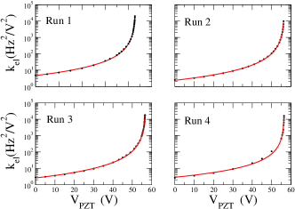
Figure 2: (Color online) Curvature coefficients data $k_{\mathrm{el}}$ versus applied voltage $V_{\mathrm{PZT}}$ and best fit with Eq. (2), but leaving the exponent as a free parameter for four different experimental runs. Given 4% uncertainty in $k_{el}$ , the reduced $\chi^{2}$ are 1.0, 0.8, 1.2, and 7.0 with the exponent left as a free parameter for Run 1, Run 2, Run 3, Run 4, respectively. Fixing the exponent to be -2 increases these values to be 16, 7.7, 6.9, and 37. The data follows a pure power law in all explored distances. The absolute distances can be assessed from the asymptotes of the curves $V^{0}_{\mathrm{PZT}}$, which are, in the progressive order of run, $43.12\pm 0.01$ V, $56.77\pm 0.02$ V, $56.99\pm 0.02$ V, and $56.66\pm 0.02$ V. The different values of $V^{0}_{\mathrm{PZT}}$ in the four runs, taken in different weeks, are due to the rearrangement of the sphere location obtained using the actuator drivers.

This is common practice in most of the Casimir force measurements in which the sensitivity of the apparatus and the zero distance are extracted from an electrostatic calibration. Depending on apparatus type, extracted quantities can be either spring constant Mohideen , torsion constant Lamoreaux ; Chan ; Decca , or effective mass like in this case Bressi ; Brown . Note that the absolute distance can be expressed in two ways: $d(V_{\mathrm{PZT}})=\beta(V_{\mathrm{PZT}}^{0}-V_{\mathrm{PZT}})$ or $d(V_{\mathrm{PZT}})=\beta{[\alpha/k_{\mathrm{el}}(V_{\mathrm{PZT}})]}^{1/2}$. Therefore, the absolute distance can be inferred either from the asymptotic limit $V^{0}_{\mathrm{PZT}}$ of the fit function or from the calibration factor $\alpha$ of the same function, indicating an interdependency of the two physical parameters appearing in Eq. (2).

The above procedure and all subsequent analysis is inapplicable if the data fail to follow the inverse square law of Eq. (2). Surprisingly, our experimental data from four separate sequences follow a power law similar to Eq. (2), but with exponents $-1.70\pm 0.01,-1.77\pm 0.02,-1.80\pm 0.01,-1.54\pm 0.02$, far from the expected value of -2. Figure 2 shows plots of $k_{\mathrm{el}}$ as a function of $V_{\mathrm{PZT}}$, with the exponent left as a free parameter.

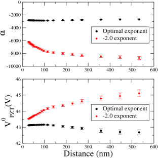
Figure 3: (Color online) Stability test of fit parameters in Eq. (2) for Run 1 with the exponent taken to be -1.7 (black, circles) and -2 (red, diamonds). Both calibration factor $\alpha$ (top plot) with units of Hz² V^-2 m^1.7 for the -1.7 exponent, and Hz² V^-2 m² for the -2.0 exponent, and the zero distance bias $V^{0}_{\mathrm{PZT}}$ (bottom plot) remain stable within 3% in the flat region at the closest separation for the exponent -1.7, while a large spreading in the two parameters is evident for the exponent -2. Note also the correlation between the fit parameters reflecting their interdependency as discussed in the text.

With the apparatus stationary, we observe a random measurement uncertainty of 4% in $k_{el}$ superimposed on a long time scale (comparable to the duration of one data run) drift, which may be due to a systematic, thermally induced change in gap size up to $\pm 200$ nm. Given the 4% error, the reduced $\chi^{2}$ is near one when the exponent is fit in the -1.7 to -1.8 range compared to around 10 for fixed -2.0 exponent. Adherence of our data to a strict power law from the farthest to the closest approach in all four cases implies the drift was not severe during our data runs, except possibly in the case of Run 4. To check the stability of the electrostatic result ruled by the unexpected power law, the following test has been conducted. We repeat fitting the data, $k_{\mathrm{el}}$ versus $V_{\mathrm{PZT}}$, starting with few points at the largest distances and by progressively including the data point corresponding to the closer distances. In this way the intrinsic instability of the fit will manifest itself through a systematic variation in the fit parameters subject to a choice of data points included. Fig. 3 shows the result of the stability test for Run 1.

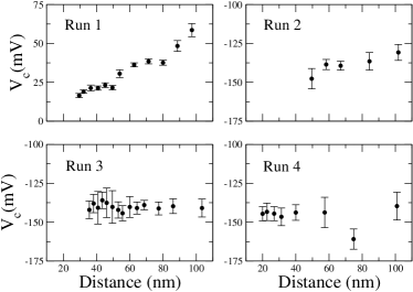
Figure 4: Dependence of the contact potential versus sphere-plane separation. Two noticeable behaviors are a linear dependence on the separation (Run 1 and Run 2) and a settlement to a constant contact potential at the smallest explored distances (Run 3 and Run 4). In Run 1 the uppermost point of the sphere is different from the other, successive three runs as the latter were taken after having tilted the sphere by 0.05 radians, to check the sensitivity to local surface details. Note that in Run 1, $V_{c}$ is positive while it is negative and converges to $V_{c}\simeq$ -150 mV at the smallest separations for other runs.

The electrostatic fit with the exponent of -1.7 displays a stable region at the shortest separation gap corresponding to the inclusion of most data points. Excluding data points simply makes the error bar larger, while the fit parameters remain stable. Forcing the exponent to be -2, on the other hand, leads to unsatisfactory calibration results, as the parameters start to drift immediately from the outset and do not display any stable region. More than 40% variations in both the calibration factor and the zero distance are found in this case. The instability is already present at the largest distances, indicating that the source of deviation from pure Coulombian behavior, for instance due to patch potentials, is still effective. Runs 2, 3 and 4 exhibit similar behavior. In order to further test the consistency of the electrostatic calibration, we have compared the absolute distances obtained from the two methods outlined above, getting a mutual agreement within 2 $\%$ for the fit with the -1.7 exponent at all distances, and deviations of 20 $\%$ if the fitting exponent is instead fixed to be -2.

The unexpected power law poses a significant limit on the validity of our electrostatic calibration. Here, we briefly examine some hypotheses which could potentially explain a deviation from the expected power law. Static deflection of cantilever: The spring constant of our cantilever is extremely stiff (about 5400 N/m). Using Hooke’s law, a deflection experienced by the cantilever due to an electrostatic force at 100 nm with an applied voltage of 100 mV is less than 0.2 $\AA$. Hence, the static deflection should play little role. Thermal drift: Even though the temperature of the cantilever is actively stabilized by a Peltier cooler, the rest of the system is still subject to global thermal variation. In order to see this, we have measured $k_{\mathrm{el}}$ with respect to time at a nominally fixed distance. In the worst circumstance, the gap separation during the course of measurements can drift as much as 200 nm in either direction. Although such a drift could in principle affect the inferred exponent, a highly unlikely non-linear monotonic drift would be necessary to account for the consistently observed anomaly in each independent run. Non-linearity of the PZT translation: The linearity of the PZT translation has been tested under a number of different circumstances. Notice that the translation intervals between the data points in each of the runs shown in Fig. 2 are completely random. Yet, all of the runs obey a specific power law in all distances. The PZT was also independently calibrated by fiber optic interferometer with a consistent, linear actuation coefficient factor $\beta=87\pm 2$ nm/V. Non-linear oscillation of cantilever: The cantilever is driven at resonance in a phase-locked loop, a routine technique adopted by many groups Decca ; Albrecht ; Jourdan ; Giessbl . Higher order terms in the force expansion should produce higher harmonics of the drive frequency. Then the assumption that the frequency shift is simply proportional to the gradient of the external force $F^{\prime}(d)$ could lead to erroneous assessments of $k_{\mathrm{el}}$, eventually affecting the exponent. We have not observed higher harmonics in the frequency spectrum of the resonator. Surface roughness: The deviation from geometrical ideality and its influence on the local capacitances Boyer could in principle play a role especially at the smallest distances. However with the measured rms values of roughness for the two surfaces we find the corrections negligible, as we discuss in detail elsewhere Kimthesis .

After discarding the hypotheses above, we may consider the effect of the patch surface potentials. Patch effects are expected to induce deviations from the Coulombian scaling with distance Speake , and we have found another anomaly corroborating this hypothesis. Indeed, our technique for obtaining the parabola curvatures at all distances reveals that the contact potential depends on distance, as shown in Fig. 4. In runs 1 and 2, the contact potentials appear to be distance-dependent. This finding calls for a more careful analysis of previous experiments in which the determinations of the contact potential have been performed at relatively large distances, typically above 1 $\mu$m. To see this more clearly, we evaluate the equivalent voltage $V_{\mathrm{eq}}=(\pi/d)\sqrt{\hbar c/360\epsilon_{0}}$ necessary to mimic the Casimir force at a given distance, as first discussed in OnoCaru . At 1 $\mu$m, the magnitude of the Casimir force is equivalent to that from an uncompensated voltage of 10 mV between the two surfaces, which should be compared to variations of 90 mV and 50 mV of the measured contact potentials in Run 1 and Run 2, respectively. The determination of the contact potential at large distances, as usually performed in various experiments, may therefore lead to a spurious signal of electrostatic origin if the contact potential at smaller distances is only partly compensated by an external counterbias.

Once the anomalous scaling exponent and the distance dependent residual voltage are taken into account, one can look for the distance dependence of $\nu_{0}^{2}$. A distant-dependent frequency should signal forces such as the Casimir force and/or forces due to surface potentials related with patch effects Speake . Disentangling forces of different origins becomes exceedingly complex with the unexpected power law found in the electrostatic analysis. Preliminary residual fitting indicate that the exponents obtained for Run 1 and Run 3 are $-2.12\pm 0.16$ and $-3.64\pm 0.25$, respectively, systematically smaller than -4 expected for the Casimir force Kimthesis .

Finally, we emphasize that the study of the Casimir force should be regarded as an extension of previous van der Waals force measurements with AFM techniques, since the underlying physics governing the short range forces between closely spaced bodies should be the same. Some of the systematic effects discussed here have been extensively discussed in the AFM literature Giessbl ; Cappella ; Garcia . Although we cannot draw substantial conclusions about the observation of the Casimir force itself from our data, the experimental procedure outlined in this report should provide an optimal strategy to handle contact potentials at all distances. Apart from looking for confirmation of the observed anomalies in other experimental setups, we believe that our findings call for a reanalysis of previous Casimir force experiments in the sphere-plane geometry, a check of the claimed accuracy, and for the systematic control of the effect of uncompensated patch potentials.

^∗Present address: Department of Physics, Yale University, 217 Prospect Street, New Haven, CT 06520-8120.

We are grateful to G. Carugno, H.B. Chan, S.K. Lamoreaux, J.N. Munday, and A. Parsegian for useful discussions. We also thank R. Johnson for technical support.

References

- (1) H.B.G. Casimir, Proc. K. Ned. Akad. Wet. B 51, 793 (1948).
- (2) P.W. Milonni, The Quantum Vacuum (Academic Press, San Diego, 1994).
- (3) M. Bordag, U. Mohideen, and V. M. Mostepanenko, Phys. Rep. 353, 1 (2001).
- (4) G. Bressi et al., Phys. Rev. Lett. 88, 041804 (2002).
- (5) S.K. Lamoreaux, Phys. Rev. Lett. 78, 5 (1997).
- (6) U. Mohideen and A. Roy, Phys. Rev. Lett. 81, 4549 (1998).
- (7) H.B. Chan et al., Science 291, 1941 (2001).
- (8) R.S. Decca et al., Phys. Rev. Lett. 91, 050402 (2003).
- (9) E. Fischbach and C. L. Talmadge, The Search for Non-Newtonian Gravity (AIP/Springer-Verlag, New York, 1999).
- (10) R. Onofrio, New J. Phys. 8, 237 (2006).
- (11) C. C. Speake and C. Trenkel, Phys. Rev. Lett. 90, 160403 (2003).
- (12) N. A. Burnham, R. J. Colton, and H. M. Pollock, Phys. Rev. Lett. 69, 144 (1992).
- (13) J. M. R. Weaver and D. W. Abraham, J. Vac. Sci. Techn. B 9, 1559 (1991).
- (14) B. D. Terris et al., Phys. Rev. Lett. 63, 2669 (1989).
- (15) G. S. Blackman, C. M. Mate, and M. R. Philpott, Phys. Rev. Lett. 65, 2270 (1990).
- (16) B. C. Stipe et al., Phys. Rev. Lett. 87, 096801 (2001).
- (17) M. Brown-Hayes et al., Phys. Rev. A 72, 052102 (2005).
- (18) D. Rugar, H. J. Marmin, and P. Guethner, Appl. Phys. Lett. 55, 2588 (1989).
- (19) T. R. Albrecht et al., J. Appl. Phys. 69, 668 (1991).
- (20) J. Blocki et al., Ann. Phys. 105, 427 (1977).
- (21) G. Jourdan et al., E-Print arXiv:0712.1767.
- (22) F. Giessibl, Rev. Mod. Phys. 75, 949 (2003).
- (23) L. Boyer et al., J. Phys. D: Appl. Phys. 27, 1504 (1994).
- (24) W. J. Kim, Towards the experimental verification of macroscopic phenomena in quantum electrodynamics, Ph. D. Thesis, Dartmouth College, August 2007; W.J. Kim et al., in preparation.
- (25) R. Onofrio and G. Carugno, Phys. Lett. A 198, 365 (1995).
- (26) B. Cappella and G. Dietler, Surf. Sci. Rep. 34, 1 (1999).
- (27) R. García and R. Pérez, Surf. Sci. Rep. 47, 197 (2002).