A Smaller Radius for the Transiting Exoplanet WASP-10b¹

Abstract

We present photometry of WASP-10 during a transit of its short–period Jovian planet. We employed the novel PSF–shaping capabilities of the OPTIC camera mounted on the UH 2.2 m telescope to achieve a photometric precision of $4.7\times 10^{-4}$ per 1.3 min sample. With this new light curve, in conjunction with stellar evolutionary models, we improve on existing measurements of the planetary, stellar and orbital parameters. We find a stellar radius $R_{\star}=0.698\pm 0.012$ $R_{\odot}$ and a planetary radius $R_{P}=1.080\pm 0.020$ $R_{\rm Jup}$. The quoted errors do not include any possible systematic errors in the stellar evolutionary models. Our measurement improves the precision of the planet’s radius by a factor of 4, and revises the previous estimate downward by 16% (2.5$\sigma$, where $\sigma$ is the quadrature sum of the respective confidence limits). Our measured radius of WASP-10b is consistent with previously published theoretical radii for irradiated Jovian planets.

1. Introduction

When an exoplanet transits its star it provides a valuable opportunity to study the physical characteristics of planets outside our solar system. Photometric survey teams are discovering a rapidly growing number of short–period planets transiting relatively bright ($9\lesssim V\lesssim 13$) Sun–like stars by monitoring the brightnesses of hundreds of thousands of stars for weeks or months, and following up on transit candidates with spectroscopy to rule out false positives (Alonso et al., 2004; McCullough et al., 2006; Bakos et al., 2007; Cameron et al., 2007; Barge et al., 2008). With this windfall of new planet discoveries comes a need for efficient and precise photometric follow–up. Measuring planet properties precisely enough for meaningful tests of theoretical models of planetary interiors requires transit light curves with good photometric precision ($<$10^-3) and high cadence ($<$1 min). In the past these requirements have often been met by combining photometry from many transit events (Holman et al., 2006; Winn et al., 2007b), or observing from space using the Hubble  and Spitzer  space telescopes (Brown et al., 2001; Gillon et al., 2007). These approaches work but they are costly in time and/or resources.

Our approach is to capitalize on the strengths of a relatively new type of detector: the orthogonal transfer array (OTA; Tonry et al., 1997). OTA detectors are charge-coupled devices (CCDs) employing a novel four–phase gate structure to allow accumulated charge to be shifted in two dimensions during an exposure. Usually, this capability is used to compensate for image motion, providing on–chip tip–tilt correction and a narrower point spread function (PSF). However, as demonstrated by Howell et al. (2003), OTAs can also be utilized to deliberately broaden PSFs in a manner that is well suited for high–precision photometry. The method of “PSF shaping” uses a raster scan to distribute the accumulated signal from each star over many pixels within a well-defined region of the detector, thereby collecting more light per exposure and increasing the observing duty cycle compared to traditional CCDs. This OTA observing mode provides benefits similar to defocusing, but without the downside of a spatially and chromatically varying PSF (Howell et al., 2003; Tonry et al., 2005).

In this Letter, we present new OTA-based photometry for a transiting planetary system recently announced by the Super Wide-Angle Search for Planets (SuperWASP) consortium. The planet, WASP-10b, is a 3.3 $M_{\rm Jup}$ planet in an eccentric, 3.09 day orbit around a $V=12.7$ K–type dwarf (Christian et al., 2008, hereafter C08). C08 measured a radius for WASP-10b that is much larger than predicted by models of planetary interiors. In § 2 we present our observations. We describe our data reduction procedures in § 3 and our light curve modeling procedure and error analysis in § 4. We present our results in § 5 and conclude in § 6 with a brief discussion of our findings.

2. Observations

Figure 1.— Example of an OPTIC PSF selected from the WASP-10 field. Throughout the exposure, the accumulated signal from the incident stellar PSF is shifted into neighboring pixels to produce a PSF confined to an approximately box–shaped region. The inset in the lower left region shows a separate, 5–second “snap-shot” exposure of WASP-10 with no OT guiding. The solid line shows the star aperture used to calculate the instrumental magnitude of the star. The background level is estimated from the mean level measured from the four flanking boxes (dashed lines).

We observed WASP-10 on UT August 16, spanning a transit time predicted by the ephemeris of C08. We used the Orthogonal Parallel Transfer Imaging Camera (OPTIC) on the University of Hawaii 2.2 m telescope atop Mauna Kea, Hawaii. OPTIC consists of two $2048\times 4096$ pixel Lincoln Lab CCID28 OTA detectors with 15 $\mu$m pixels, corresponding to 0$\farcs$135 pixel^-1 and a $9\farcm 2\times 9\farcm 2$ field of view (Howell et al., 2003). Each detector is read out through two amplifiers, dividing the frame into four quadrants. The portions of each quadrant closest to the amplifiers can be read out without disturbing the rest of the detector. Small subregions near the amplifiers can be read out rapidly (at a rate of up to 100 Hz) to monitor the position of one to four guide stars. The centroids of the guide stars are analyzed and can be used to shift charge in the science regions to compensate for image motion due to seeing and telescope guiding errors. In our application, we used a single OTA guide star as a reference point to define the origin of the shaped–PSF raster scan. We maximized our field of view by using the remaining three guide regions to image the target field.

We observed WASP-10 continuously for 4.35 hr spanning the predicted mid-transit time. Conditions were photometric. The seeing ranged from 0$\farcs$5 to 1$\farcs$2. We observed through a Sloan $z^{\prime}$ filter, the reddest broad–band filter available, to minimize the effects of differential atmospheric extinction on the relative photometry, and to minimize the effects of limb darkening on the transit light curve. We shifted the charge during each integration to form a square PSF with a side length of 20 pixels (2$\farcs$7). During each exposure, the on–chip raster scan was traced out 11 times to uniformly fill in the shaped–PSF region. An example of a WASP-10 PSF is shown in Figure 1. The integration time was 50 s, the readout time was 25 s, and the reset and setup operations took an additional 4 s. The resulting cadence was 79 seconds, corresponding to a 63% duty cycle.

3. Data Reduction

To calibrate the science images, we first subtracted the bias level corresponding to each of the four amplifiers. Visual examination of a median bias frame revealed that the bias offset is nearly constant across the detector rows. We opted to estimate the bias level of the individual science frames using the median of each 32–pixel–wide over–scan row. For flat–field calibration, we normalized individual dome flats by dividing each quadrant by the median value. We then applied a median filter to the stacked set of normalized flats to form a master flat for each night. Finally, we constructed a customized flat for each science frame by convolving the unshifted master flat with the OTA shift pattern (which is recorded in an auxiliary file at the end of each exposure) (Howell et al., 2003).

We performed aperture photometry using custom procedures written in IDL. The flux from each star was measured by summing the counts within a square aperture centered on the PSF. Before the summation, we subtracted the background level, taken to be the (outlier–rejected) mean count level among four rectangular regions flanking the star aperture. The star aperture and sky regions are illustrated in Figure 1.

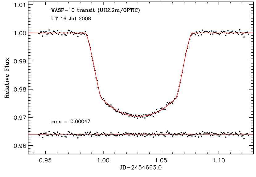
Figure 2.— Relative photometry of WASP-10. The solid red line shows the best–fitting model light curve and the residuals (O-C) are plotted belo.

Ideally, the PSF shaping procedure confines the accumulated charge for each star within a well–defined region of the detector that is common to all images. However, the telescope focus gradually drifted, resulting in variations in the full width at half maximum (FWHM) of the shaped-PSFs ranging from the nominal 20 pixels up to 24 pixels before we noticed this problem and refocused the telescope. We also noticed a faint halo surrounding the main PSF, extending to several pixels beyond the nominal PSF width. To ensure that our digital aperture captures all of the incident flux, we used a very wide aperture width of 50 pixels, chosen because it gave the smallest scatter in relative flux outside of the transit. The sky regions extend from 30 to 70 pixels from the center of the PSF.

To correct for variations in sky transparency, we divided the the flux of WASP-10 by the sum of the fluxes of 5 comparison stars with apparent magnitudes comparable to WASP-10. We used the root–mean–square (rms) scatter of the out–of–transit (OOT) points as an estimate for the individual measurement uncertainties. Our relative photometric measurements of WASP-10 are shown in Figure 2, and listed in Table 1 along with with the heliocentric Julian dates (HJD) of observation.

4. Modeling

We determined the stellar, planetary and orbital characteristics by (1) fitting the light curve with a model consisting of a star and planet in Keplerian orbit around their center of mass; (2) combining the results with stellar-evolutionary models to break the modeling degeneracies inherent in the light-curve model.

4.1. Photometric Model

Our light curve fitting procedure is similar to that of Holman et al. (2006) and Winn et al. (2007a), and uses the analytic formulas of Mandel & Agol (2002) to compute the integrated flux from the uneclipsed stellar surface as a function of the relative positions of the star and planet. The parameters were the stellar radius $R_{*}$ and mass $M_{*}$, the planetary radius $R_{P}$ and mass $M_{P}$, the orbital inclination $i$, period $P$, eccentricity $e$, argument of periastron $\omega$, and mid–transit time $T_{c}$. We fixed $P$ at the value $3.0927616$ d given by C08, which has negligible uncertainty for for our purpose. Due to the well-known fitting degeneracies $M_{p}\propto M_{\star}^{2/3}$ and $R_{p}\propto R_{\star}\propto M_{\star}^{1/3}$ (see, e.g., Winn 2008) we fixed $M_{*}$ at a fiducial value, thereby solving effectively for $R_{*}/a$ and $R_{P}/a$ rather than $R_{*}$ and $R_{P}$. The planet mass $M_{P}$ is included for completeness but the data are highly insensitive to this parameter. We measured $\omega$ and $e$ by fitting a Keplerian model to the radial velocity (RV) measurements reported by C08 and fixed the parameters in our subsequent analysis ($e=0.051$, $\omega=153$ deg). Because the eccentricity is so close to zero, we found that the actual values had very little effect on our results. There were four other free parameters: two parameters describing a linear function of airmass used to correct for differential airmass extinction, and the two coefficients in the quadratic limb darkening law. We fitted the model to our photometric observations using the goodness–of–fit statistic

$$\chi^{2}=\sum_{i}\left(\frac{f_{i}({\rm obs})-f_{i}({\rm calc})}{\sigma_{i}}\right)^{2}$$ (1)

where $f_{i}({\rm obs})$ and $f_{i}({\rm calc})$ are the observed and computed fluxes, respectively, and $\sigma_{i}$ is the uncertainty of each flux measurement, set equal to 0.000475 for our measurements, for reasons explained below.

To determine the best-fitting parameter values and their uncertainties, we used a Markov Chain Monte Carlo algorithm with a Gibbs sampler (see e.g. Winn et al., 2008b, and references therein). We created 10 chains of $10^{6}$ steps each, and combined them after verifying that the chains were converged and well-mixed. The recorded sequence of parameter combinations provides the posterior probability distribution of each parameter. We record the 15.9, 50.0, and 84.1 percentile levels in the cumulative distribution. For each parameter we quote the 50.0% level (the median) as the “best value,” and use the 84.1% and 15.9% levels to define the “one sigma” upper and lower confidence limits.

After optimizing the model parameters, we calculated the residuals to assess the photometric noise, and in particular the time-correlated noise that may arise from instrumental, atmospheric and astrophysical sources—the so–called “red noise”—using the approach outlined by Winn et al. (2008b, see also Gillon et al. 2006). We averaged the residuals into $M$ bins of $N$ points and measured the standard deviation, $\sigma_{N}$, of the binned residuals. If the noise were described by a Gaussian distribution then the rms of each grouping of residuals should decrease as $N^{-1/2}[M/(M-1)]^{1/2}~{}\sigma_{1}$, where $\sigma_{1}$ is the rms of the unbinned residuals. Correlated noise would usually cause the observed scatter to be larger than this expectation, by some factor $\beta$. We computed $\beta$ for binning intervals ranging from 5 to 20 minutes, finding $\beta\approx 1$. For this reason we set our measurement uncertainties equal to $\sigma_{1}=0.000475$ (0.5 mmag).

4.2. Stellar Evolutionary Models

To break the fitting degeneracies $M_{p}\propto M_{\star}^{2/3}$ and $R_{p}\propto R_{\star}\propto M_{\star}^{1/3}$, we required consistency between the observed properties of the star, the stellar mean density $\rho_{\star}$ that can be derived from the photometric parameter $a/R_{\star}$ (Seager & Mallen-Ornelas 2003, Sozzetti et al. 2007, Torres et al. 2008), and the Yonsei-Yale (Y²) stellar evolution models by Yi et al. (2001) and Demarque et al. (2004). The inputs were $T_{\rm eff}=4675\pm 100$ K and [Fe/H] $=0.03\pm 0.20$ from C08, and the stellar mean density $\rho_{\star}=3.099\pm 0.088$ g cm^-3 derived from the light curve. We computed isochrones for the allowed range of metallicities, and for stellar ages ranging from 0.1 to 14 Gyr. For each stellar property (mass, radius, and age), we took a weighted average of the points on each isochrone, in which the weights were proportional to $\exp(-\chi^{2}_{\star}/2)$ with

$$\chi^{2}_{\star}=\left[\frac{\Delta{\rm[Fe/H]}}{\sigma_{{\rm[Fe/H]}}}\right]^{2}+\left[\frac{\Delta T_{\rm eff}}{\sigma_{T_{\rm eff}}}\right]^{2}+\left[\frac{\Delta\rho_{\star}}{\sigma_{\rho_{\star}}}\right]^{2}.$$ (2)

Here, the $\Delta$ quantities denote the deviations between the observed and calculated values at each point. The weights were further multiplied by a factor taking into account the number density of stars along each isochrone, assuming a Salpeter mass function. It is important to keep in mind that this procedure assumes that any systematic errors in the Y² isochrones are negligible.

5. Results

Table 2 lists the parameters for the WASP-10 planetary system derived from the analysis of our new photometry. Of particular interest are the the stellar and planetary radii, $R_{*}=0.698\pm 0.012$ $R_{\odot}$ and $R_{P}=1.080\pm 0.020$ $R_{\rm Jup}$, and the mid–transit time, which is measured with a precision of 7 s. For completeness, we also list the orbit parameters determined from our independent analysis of the RV measurements of C08. Finally, we list several other quantities derived from our light curves that can be used for additional follow–up observations and modeling efforts.

Our measured planetary, stellar and orbital parameters differ significantly from the values reported previously by C08. For example, our measurement of the stellar radius is smaller by $1.9\sigma$, where $\sigma$ is quadrature sum of the respective confidence limits, and our measured orbital inclination is higher by $2.7\sigma$. As for the planetary radius, we refined the C08 value downward by $2.5\sigma$, while improving the precision from $\approx 0.08$ $R_{\rm Jup}$ to $0.02$ $R_{\rm Jup}$. The disagreement between the two results for the planetary radius can be partly attributed to different stellar radii, as well as different transit depths: $(R_{P}/R_{*})^{2}=0.02525^{+0.00024}_{-0.00028}$ from our analysis, compared to $(R_{P}/R_{*})^{2}=0.029\pm 0.001$ from C08.

We do not know the reason for these discrepancies. C08 reported four light curves: one based on the phased photometry from the 20 cm SuperWASP survey telescope, and three higher precision light curves observed with larger 1 m class telescopes. The latter three data sets were incomplete, covering ingress or egress but not both for a given transit. In our experience, complete light curves such as ours are much preferred, as they allow for more thorough checking of the noise properties and any systematic effects. C08 did not report any tests for red noise or other systematic effects, although such effects are visually evident for the Tenagara light curve and may be present in the other light curves as well. In addition, C08 did not report whether they allowed the limb-darkening parameters to vary, or held them fixed at values deemed appropriate; it has been shown by Southworth (2008) and others that holding them fixed can result in underestimated parameter errors.

6. Summary and Discussion

We have presented high–precision photometry of the K–type star WASP-10 during the transit of its close–in Jovian planet. Our analysis has improved the precision with which the planetary, orbital and stellar properties are known. From the photometry, we improved the uncertainty in the orbit inclination angle by a factor of 2.7 and the transit depth by a factor of 3.8, and we measured the transit mid-time to 7 seconds. We also measured the stellar density ($\rho_{*}$) from the transit light curve, which we used together with stellar evolution models to measure the stellar mass to a precision of 4.6%. We used the refined stellar mass to improve the precision in the planetary radius by a factor of 4. Notably, the 1.8% uncertainty in $R_{P}$ is dominated by the uncertainty in the stellar mass, rather than the photometry.

Our determination of the planetary radius represents a 16% downward revision of the value reported by C08. Those authors found that the radius of WASP-10b was much larger than predicted by even a coreless planet model. Following C08, we compared our revised radius of WASP-10b to the theoretical predictions of Fortney et al. (2007), who provide tabulated radii for planets with a range of semimajor axes, masses, ages and heavy-element core masses. For a hydrogen-helium planet with properties appropriate to WASP-10, Fortney et al. predict a radius of 1.13 $R_{\rm Jup}$ for the case of a coreless planet with an age of 4.5 Gyr. Adding 25, 50, and 100 $M_{\oplus}$ of heavy elements (nominally in the form of a solid core) decreases the radius to 1.11, 1.09 and 1.06 $R_{\rm Jup}$, respectively. The models are able to reproduce our measured radius ($R_{P}=1.08\pm 0.02$ $R_{\rm Jup}$) by including a heavy-element core with a mass ranging from 35 $M_{\oplus}$ to 95 $M_{\oplus}$.

We also compared our WASP-10b mass and radius measurements to the theoretical models of Bodenheimer et al. (2003), who predicted the radii of gas giant planets as a function of mass, age and equilibrium temperature. Assuming a planet temperature $T_{\rm eq}=T_{\rm eff}(R_{*}/a)^{1/2}=1370$ (Table 2), Bodenheimer et al. (2003) predict $R_{P}=1.11$ $R_{\rm Jup}$ for a 4.5 Gyr, solar-composition planet. The predicted radius is essentially the same whether the composition is taken to be purely solar or if a 40 $M_{\oplus}$ core of heavy elements is included. It is also fairly insensitive to the value of $T_{\rm eq}$. Thus our measured radius is only 3% ($1.5\sigma$) smaller than predicted by Bodenheimer et al. (2003).

We conclude that WASP-10b is not significantly “inflated” beyond the expectations of standard models of gas giant planets. Instead, we find that WASP-10b is among the densest exoplanets so far discovered. Its mass and radius similar to another transiting planet, HD 17156b (Winn et al. 2008c). However, WASP-10 and HD 17156 are very different host stars. Whereas HD 17156 is metal-rich ([Fe/H]$=+0.24$) and has a mass of 1.26 $M_{\odot}$, WASP-10 is a 0.75 $M_{\odot}$ K dwarf with a much lower atmospheric abundance ([M/H]$=+0.03\pm 0.2$; C08). WASP-10 stands out as one of only nine known low-mass ($M_{*}<0.8$ $M_{\odot}$) planet host stars within 200 pc, and its planet is among the most massive so far detected in this sample of low-mass stars.

We have found the OPTIC instrument to be capable of delivering single-transit photometry that is precise enough for meaningful comparisons of observed planetary properties and theoretical models. Our WASP-10 light curve has a precision of $4.7\times 10^{-4}$ per 1.3 min sample, or $6.8\times 10^{-4}$ per 1 min bin, for a $V=12.7$ star (Figure 2). This is comparable to the precision that has been reported for composite light curves, based on observations of many transits, with traditional CCD cameras. For example, Johnson et al. (2008) presented a composite $z$-band light curve for HAT-P-1 ($V=10.4$) based on observations of 8 transits, with a precision of $5.7\times 10^{-4}$ in 1 min bins. OTAs may also prove useful for the future detection and characterization of transiting Neptune–mass and “super–Earth” planets.

Table 1Relative Photometry for WASP-10

Heliocentric Julian Date	Relative Flux
2454663.94419	0.99986
2454663.94512	0.99970
2454663.94604	1.00028
2454663.94696	1.00031
2454663.94788	0.99885
…	…

Note. — The full version of this table is available in the online edition, or by request to the authors.

Table 2System Parameters of WASP-10

Parameter	Value	68.3% Confidence Interval	Comment
Transit Parameters
Mid-transit time, $T_{c}$ [HJD]	2454664.030913	$\pm 0.000082$	A
Orbital Period, $P$ [days]	3.0927616	$\pm 0.0000112$	D
Planet-to-star radius ratio, $R_{P}/R_{*}$	0.15918	$-0.00115,+0.00050$	A
Planet-star area ratio, $(R_{P}/R_{*})^{2}$	0.02525	$-0.00028,+0.00024$	A
Scaled semimajor axis, $a/R_{*}$	11.65	$-0.13,+0.09$	A
Orbit inclination, $i$ [deg]	88.49	$-0.17,+0.22$	A
Transit impact parameter, $b$	0.299	$-0.043,+0.029$	A
Transit duration [hr]	2.2271	$-0.0068,+0.0078$	A
Transit ingress or egress duration [hr]	0.3306	$-0.0075,+0.0098$	A
Other Orbital Parameters
Semimajor axis [AU]	0.03781	$-0.00047$, $+0.00067$	B
$e\cos{\omega}$	-0.0453	$\pm 0.02$	C
$e\sin{\omega}$	0.0228	$\pm 0.03$	C
Velocity semiamplitude $K_{*}$ [m s-1]	533.1	$\pm 7.5$	C
Stellar Parameters
$M_{*}$ [$M_{\odot}$]	0.75	$-0.028,+0.040$	B
$R_{*}$ [$R_{\odot}$]	0.698	$\pm 0.012$	B
$\rho_{*}$ [$\rho_{\odot}$]	3.099	$\pm 0.088$	A
$\log g_{*}$ [cgs]	4.627	$-0.0093$,$+0.0101$	B
[M/H]	0.03	$\pm 0.2$	D
$T_{\rm eff}$ [K]	4675	$\pm 100$	D
Planetary Parameters
$M_{P}$ [$M_{Jup}$]	3.15	$-0.11$, $+0.13$	B,C
$R_{P}$ [$R_{Jup}$]	1.080	$\pm 0.020$	B
Mean density, $\rho_{P}$ [$\rho_{Jup}$]	3.11	$\pm 0.20$	B,C
$\log g_{P}$ [cgs]	3.828	$\pm 0.012$	A
Equlibrium Temperature $T_{\rm eff}(R_{*}/a)^{1/2}$ [K]	1370	$\pm 50$	D

Note. — Note.—(A) Determined from the parametric fit to our light curve. (B) Based on group A parameters supplemented by the Y² stellar evolutionary models. (C) Based on our analysis of the C08 RV measurements. (D) Reproduced from C08.

References

- Alonso et al. (2004) Alonso, R., Brown, T. M., Torres, G., Latham, D. W., Sozzetti, A., Mandushev, G., Belmonte, J. A., Charbonneau, D., Deeg, H. J., Dunham, E. W., O’Donovan, F. T., & Stefanik, R. P. 2004, ApJ, 613, L153
- Bakos et al. (2007) Bakos, G. Á., Noyes, R. W., Kovács, G., Latham, D. W., Sasselov, D. D., Torres, G., Fischer, D. A., Stefanik, R. P., Sato, B., Johnson, J. A., Pál, A., Marcy, G. W., Butler, R. P., Esquerdo, G. A., Stanek, K. Z., Lázár, J., Papp, I., Sári, P., & Sipőcz, B. 2007, ApJ, 656, 552
- Barge et al. (2008) Barge, P., Baglin, A., Auvergne, M., Rauer, H., Léger, A., Schneider, J., Pont, F., Aigrain, S., Almenara, J.-M., Alonso, R., Barbieri, M., Bordé, P., Bouchy, F., Deeg, H. J., La Reza, D., Deleuil, M., Dvorak, R., Erikson, A., Fridlund, M., Gillon, M., Gondoin, P., Guillot, T., Hatzes, A., Hebrard, G., Jorda, L., Kabath, P., Lammer, H., Llebaria, A., Loeillet, B., Magain, P., Mazeh, T., Moutou, C., Ollivier, M., Pätzold, M., Queloz, D., Rouan, D., Shporer, A., & Wuchterl, G. 2008, A&A, 482, L17
- Bodenheimer et al. (2003) Bodenheimer, P., Laughlin, G., & Lin, D. N. C. 2003, ApJ, 592, 555
- Brown et al. (2001) Brown, T. M., Charbonneau, D., Gilliland, R. L., Noyes, R. W., & Burrows, A. 2001, ApJ, 552, 699
- Cameron et al. (2007) Cameron, A. C., Bouchy, F., Hébrard, G., Maxted, P., Pollacco, D., Pont, F., Skillen, I., Smalley, B., Street, R. A., West, R. G., Wilson, D. M., Aigrain, S., Christian, D. J., Clarkson, W. I., Enoch, B., Evans, A., Fitzsimmons, A., Fleenor, M., Gillon, M., Haswell, C. A., Hebb, L., Hellier, C., Hodgkin, S. T., Horne, K., Irwin, J., Kane, S. R., Keenan, F. P., Loeillet, B., Lister, T. A., Mayor, M., Moutou, C., Norton, A. J., Osborne, J., Parley, N., Queloz, D., Ryans, R., Triaud, A. H. M. J., Udry, S., & Wheatley, P. J. 2007, MNRAS, 375, 951
- Christian et al. (2008) Christian, D. J., Gibson, N. P., Simpson, E. K., Street, R. A., Skillen, I., Pollacco, D., Collier Cameron, A., Stempels, H. C., Haswell, C. A., Horne, K., Joshi, Y. C., Keenan, F. P., Anderson, D. R., Bentley, S., Bouchy, F., Clarkson, W. I., Enoch, B., Hebb, L., Hébrard, G., Hellier, C., Irwin, J., Kane, S. R., Lister, T. A., Loeillet, B., Maxted, P., Mayor, M., McDonald, I., Moutou, C., Norton, A. J., Parley, N., Pont, F., Queloz, D., Ryans, R., Smalley, B., Smith, A. M. S., Todd, I., Udry, S., West, R. G., Wheatley, P. J., & Wilson, D. M. 2008, ArXiv: 0806.1482, 806
- Fischer et al. (2005) Fischer, D. A., Laughlin, G., Butler, P., Marcy, G., Johnson, J., Henry, G., Valenti, J., Vogt, S., Ammons, M., Robinson, S., Spear, G., Strader, J., Driscoll, P., Fuller, A., Johnson, T., Manrao, E., McCarthy, C., Muñoz, M., Tah, K. L., Wright, J., Ida, S., Sato, B., Toyota, E., & Minniti, D. 2005, ApJ, 620, 481
- Fortney et al. (2007) Fortney, J. J., Marley, M. S., & Barnes, J. W. 2007, ApJ, 659, 1661
- Gillon et al. (2007) Gillon, M., Demory, B.-O., Barman, T., Bonfils, X., Mazeh, T., Pont, F., Udry, S., Mayor, M., & Queloz, D. 2007, A&A, 471, L51
- Holman et al. (2006) Holman, M. J., Winn, J. N., Latham, D. W., O’Donovan, F. T., Charbonneau, D., Bakos, G. A., Esquerdo, G. A., Hergenrother, C., Everett, M. E., & Pál, A. 2006, ApJ, 652, 1715
- Howell et al. (2003) Howell, S. B., Everett, M. E., Tonry, J. L., Pickles, A., & Dain, C. 2003, PASP, 115, 1340
- Johnson et al. (2008) Johnson, J. A., Winn, J. N., Narita, N., Enya, K., Williams, P. K. G., Marcy, G. W., Sato, B., Ohta, Y., Taruya, A., Suto, Y., Turner, E. L., Bakos, G., Butler, R. P., Vogt, S. S., Aoki, W., Tamura, M., Yamada, T., Yoshii, Y., & Hidas, M. 2008, ArXiv: 0806.1734, 806
- Mandel & Agol (2002) Mandel, K. & Agol, E. 2002, ApJ, 580, L171
- McCullough et al. (2006) McCullough, P. R., Stys, J. E., Valenti, J. A., Johns-Krull, C. M., Janes, K. A., Heasley, J. N., Bye, B. A., Dodd, C., Fleming, S. W., Pinnick, A., Bissinger, R., Gary, B. L., Howell, P. J., & Vanmunster, T. 2006, ApJ, 648, 1228
- Tonry et al. (1997) Tonry, J., Burke, B. E., & Schechter, P. L. 1997, PASP, 109, 1154
- Tonry et al. (2005) Tonry, J. L., Howell, S. B., Everett, M. E., Rodney, S. A., Willman, M., & VanOutryve, C. 2005, PASP, 117, 281
- Torres et al. (2008) Torres, G., Winn, J. N., & Holman, M. J. 2008, ApJ, 677, 1324
- Winn et al. (2007a) Winn, J. N., Holman, M. J., Bakos, G. Á., Pál, A., Johnson, J. A., Williams, P. K. G., Shporer, A., Mazeh, T., Fernandez, J., Latham, D. W., & Gillon, M. 2007a, AJ, 134, 1707
- Winn et al. (2007b) Winn, J. N., Holman, M. J., & Roussanova, A. 2007b, ApJ, 657, 1098
- Winn (2008) Winn, J. N. 2008, arXiv:0807.4929
- Winn et al. (2008b) Winn, J. N., Holman, M. J., Torres, G., McCullough, P., Johns-Krull, C. M., Latham, D. W., Shporer, A., Mazeh, T., Garcia-Melendo, E., Foote, C., Esquerdo, G., & Everett, M. 2008b, ArXiv:0804.4475, 804