Autocatalytic reaction-diffusion processes in restricted geometries

Abstract

We study the dynamics of a system made up of particles of two different species undergoing irreversible quadratic autocatalytic reactions: $A+B\rightarrow 2A$. We especially focus on the reaction velocity and on the average time at which the system achieves its inert state. By means of both analytical and numerical methods, we are also able to highlight the role of topology in the temporal evolution of the system.

I Introduction

The interest in systems undergoing reaction-diffusion processes is experiencing a rapid growth, due to their intrinsic relevance in an extraordinary broad range of fields [1].

In particular, a great deal of experimental and theoretical work has been devoted to the study of reaction-diffusion processes embedded in restricted geometries. This expression refers to two, possibly concurrent, situations: $i.$ low dimensionality and ii. small spatial extent.

In the first case, the spectral dimension $\tilde{d}$ characterizing the diffusive behaviour of the reactants on the substrate is low $(1<\tilde{d}<2)$, and the substrate underlying the diffusion-reaction lacks spatial homogeneity. This situation is able to model media whose properties are not translationally invariant and where the reactants perform a “compact exploration” [2]. These kinds of structures can lead to a chemical behaviour significantly different from those occurring on substrates displaying a homogeneous spatial arrangement. Indeed, while in high dimensions a mean-field approach (based on classical rate equations) provides a good description, in low dimension local fluctuations are responsible for significant deviation from mean-field predictions [3].

There also exists a variety of experimental situations in which reaction-diffusion processes occur on spatial scales too small to allow an infinite volume treatment: in this case finite-size corrections to the asymptotic (infinite-volume) behaviour become predominant.

Here, differently from previous works, we explicitly examine finite size systems, i.e. no thermodynamic limit is taken [4-6]. All the quantities we calculate are hence finite, and we seek their dependence on the finite parameters of the system (volume of the substrate and concentration of the reactants). In particular, we study the dynamics of a system made up of two species particles undergoing irreversible quadratic autocatalytic reactions $A+B\rightarrow 2A$. All particles move randomly and react upon encounter with probability $1$, i.e. the reaction is strictly local and deterministic. Notice that, allowing all the particles to diffuse makes the problem under study a genuine multiparticle-diffusion problem. The latter is generally quite difficult to manage due to the fact that the effects of each single particle do not combine linearly, even in the non-interacting case. For this reason the analytic treatment often relies on simplifying assumptions which, nevertheless, preserve the main generic features of the problem. In the past, autocatalytic reactions have been extensively analyzed on Euclidean structures [7], within a continuous picture attained by the Fisher equation [8,9] which describes the system in terms of front propagation. Evidently, this picture is not suitable for low-density systems, where front propagation cannot be defined. In order to describe also the high-dilution regime, here a different approach is introduced which, as we will see, works as well for inhomogeneous structures. This way, we are also able to highlight the role of topology in the temporal evolution of the system.

In the following, we shall examine the concentration $\rho_{A}(t)$ of $A$ particles present in the system at time $t$ and its fluctuations; from $\rho_{A}(t)$ it is then possible to derive an estimate for the reaction velocity. Furthermore, we consider the average time $\tau$ (also called “Final Time”) at which the system achieves its inert state, i.e. $N_{A}=N$. As we will show, $\tau$ depends on the number of particles $N$ and on the volume $V$ of the underlying structure. More precisely, for small concentrations of the reactants, we find, both numerically and analytically, that the $\tau$ factorizes into two terms depending on $N$ and $V$, respectively.

One of the most interesting applications of the Final Time is analytic [10,11]: as we show, $\tau$ sensitively depends on the initial amount of reactant $N$ and, on low dimensional substrates $(d<2)$, by reducing the dimension $d$, the sensitivity can be further improved.

II The model

We consider a system made up of $N$ particles of two different chemical species $A$ and $B$, diffusing and reacting on a discrete substrate with no excluded volume effects. At time $t$, $N_{A}(t)$ and $N_{B}(t)$ represent the number of $A$ and $B$ particles, respectively, with $N=N_{A}+N_{B}$. Being $V$ the substrate volume, we define $\rho_{A}(t)=N_{A}(t)/V$ and $\rho_{B}(t)=N_{B}(t)/V$ as the concentrations of the two species at time $t$.

Different species particles residing at time step $t$, on the same node or on nearest-neighbour nodes react according to the mechanism $A+B\rightarrow 2A$ with reaction probability set equal to one. Notice that the previous scheme also includes possible additional products (other than $2A$) made up of some inert species of no consequences to the overall kinetics. The initial condition at time $t=0$ is $N_{A}(0)=1$ (the Source), $N_{B}(0)=N-1$, with all particles distributed randomly throughout the substrate. As a consequence of the chemical reaction defined above, $N_{A}(t)$ is a monotonic function of $t$ and, due to the finiteness of the system, it finally reaches value $N$; at that stage the system is chemically inert. The average time at which $N_{A}(t)=N$ is called “Final Time” and denoted by $\tau$.

The Final Time $\tau$ is of great experimental importance since it represents the average time when the system is inert and therefore it provides an estimate of the time when reaction-induced effects (such as side-reactions or photoemission) vanish [12]. In this perspective, deviations from the theoretical prediction of $\tau$ are, as well, noteworthy: they could reveal the existence of competitive reactions or explain how the process is affected by external radiation.

Finally, notice that the autocatalytic reaction can also be used as a model for spreading phenomena: $A(B)$ particles may stand for (irreversibly) sick (healthy) or informed (unaware) agents, respectively. For these systems a knowledge of the infection rate or information diffusion is of great importance [4,5].

III Average Final Time

As previously said, $\tau$ generally depends on the total number of agents $N$ and on the size of the lattice $V$, while its functional form is affected by the topology of the lattice itself. The analytical treatment is carried out in the two limit regimes of high and low density.

III.1 High-density regime

When $\rho=N/V\gg 1$, the substrate topology does not qualitatively affects results. We can assume that the set of $A$ particles covers a connected region of the substrate whose volume expands with a constant velocity (depending on the density $\rho$ and dimension $d$). In this case (and exactly in the limit $\rho\to\infty)$ the process can be described as the deterministic propagation of a wave front decoupled from the random motion of the agents. If we suppose the Source to be at the center of the lattice at time $t=0$, at each instant the wave front is the locus of points whose chemical distance from the center is $2t+1$. The connected region spanned by the wave front is entirely occupied by $A$ particles, while $B$ particles fill the remaining of the lattice. In particular, for a $d$-dimensional regular substrate, the region where $A$ particles concentrate is a $d$-dimensional polyhedron [4,5].

In general, for a finite system, the average Final Time is $\tau=l_{\mathrm{{max}}}/2$, where $l_{\mathrm{max}}$ is the chemical distance of the most distant point on the lattice, starting from the Source. On Euclidean geometries this yields $\tau=L/4$ for d=1 and $\tau=L/2$ for $d\geq 2$. On the other hand, on inhomogeneous structures, the dependence on $L$ is not so simple, since it involves taking the average with respect to all possible starting points for the Source.

III.2 Low-density regime

In the case of low density $(\rho\ll 1)$ the time an $A$ particle walks before meeting a $B$ particle becomes very large, so that the process is diffusion-limited. We adopt a mean-field-like approximation by assuming that the time elapsing between a reaction and the successive one is long enough that the spatial distribution of reactants can be considered random. In other words, the particles between each event have the time to redistribute randomly on the lattice and we neglect correlations between their spatial positions. Another consequence of the low concentration of reactants, is that we can just focus on two-body interactions since the event of three or more particles interacting together is unlikely. Notice that the high-dilution assumption, by itself, generally does not allow to apply the classical rate equations: when diffusion is involved also the substrate topology has to be taken into account. For this reason, in the following we will treat high and low dimensional structures separately.

High-dimensional structures $(\tilde{d}>2)$ Let us consider a given configuration of the system where $N_{A}$ and $N_{B}$ particles are present. The probability for a given B particle to encounter and react with any A particle is just the trapping probability $P_{trap}(\rho_{A},t)$ for a particle, out of $N_{B}$, in the presence of $N_{A}$ traps, both species diffusing. Under the assumptions specified above, for high-dimensional substrates [1]:

$$P_{\mathrm{{trap}}}(\rho_{A},t)=\lambda_{d}\;\rho_{A}e^{-\lambda_{d}\rho_{A}t},$$ (1)

where $\lambda_{d}$ is a constant depending on the given substrate. Form the previous equation we can calculate the average trapping time for a B particle as $\tau_{\mathrm{{trap}}}(\rho_{A})\;\sim\;\rho_{A}^{-1}$.

Let us now introduce an early-time $(t<\tau_{\mathrm{{trap}}}(\rho_{A}))$ approximation for the trapping probability: $P_{\mathrm{{trap}}}(\rho_{A},t)\sim pN_{A}$, where $p\sim V^{-1}$ is the probability that, after each reaction, two given particles first encounter at a given time (in general, this probability depends not only on the volume of the underlying structure, but also on the history of the system). This simple form for $P_{\mathrm{{trap}}}(\rho_{A},t)$ allows us to go on straightforwardly. In fact, the process can be meant as an absorbing Markov chain, with $N$ states (labeled with the total number of $A$ particles: $1,2,...,N$), and one absorbing state $(N_{A}=N)$; the chain starts from state 1. The transition matrix $\mathbf{P}$ can be written: the transition probability from a state $k$ to a state $m$ as a function of N and p is:

$$P_{k,m}={N-k\choose m-k}\left[1-(1-p)^{k}\right]^{m-k}\left[(1-p)^{k}\right]^{N-m}$$ (2)

for any $N$ and $p$. From $\mathbf{P}$ we can take the submatrix $\mathbf{Q}$, obtained subtracting the last row and column (those pertaining to the absorbing state), and compute the fundamental matrix $\mathbf{F}=(1-\mathbf{Q})^{-1}$. Now, by expanding to first order in $p$, a direct calculation shows that $\mathbf{F}$ is an upper triangular matrix given by

$$F_{k,m}=\left\{\begin{array}[]{cl}\frac{1}{m\left({N-m}\right)p}&k\geq m\\ 0&k<m.\end{array}\right.$$ (3)

The mean time $\tau$ required to reach the absorbing state N, starting from state 1 is given by the sum of the first row of $\mathbf{F}$:

$$\tau\left({N,V}\right)=\frac{1}{p}\sum\limits_{m=1}^{N-1}{\frac{1}{m(N-m)}\mathrel{\mathop{\kern 0.0pt\longrightarrow}\limits_{N\to\infty}}\frac{V\left({\gamma+\log N}\right)}{N}}$$ (4)

where $\gamma=0.577...$ is the Euler-Mascheroni constant. The last result is in perfect agreement with numerical simulations and also emphasizes $\tau$ factorization.

Low-dimensional structures $(\tilde{d}\leq 2)$. For low dimensional structures the dependence on $N$ found above is not correct. The reason is that a non-linear cooperative behaviour among particles emerges.

Let us define $\langle t_{n}\rangle$ as the average time elapsing between the $(n-1)$-th first encounter among different particles and the $n$-th one. This time just corresponds to the average time during which there are just $N_{A}(t)=n$ particles in the system. In our approximation $\langle t_{n}\rangle$ is proportional to the trapping time $\tau_{\mathrm{{trap}}}(n/V)$ in the presence of n mobile traps diffusing throughout a volume $V$ [6]. For compact exploration of the space $(\tilde{d}<2)$, $\tau_{\mathrm{{trap}}}(n/V)\sim(V/n)^{2/\tilde{d}}$. This result was derived for infinite lattices, nonetheless, it provides a good approximation also for finite lattices, provided that the time to encounter is not too large. From $\tau_{\mathrm{{trap}}}$ we obtain $\langle t_{n}\rangle$ as the average trapping time of the first out of $N-n\equiv N_{B}$ particles, that, for rare events, is just

$$\langle{t_{n}}\rangle=V^{2/\tilde{d}}\frac{n^{-2/\tilde{d}}}{N-n},$$ (5)

with logarithmic corrections in the case $\tilde{d}=2$. The time $\tau$ can therefore be written as a sum over $n$ $(n=1,2,\ldots,N-1)$ of $\langle t_{n}\rangle$. Now, by adopting a continuous approximation, we obtain for $\tilde{d}<2$ [6]:

$$\tau(N,V)\approx V^{2/\tilde{d}}\left[{\frac{\tilde{d}}{(2-\tilde{d})N}+N^{-2/\tilde{d}}\left({\log N+H_{2/\tilde{d}}}\right)+O(N^{-1})}\right],$$ (6)

where $H_{m}$ is the harmonic number. In particular, the leading-order contribution for a one-dimensional system $(\tilde{d}=d=1)$ is

$$\tau(N,V)\approx\frac{V^{2}}{N}.$$ (7)

For a two-dimensional lattice $(\tilde{d}=d=2)$

$$\tau(N,V)\approx V\log V\frac{\log N+\gamma}{N}.$$ (8)

Notice that the factorization in Eq.(6) is consistent with Eq.(4): in both cases, the factor containing the dependence on $V$ represents the average time for two particles to meet.

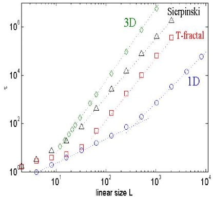
Figure 1: Scaling of $\tau$ with the linear size of the system for a one-dimensional chain (blue circles), a Sierpinski gasket (black triangles), a T-fractal (red squares), and a three-dimensional cubic lattice (green diamonds) on a double-logarithmic scale. The number of reactants is fixed at $N=1024$ for all systems. The spectral dimension for the Sierpinski and the T-graph is $\tilde{d}\approx$1.365 and $\tilde{d}\approx 1.226$, respectively. Dotted lines highlight the low-concentration regime $(L\gg 1)$, corresponding to a power law for all systems. For the one-dimensional chain, the linear high-concentration regime is also pointed up.

As can be evinced from Fig. 2, for small densities all the data collapse; moreover, in that region, the fit coefficients introduced are in good agreement with theoretical predictions.

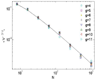
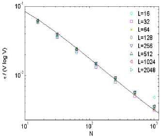
Figure 2: Rescaled Final time versus number of particles $N$ for the Sierpinski gasket (left) and the two-dimensional lattice (right). Different symbols and colours distinguish different sizes, as explained by the legend. The line provides the best fit in very good agreement with Eqs. (6) and (8), apart from sub-leading corrections in the (marginal) case $d=2$.

For low densities, the standard deviation $\sigma_{\tau}$ displays a dependence on $N$ and $L$ analogous to $\tau$; for high densities, $\sigma_{\tau}$ becomes vanishingly small, in fact the process becomes deterministic.

As anticipated in Section 1, experimental measures of $\tau$ are useful in monitoring trace reactants [6]. In the high-dilution regime, our results show that $\tau=f_{\tilde{d}}(N)g_{\tilde{d}}(V)$ and therefore, once the substrate size is fixed, the initial amount of reactant can be expressed as $N=f_{\tilde{d}}^{-1}(\tau/g_{\tilde{d}}(V))$.

A proper estimate of the sensitivity of this method is provided by the derivative $\partial N/\partial\tau$: the smaller the derivative and the larger the sensitivity. As can be evinced from Fig.3, which displays numerical results for $N$ and $\partial N/\partial\tau$, the smaller the concentration and the better the sensitivity of this technique. This makes such technique very suitable for the determination of ultratrace amounts of reactants, which is of great experimental importance [13]. Interestingly, $\partial N/\partial\tau$ also depends on the substrate topology: when $\tilde{d}\leq$ 2 and at fixed $V$, the sensitivity can be further improved by lowering the substrates dimension. Conversely, when $\tilde{d}>2,\partial N/\partial\tau$ ceases to depend on $\tilde{d}$.

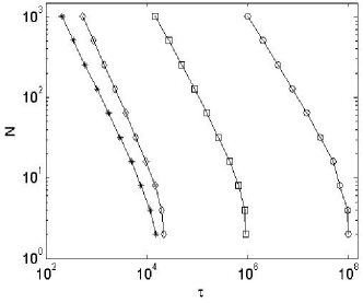
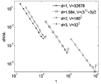
Figure 3: Log-log scale plot of the reactant amount $N$ (left panel) and its derivative $\partial N/\partial\tau$ (right panel) vs Final Time $\tau$. As shown in the legend, different substrate topologies (with approximately the same volume) are compared. Lines are guide to the eyes.

IV Temporal Evolution

In this section we deal with quantities depending explicitly on time $t$. First of all, we consider the concentration $\rho_{A}$ of $A$ particles present at time t. Due to the irreversibility of the reaction taken into account, $\rho_{A}$ is a monotonic increasing function; more precisely it is described by a sigmoidal law, typical of autocatalytic phenomena [7].

As shown in Fig.4 the curves $N_{A}(t)$ grow faster, and saturate earlier, with increasing $\tilde{d}$ ($N$ and $V$ being fixed). This is consistent with the meaning of the spectral dimension $\tilde{d}$: it describes the long-range connectivity structure of the substrate and the long-time diffusive behaviour of a random walker on the substrate. More precisely, for $\tilde{d}<2$, the number of different sites visited by each walker grows faster as $\tilde{d}$ increases, and analogously the number of meetings between walkers.

For $\tilde{d}\geq 2$ (e.g., $\tilde{d}=3$ in the figure), $N_{A}(t)$ is independent of $\tilde{d}$ and is fitted by a pure sigmoidal function. Also notice that deviations between curves relevant to different topologies are especially important at early-times, while at long times they all agree with the pure sigmoidal curve. This result is consistent with the existence of two temporal regimes concerning diffusion on low-dimensional structures [1]. As a result, the topology of the underlying structure is important only at early times, while, at long times, the system evolves as expected for high-dimensional structures.

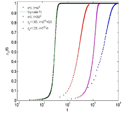
Figure 4: Normalized number of $A$ particles $N_{A}(t)/N$ vs time $t$ for a system made up of $N=128$ particles embedded on different structures, as explained in the legend. The best fit for the cubic lattice a pure sigmoidal function (see Eq. (5)), shown by the green line. The latter also provides the best fit for the long time behaviour of $N_{A}(t)/N$ on low dimensional substrates.

Within the analytic framework developed in the last section, it is possible to derive some insights into the temporal behaviour displayed by $N_{A}(t)$. Being $t(n)$ the average time at which the number of $A$ particles reaches value $n$, recalling Eq. (5) we can write

From which $N_{A}(t)=t^{-1}(N_{A})$, whose numerical solution provides an S-shaped curve consistent with data obtained from simulations.

As for transient lattices, the easy form obtained for $P_{\mathrm{trap}}(\rho_{A},t)\sim pN_{A}$ and the assumption of a uniform distribution for agents positions, allow to write a Master equation for the number of $A$ particles in the system:

$$N_{A}(t+1)=N_{A}(t)+(N-N_{A}(t))[1-(1-p)^{NA(t)}].$$ (9)

To first order in $p$: $N_{A}(t+1)=\mathcal{L}_{p}(N_{A}(t))$, being $\mathcal{L}_{p}$ a logistic-like map, with a repelling fixed point in $0$ $(f^{\prime}(0)=1+Np)$, and an attracting fixed point in $N$ $(f^{\prime}(N)=1-Np)$. Since $Np\sim\rho\ll 1$, the increment of $N_{A}(t)$ at each time step is very small (of order $p$), and we can take the evolution to be continuous. Thus we obtain

$$\rho_{A}(t)=e^{Npt}(e^{Npt}+N-1)^{-1}$$ (10)

which is in good agreement with numerical results (Fig.4).

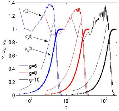
Figure 5: Reaction velocity $v$, Fluctuations $\sigma_{A}$ and concentration $\rho_{A}$ versus time for a system of $N=128$ particles diffusing on a Sierpinski gasket; three different generations (depicted in different colours) are shown. Notice $t_{v}<t_{\sigma}$.

From $\rho_{A}(t)$ one can derive the rate of reaction $v(t)=\partial_{t}N_{A}(t)$ which represents the reaction velocity. As you can see from Fig.5, in agreement with the theoretical predictions, $v(t)$ is an asymmetrical curve exhibiting a maximum at a time denoted as $t_{v,}$ obviously corresponding to a flex in $N_{A}(t)$. Interestingly, $t_{v}$ scales with the volume of the structure according to $t_{v}\sim V^{2/\tilde{d}}$ which is the same dependence shown by $\tau$. Moreover, at $t_{v}$ the population of the two species are about the same $(N_{A}(t_{v})=N_{B}(t_{v})=N/2)$.

Hence, the efficiency of the autocatalytic reaction is not constant in time but, provided the number $N$ of particles is conserved, it is maximum when the number of B particles is about $N/2$. From Eq. we can derive a similar result for the variance $\sigma_{A}(t)$ of the number of A particles present on the substrate. Interestingly, fluctuations $\sigma_{A}(t)$ peak at a time $t_{\sigma}$ which, again, depends on the system size with the same law as $\tau$; notice that $t_{\sigma}>t_{v}$.

V Conclusion

We introduced an analytic approach to deal with autocatalytic diffusion-reaction processes, also able to take into account the role played by particles discreteness and substrate topology. Within such framework, we derived in the low-density regime, for both fractal and Euclidean substrates, the exact dependence on system parameters displayed by the average Final Time, also highlighting how topology affects it. In particular, the case $d=2$ is marginal. Exact results are also found for Euclidean lattices in the limit of high density.

Theoretical results concerning the average Final Time find important applications in analytical fields, where measures of $\tau$ are exploited for detecting trace reactants. Our results suggest that the sensitivity of such technique is affected not only by the reactant concentration, but also by the topology of the structure underlying diffusion.

VI References

[1] S. Havlin, D. ben Avraham, Diffusion and Reactions in fractals and disordered systems, Cambridge University Press, Cambridge, 2000

[2] P.G. de Gennes, J. Chem. Phys. 76 3316 (1982)

[3] D. Toussaint, F. Wilczek, J. Chem. Phys. 78 2642 (1983)

[4] E. Agliari, R. Burioni, D. Cassi, F.M. Neri, Phys. Rev. E 73 046138 (2006)

[5] E. Agliari, R. Burioni, D. Cassi, F.M. Neri, Phys. Rev. E 75 021119 (2007)

[6] E. Agliari, R. Burioni, D. Cassi, F.M. Neri, Theor. Chem. Acc. (2007)

[7] J. Mai, I.M. Sokolov, A. Blumen, Europhys. Lett. 4 7 (1998)

[8] C.P. Warren, G. Mikus, E. Somfai, L.M. Sander, Phys. Rev. E 63 056103 (2001)

[9] R.A. Fisher, Ann. Eugenics 7 335 (1937), A. Kolmogorov, I. Petrovsky, P. Piskunov, Bull. Univ. Moscow. Ser. Int. Sec. A 1 1 (1937).

[10] M. Endo, S. Abe, Y. Deguchi, T. Yotsuyanagi, Talenta 47 349 (1998)

[11] M. Ishihara, M. Endo, S. Igarashi, T. Yotsuyanagi, Chem. Lett. 5 349 (1995)

[12] K. Ichimura, K. Arimitsu, M. Tahara J. Mater. Chem. 14 1164 (2004)

[13] A. Rose, Z. Zhu, C.F. Madigan, T.M. Swager, V. Bulovic Nature, 434 876 (2005); N.D. Priest, J. Environ. Monit. 6 375 (2002); J.R. McKeachie, W.R. van der Veer, L.C. Short, R.M. Garnica, M.F. Appel, T. Benter Analyst, 126 1221 (2001)