Strength and Weakness in Grover’s Quantum Search Algorithm

Abstract

Grover’s quantum search algorithm is considered as one of the milestone in the field of quantum computing. The algorithm can search for a single match in a database with $N$ records in $O(\sqrt{N})$ assuming that the item must exist in the database with quadratic speedup over the best known classical algorithm. This review paper discusses the performance of Grover’s algorithm in case of multiple matches where the problem is expected to be easier. Unfortunately, we will find that the algorithm will fail for $M>3N/4$, where $M$ is the number of matches in the list.

1 Introduction

In 1996, Lov Grover [11] presented an algorithm for searching an unstructured list of $N$ items with quadratic speed-up over classical algorithms. His original algorithm targets the case where a single match exists within the search space. Much research effort has gone into analysing and generalising his algorithm for multiple matches [3, 4, 6, 7, 8].

This paper will review the work done by others on solving the unstructured search problem on quantum computers as follows: Section 2 provides the general definition of the unstructured search problem and some of its applications. Section 3 briefly summarises the work done so far in designing algorithms concerning this problem on quantum computers. Section 4 presents Grover’s algorithm in some detail and the work done by others related to his algorithm, analysing its performance and behaviour over the range $1\leq M\leq N$ for both known and unknown number of matches $M$. The paper ends up with a general conclusion in Section 5 about Grover’s algorithm.

2 Unstructured Search Problem

Consider an unstructured list $L$ of $N$ items. For simplicity and without loss of generality we will assume that $N=2^{n}$ for some positive integer $n$. Suppose the items in the list are labelled with the integers $\{0,1,...,N-1\}$, and consider a function (oracle) $f$ which maps an item $i\in L$ to either 0 or 1 according to some properties this item should satisfy, i.e. $f:L\to\{0,1\}$. The problem is to find any $i\in L$ such that $f(i)=1$ assuming that such $i$ exists in the list. In conventional computers, solving this problem needs $O\left({N}/{M}\right)$ calls to the oracle (query), where $M$ is the number of items that satisfy the oracle.

The unstructured search problem can be considered as a general domain for a wide range of applications in computer science, for example:

• The database searching problem, where we are looking for an item in an unsorted list.

• The Boolean satisfiability problem, where we have a Boolean expression with $n$ Boolean variables and we are looking for any variable assignment that satisfies this expression.

3 Unstructured Search on Quantum Computers

Grover’s original algorithm exploits quantum parallelism by preparing a uniform superposition that represents all the items in the list then iterates both an oracle that marks the desired item by applying a phase shift of -1 on that item ($e^{\underline{i}\theta_{1}}$, with $\theta_{1}=\pi$) and nothing on the other items ($e^{\underline{i}\theta_{2}}$, with $\theta_{2}=0$) and an operator that performs inversion about the mean (diffusion operator) to amplify the amplitude of the match. The process of this operator includes the operation $\left({2\left|0\right\rangle\left\langle 0\right|-I}\right)$ which applies a phase shift of -1 on the states within the superposition ($e^{\underline{i}\phi_{1}}$, with $\phi_{1}=\pi$) except the state $\left|0\right\rangle^{\otimes n}$ where it applies nothing ($e^{\underline{i}\phi_{2}}$, with $\phi_{2}=0$) (Fig. 2) [19]. To maintain consistency with literature, this operation can also be written as $\left({I-2\left|0\right\rangle\left\langle 0\right|}\right)$ which applies a phase shift of -1 on the state $\left|0\right\rangle^{\otimes n}$ ($e^{\underline{i}\phi_{2}}$, with $\phi_{2}=\pi$) and nothing on the other states of the superposition ($e^{\underline{i}\phi_{1}}$, with $\phi_{1}=0$) together with a global phase shift of -1 (Fig. 3) [15].

It was shown that the required number of iterations is approximately ${\pi}/{4}\sqrt{N}$ which is proved to be optimal to get the highest probability with the minimum number of iterations [20], if there is exactly one match in the search space.

In [1, 10, 12, 15, 17], Grover’s algorithm is generalised by showing that the uniform superposition can be replaced by almost any arbitrary superposition and the phase shifts applied by the oracle and the diffusion operator ($e^{\underline{i}\theta_{1}},e^{\underline{i}\theta_{2}},e^{\underline{i}\phi_{1}}$ and $e^{\underline{i}\phi_{2}}$) can be generalised to deal with the arbitrary superposition and/or to increase the probability of success even with a factor increase in the number of iterations to still run in $O(\sqrt{N/M})$. These give a larger class of algorithms for amplitude amplification using variable operators from which Grover’s algorithm was shown to be a special case.

In another research direction, work has been done trying to generalise Grover’s algorithm with a uniform superposition for the case where there are a known number of multiple matches in the search space [3, 7, 8], where it was shown that the required number of iterations is approximately ${\pi}/{4}\sqrt{{N}/{M}}$ for small ${M}/{N}$. The required number of iterations will increase for $M>{N}/{2}$, i.e. the problem will be harder where it might be expected to be easier [19]. Other work has been done for a known number of multiple matches with arbitrary superposition and phase shifts [2, 4, 14, 16, 18] where the same problem for multiple matches occurs. In [4, 5, 18], a hybrid algorithm was presented to deal with this problem. It applies Grover’s fixed operators algorithm for ${\pi}/{4}\sqrt{{N}/{M}}$ times then applies one more iteration using different oracle and diffusion operator by replacing the standard phase shifts $\theta_{1}=\pi,\phi_{1}=\pi$ with accurately calculated phase shifts $\theta_{1}^{{}^{\prime}}$ and $\phi_{1}^{{}^{\prime}}$ according to the knowledge of the number of matches $M$ to get the solution with probability close to certainty. Using this algorithm will increase the hardware cost since we have to build one more oracle and one more diffusion operator for each particular $M$. For the sake of practicality, the operators should be fixed for any given $M$ and are able to handle the problem with high probability whether or not $M$ is known in advance.

In case of multiple matches, where the number of matches is unknown, an algorithm for estimating the number of matches (known as quantum counting algorithm) was presented [5, 18]. In [3], another algorithm was presented to find a match even if the number of matches is unknown which will be able to work if $M$ lies within the range $1\leq M\leq 3N/4$, otherwise it was suggested to use standard sampling techniques.

Many Grover-like algorithms for solving a wide range of applications have been presented. For example, an algorithm for the scheduling problem (intersection problem) [13] and an algorithm for minimum finding [9].

4 Grover’s Quantum Search Algorithm

4.1 Number of Matches is Known

In this section, we will present Grover’s algorithm for searching a list of size $N$ with $M$ matches such that $1\leq M\leq N$. We assume that $M$ is known in advance. For our purposes, the analysis will concentrate on the behaviour of the algorithm if iterated once, then the behaviour after $q_{G}$ iterations.

4.1.1 Iterating the Algorithm Once

Figure 1: Quantum circuit for Grover’s algorithm.

For a list of size $N=2^{n}$, the steps of the algorithm can be understood as follows (its quantum circuit is shown in Fig. 1):

• Register Preparation. Prepare a quantum register of $n+1$ qubits. The first $n$ qubits all in state $\left|0\right\rangle$ and the extra qubit in state $\left|1\right\rangle$ where it will be used as a workspace for evaluating the oracle $U_{f}$. The state of the system $\left|{W_{0}^{(G,1)}}\right\rangle$ can be written as follows, where the subscript number refers to the step within the iteration. $(G,1)$ in the superscript is the diffusion operator used in the algorithm which will be defined later and the iteration number respectively:

  $$\left|{W_{0}^{(G,1)}}\right\rangle=\left|0\right\rangle^{\otimes n}\otimes\left|1\right\rangle.$$ (1)

• Register Initialisation. Apply the Hadamard gate on each of the $n+1$ qubits in parallel so that the first $n$ qubits will contain the $2^{n}$ states representing the list and the extra qubit will be in the state ${{\left({\left|0\right\rangle-\left|1\right\rangle}\right)}\mathord{\left/{\vphantom{{\left({\left|0\right\rangle-\left|1\right\rangle}\right)}{\sqrt{2}}}}\right.\kern-1.2pt}{\sqrt{2}}}$, where $i$ is the integer representation of the items in the list:

  $$\left|{W_{1}^{(G,1)}}\right\rangle={H^{\otimes n+1}}\,\left|{W_{0}^{(G,1)}}\right\rangle={\frac{1}{\sqrt{N}}\sum\limits_{i=0}^{N-1}{\left|i\right\rangle}\otimes\left(\frac{{\left|0\right\rangle-\left|1\right\rangle}}{\sqrt{2}}\right)}.$$ (2)

• Applying the Oracle and Changing Sign. Apply the oracle $U_{f}$ that gives the amplitudes of the matches a phase shift of $-1$ ($e^{\underline{i}\pi}$), i.e. $U_{f}\left|i\right\rangle\to\left({-1}\right)^{f(i)}\left|i\right\rangle$, so that,

  $$\left|{W_{2}^{(G,1)}}\right\rangle=U_{f}\left|{W_{1}^{(G,1)}}\right\rangle=\frac{1}{{\sqrt{N}}}\sum\limits_{i=0}^{N-1}{\left|i\right\rangle\otimes\left(\frac{{\left|{0\oplus f\left(i\right)}\right\rangle-\left|{1\oplus f\left(i\right)}\right\rangle}}{\sqrt{2}}\right)}.$$ (3)

  Notice that, if $f(i)=0$, then $\left|{0\oplus f\left(i\right)}\right\rangle=\left|0\right\rangle$ and $\left|{1\oplus f\left(i\right)}\right\rangle=\left|1\right\rangle$, and if $f(i)=1$, then $\left|{0\oplus f\left(i\right)}\right\rangle=\left|1\right\rangle$ and $\left|{1\oplus f\left(i\right)}\right\rangle=\left|0\right\rangle$. Assume that $\sum\nolimits_{i}{{{}^{\prime}}}$ denotes a sum over $i$ which are desired matches and $\sum\nolimits_{i}{{{}^{\prime\prime}}}$ denotes a sum over $i$ which are undesired items in the list. So, the system $\left|{W_{2}^{(G,1)}}\right\rangle$ shown in Eqn. 3 can be re-written as follows:

  $$\left|{W_{2}^{(G,1)}}\right\rangle=\frac{1}{{\sqrt{N}}}\sum\limits_{i=0}^{N-1}{{}^{\prime\prime}\left|i\right\rangle\otimes\left(\frac{{\left|0\right\rangle-\left|1\right\rangle}}{\sqrt{2}}\right)}-\frac{1}{{\sqrt{N}}}\sum\limits_{i=0}^{N-1}{{}^{\prime}\left|i\right\rangle\otimes\left(\frac{{\left|0\right\rangle-\left|1\right\rangle}}{\sqrt{2}}\right)}.$$ (4)

  Notice the change of the sign for the states that represent the matches in the search space (phase shift of -1), with no change to the state of the extra qubit workspace, which can be removed from the system for simplicity. We end-up with a system as follows:

  $$\left|{W_{2}^{(G,1)}}\right\rangle=\frac{1}{{\sqrt{N}}}\sum\limits_{i=0}^{N-1}{{}^{\prime\prime}\left|i\right\rangle}-\frac{1}{{\sqrt{N}}}\sum\limits_{i=0}^{N-1}{{}^{\prime}\left|i\right\rangle}.$$ (5)

• Inversion about the Mean. Apply the Diffusion Operator $G$ on the first $n$ qubits. The diagonal representation of $G$ can take this form (its quantum circuit is as shown in Fig. 2 and its quantum circuit with a global phase shift factor of -1 [19] is as shown in Fig. 3):

  $$G=H^{\otimes n}\left({2\left|0\right\rangle\left\langle 0\right|-I_{n}}\right)H^{\otimes n},$$ (6)

  where the vector $\left|0\right\rangle$ used in Eqn. 6 is of length $N=2^{n}$, and $I_{n}$ is the identity matrix of size $2^{n}\times 2^{n}$. Consider a general system $\left|\psi\right\rangle$ of $n$-qubit quantum register:

  $$\left|\psi\right\rangle=\sum\limits_{j=0}^{N-1}{\alpha_{j}\left|j\right\rangle}.$$ (7)

  The effect of applying $G$ on $\left|\psi\right\rangle$ produces,

  $$G\left|\psi\right\rangle=\sum\limits_{j=0}^{N-1}{\left[{-\alpha_{j}+2\left\langle\alpha\right\rangle}\right]\left|j\right\rangle},$$ (8)

  where, $\left\langle\alpha\right\rangle=\frac{1}{N}\sum\nolimits_{j=0}^{N-1}{\alpha_{j}}$ is the mean of the amplitudes of the states in the superposition, i.e. each amplitude $\alpha_{j}$ will be transformed according to the following relation:

  $$\alpha_{j}\to\left[{-\alpha_{j}+2\left\langle\alpha\right\rangle}\right].$$ (9)

  From Eqn. 5 we can see that there are $M$ states with amplitude ${-1}/{\sqrt{N}}$ and $N-M$ states with amplitude ${1}/{\sqrt{N}}$, so the mean $\left\langle\alpha\right\rangle$ can be calculated as follows:

  $$\begin{array}[]{l}\left\langle\alpha\right\rangle=\frac{1}{N}\left({M\left({\frac{-1}{\sqrt{N}}}\right)+(N-M)\left({\frac{1}{\sqrt{N}}}\right)}\right)\\ \,\,\,\,\,\,\,\,\,\,=\frac{1}{{\sqrt{N}}}\left({1-\frac{{2M}}{N}}\right).\end{array}$$ (10)

  Figure 2: Quantum circuit for the diffusion operator $G$ over $n$ qubits.

  Figure 3: Quantum circuit for the diffusion operator $G$ over $n$ qubits with a global phase shift factor of -1 [19].

  The effect of applying $G$ on the system $\left|{W_{2}^{(G,1)}}\right\rangle$ shown in Eqn. 5 can be understood as follows:

  • The $M$ negative sign amplitudes (solutions) will be transformed from ${-1}/{\sqrt{N}}$ to $a_{1}^{G}$, where $a_{1}^{G}$ is calculated as follows: Substitute $\alpha_{j}={-1}/{\sqrt{N}}$ and $\left\langle\alpha\right\rangle$ from Eqn. 10 in Eqn. 9 we get:

    $$\begin{array}[]{l}a_{1}^{G}=-\left({\frac{-1}{\sqrt{N}}}\right)+\frac{2}{{\sqrt{N}}}\left({1-\frac{{2M}}{N}}\right)\\ \,\,\,\,\,\,\,\,=\frac{1}{\sqrt{N}}\left({3-\frac{4M}{N}}\right).\\ \end{array}$$ (11)

  • The $(N-M)$ positive sign amplitudes will be transformed from ${1}/{\sqrt{N}}$ to $b_{1}^{G}$, where $b_{1}^{G}$ is calculated as follows: Substitute $\alpha_{j}={1}/{\sqrt{N}}$ and $\left\langle\alpha\right\rangle$ from Eqn. 10 in Eqn. 9 we get:

    $$\begin{array}[]{l}b_{1}^{G}=-\left({\frac{1}{\sqrt{N}}}\right)+\frac{2}{{\sqrt{N}}}\left({1-\frac{{2M}}{N}}\right)\\ \,\,\,\,\,\,\,\,=\frac{1}{\sqrt{N}}\left({1-\frac{4M}{N}}\right).\\ \end{array}$$ (12)

  The new system $\left|{W_{3}^{(G,1)}}\right\rangle$ after applying $G$ can be written as follows, and the mechanism of amplifying the amplitudes can be understood as shown in Fig. 4:

  Figure 4: Mechanism of amplitude amplification for Grover’s algorithm with $N=8$ and $M=1$.

  $$\left|{W_{3}^{(G,1)}}\right\rangle=G\left|{W_{2}^{(G,1)}}\right\rangle=b_{1}^{G}\sum\limits_{i=0}^{N-1}{{}^{{}^{\prime\prime}}{\left|i\right\rangle}}+a_{1}^{G}\sum\limits_{i=0}^{N-1}{{}^{{}^{\prime}}{\left|i\right\rangle}},$$ (13)

  such that,

  $$M(a_{1}^{G})^{2}+(N-M)(b_{1}^{G})^{2}=1.$$ (14)

• Measurement. Measure the first $n$ qubits. The probabilities of the system will be as follows:

  • Probability $P_{s}^{\left(1\right)_{G}}$ to find a match out of the $M$ possible matches can be calculated as follows:

    $$\begin{array}[]{l}P_{s}^{\left(1\right)_{G}}=M(a_{1}^{G})^{2}\\ \,\,\,\,\,\,\,\,\,\,\,\,\,\,\,=9\left({\frac{M}{N}}\right)-24\left({\frac{M}{N}}\right)^{2}+16\left({\frac{M}{N}}\right)^{3}.\\ \end{array}$$ (15)

  • Probability $P_{ns}^{\left(1\right)_{G}}$ to find undesired result out of the states can be calculated as follows:

    $$P_{ns}^{\left(1\right)_{G}}=(N-M)(b_{1}^{G})^{2}.$$ (16)

  Notice that, using Eqn. 14,

  $$P_{s}^{\left(1\right)_{G}}+P_{ns}^{\left(1\right)_{G}}=M(a_{1}^{G})^{2}+(N-M)(b_{1}^{G})^{2}=1.\\$$ (17)

Performance of a Single Iteration

$n$, where $N=2^{n}$	Max. prob.	Min. prob.	Avg. prob.
2	1.0	0.0	0.5
3	1.0	0.0	0.5
4	1.0	0.0	0.5
5	1.0	0.0	0.5
6	1.0	0.0	0.5

Table 1: Performance of the first iteration of Grover’s algorithm with different size search space.

Considering Eqn. 11, Eqn. 12, Eqn. 13 and Eqn. 15, we can see that the probability to find a solution for a fixed size search space varies according to the number of matches $M$ in the superposition (see Fig. 5).

From Tab. 1, we can see that the maximum probability of success is always 1.0, and the minimum probability (worst case) is always 0.0. The average probability over the possible oracles for different number of matches is always 0.5. It implies that the average performance of the first iteration remains constant even with the increase of the size of the list.

To verify these results, taking into account that the oracle $U_{f}$ is taken as a black box, we can define the average probability, $average(P_{s}^{\left(1\right)_{G}})$, as follows:

$$\begin{array}[]{l}average\left(P_{s}^{\left(1\right)_{G}}\right)=\frac{1}{{2^{N}}}\sum\limits_{M=1}^{N}{{}^{N}C_{M}}P_{s}^{\left(1\right)_{G}}\\ \,\,\,\,\,\,=\frac{1}{{2^{N}}}\sum\limits_{M=1}^{N}{\frac{{N!}}{{M!\left({N-M}\right)!}}}\left({9\frac{M}{N}-24\left({\frac{M}{N}}\right)^{2}+16\left({\frac{M}{N}}\right)^{3}}\right)\\ \,\,\,\,\,\,=\frac{1}{{2^{N}}}\left({\sum\limits_{M=1}^{N}{\frac{{9\left({N-1}\right)!}}{{\left({M-1}\right)!\left({N-M}\right)!}}}-\sum\limits_{M=1}^{N}{\frac{{24\,M\,\left({N-1}\right)!}}{{N\,\left({M-1}\right)!\left({N-M}\right)!}}}+\sum\limits_{M=1}^{N}{\frac{{16\,\,M^{2}\,\,\left({N-1}\right)!}}{{N^{2}\,\,\left({M-1}\right)!\left({N-M}\right)!}}}}\right)\\ \,\,\,\,\,\,=\frac{1}{{2^{N}}}\left({9.\,2^{N-1}-24\left(\frac{{2^{N-1}+\left({N-1}\right)2^{N-2}}}{N}\right)+16\left(\frac{{3N2^{N}+N^{2}2^{N}}}{{8\,N^{2}}}\right)}\right)\\ \,\,\,\,\,\,=\frac{1}{{2^{N}}}\left({9.\,2^{N-1}-6.\,2^{N}\left(\frac{{N+1}}{N}\right)+2^{N}\left(\frac{{6N+2N^{2}}}{{N^{2}}}\right)}\right)\\ \,\,\,\,\,\,=\frac{{2^{N-1}}}{{2^{N}}}\left({9\,-12\left(\frac{{N+1}}{N}\right)+\frac{{12N+4N^{2}}}{{N^{2}}}}\right)\\ \,\,\,\,\,\,=\frac{1}{2},\\ \end{array}$$ (18)

where ${}^{N}C_{M}=\frac{{N!}}{{M!(N-M)!}}$ is the number of possible cases for $M$ matches. We can see that as the size of the list increases $(N\to\infty)$, $average(P_{s}^{\left(1\right)_{G}})$ shown in Eqn. 18 remains one-half.

Classically, we can do a single trial guess to find any match. We may succeed in finding a solution with probability $P^{(classical)}_{s}={M}/{N}$. The average probability can be calculated as follows:

$$\begin{array}[]{l}average(P_{s}^{(classical)})=\frac{1}{{2^{N}}}\sum\limits_{M=1}^{N}{{}^{N}C_{M}P_{s}^{(classical)}}\\ \,\,\,\,\,\,\,\,\,\,\,\,\,\,\,\,\,\,\,\,\,\,\,\,\,\,\,\,\,\,\,\,\,\,\,\,\,\,\,\,\,\,\,\,\,\,\,\,\,\,\,=\frac{1}{{2^{N}}}\sum\limits_{M=1}^{N}{\frac{{(N-1)!}}{{(M-1)!(N-M)!}}}\\ \,\,\,\,\,\,\,\,\,\,\,\,\,\,\,\,\,\,\,\,\,\,\,\,\,\,\,\,\,\,\,\,\,\,\,\,\,\,\,\,\,\,\,\,\,\,\,\,\,\,\,=\frac{1}{2}.\\ \end{array}$$ (19)

It means that we have an average probability one-half to find or not to find a solution by a single random guess, even with the increase in the number of matches, similar to the first iteration of Grover’s algorithm.

To compare the performance of the first iteration of Grover’s algorithm and the classical guess technique, Fig. 5 shows the probability of success of the two algorithms just mentioned as a function of $0<{M}/{N}\leq 1$.

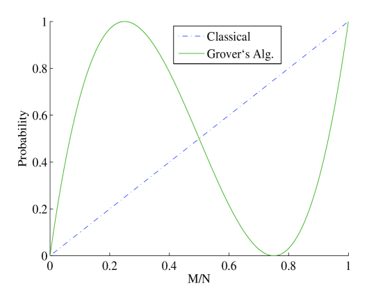
Figure 5: Probabilities of success $P_{s}^{\left(1\right)_{G}}$ and $P_{s}^{(classical)}$ as a function of ${M}/{N}$.

We can see from Fig. 5 that Grover’s algorithm solves the case where $M={N}/{4}$ with certainty. The probability of success of Grover’s algorithm will be below one-half for $M>{N}/{2}$ and will fail with certainty for $M={3N}/{4}$. The probability of success of the classical guess technique is always over that of Grover’s algorithm for $M>{N}/{2}$.

4.1.2 Iterating the Algorithm

Before we go further in the analysis of the algorithm after arbitrary number of iterations $q_{G}$, we will re-formulate the equations of the first iteration according to the way used in [3].

Initially before the first iteration, we had $M$ states with amplitude $a_{0}^{G}={1}/{\sqrt{N}}$ and $N-M$ states with amplitude $b_{0}^{G}={1}/{\sqrt{N}}$. After applying the oracle $U_{f}$ and the diffusion operator $G$, the new amplitudes $a_{1}^{G}$ and $b_{1}^{G}$ can be re-written as follows:

$$a_{1}^{G}=\frac{{N-2M}}{N}a_{0}^{G}+\frac{{2\left({N-M}\right)}}{N}b_{0}^{G},\,\,\,b_{1}^{G}=\frac{{N-2M}}{N}b_{0}^{G}-\frac{{2M}}{N}a_{0}^{G}.$$ (20)

The iterative version of the algorithm can be summarised as follows:

• Prepare a quantum register of $n+1$ qubits. The first $n$ qubits all in state $\left|0\right\rangle$ and the extra qubit in state $\left|1\right\rangle$.

• Apply the Hadamard gate on each of the $n+1$ qubits in parallel.

• Iterate the following steps $q_{G}$ times,

  • Apply the oracle $U_{f}$.

  • Apply the diffusion operator $G$ on the first $n$ qubits.

• Measure the first $n$ qubits to get the result with probability $P^{(q_{G})}_{s}$.

The system after $q_{G}\geq 1$ iterations can be written as follows,

$$\left|{W^{(G,q_{G})}}\right\rangle=b_{q}^{G}\sum\limits_{i=0}^{N-1}{{}^{{}^{\prime\prime}}{\left|i\right\rangle}}+a_{q}^{G}\sum\limits_{i=0}^{N-1}{{}^{{}^{\prime}}{\left|i\right\rangle}},$$ (21)

such that,

$$M(a_{q}^{G})^{2}+(N-M)(b_{q}^{G})^{2}=1,$$ (22)

where the amplitudes $a_{q}^{G}$ and $b_{q}^{G}$ after $q_{G}\geq 1$ iterations are defined by the following recurrence relations [3],

$$\begin{array}[]{l}a_{0}^{G}=b_{0}^{G}=\frac{1}{\sqrt{N}},\\ a_{q}^{G}=\frac{{N-2M}}{N}a_{q-1}^{G}+\frac{{2\left({N-M}\right)}}{N}b_{q-1}^{G},\,\,\,b_{q}^{G}=\frac{{N-2M}}{N}b_{q-1}^{G}-\frac{{2M}}{N}a_{q-1}^{G}.\\ \end{array}$$ (23)

Solving these recurrence relations, the closed forms can be written as follows [3]:

$$a_{q}^{G}=\frac{1}{{\sqrt{M}}}\sin\left({\left({2q_{G}+1}\right)\theta_{G}}\right),\,\,\,b_{q}^{G}=\frac{1}{{\sqrt{N-M}}}\cos\left({\left({2q_{G}+1}\right)\theta_{G}}\right),$$ (24)

where $\sin^{2}\left(\theta_{G}\right)={M}/{N}$ and $0<\theta_{G}\leq{\pi}/{2}$.

The probabilities of the system will be as follows:

• The probability of success after $q_{G}$ iterations is:

  $$P^{(q_{G})}_{s}=M\left(a_{q}^{G}\right)^{2}=\sin^{2}((2q_{G}+1)\theta_{G}).$$ (25)

• The probability of failure after $q_{G}$ iterations is:

  $$P^{(q_{G})}_{ns}=\left(N-M\right)\left(b_{q}^{G}\right)^{2}=\cos^{2}((2q_{G}+1)\theta_{G}).$$ (26)

The aim is to find a solution with probability as close as possible to certainty. It was shown in [3] that $P^{(\overline{q}_{G})}_{ns}=0$ when $\overline{q}_{G}=\left({\pi-2\theta_{G}}\right)/4\theta_{G}$, but since the number of iterations must be integer, let $q_{G}=\left\lfloor\pi/4\theta_{G}\right\rfloor$ where $\left|{q_{G}-\overline{q}_{G}}\right|\leq 1/2$. And since, $\sin^{2}\left(\theta_{G}\right)={M}/{N}$, we have for small $M/N$ that, $\theta_{G}\geq\sin\left(\theta_{G}\right)=\sqrt{{M}/{N}}$, then,

$$q_{G}=\left\lfloor{\frac{\pi}{{4\theta_{G}}}}\right\rfloor\leq{\frac{\pi}{{4\theta_{G}}}}\leq\frac{\pi}{4}\sqrt{\frac{N}{M}}=O\left({\sqrt{\frac{N}{M}}}\right),$$ (27)

where $\left\lfloor{\,\,}\right\rfloor$ is the floor operation. The lower bound of the probability of success using $q_{G}$ is $P^{(q_{G})}_{s}\geq 1-{M}/{N}\geq 0$, which is negligible only for small $M/N$.

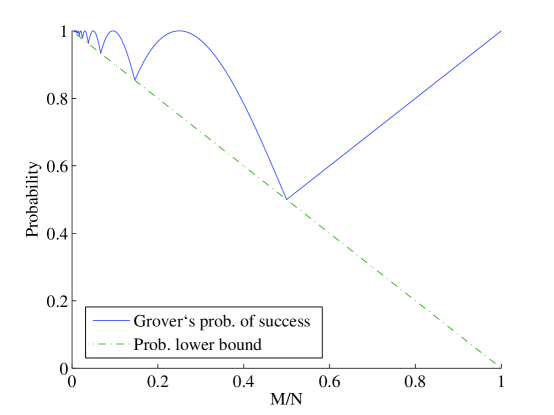
Figure 6: Probability of success of Grover’s algorithm using the required number of iterations $q_{G}$.

To demonstrate the real behaviour of Grover’s algorithm, we may plot the probability of success $P^{(q_{G})}_{s}$ using the required number of iterations $q_{G}$ for any given $M$. Fig. 6 shows this behaviour as a function of $0<{M}/{N}\leq 1$. We can see from the plot that the minimum probability that Grover’s algorithm may reach is approximately 50.0% when ${M}/{N}=0.5$. The algorithm will behave similar to the classical single random guess for ${M}/{N}>0.5$ since $q_{G}=0$ in that range. For $0.145<M/N\leq 0.5$, $q_{G}=1$ where we can see that for ${M}/{N}=0.25$ the algorithm will succeed with certainty after a single iteration. For $M/N<0.145$, $q_{G}>1$ where the algorithm will behave more reliably. In an attempt to avoid this drawback in the behaviour for multiple matches, it was proposed in [19] that we can double the search space by adding $N$ non-match items so that the number of matches will always be less than half the search space and iterate the algorithm $\pi/4\sqrt{2N/M}$ instead of $\pi/4\sqrt{N/M}$ so it still runs in $O\left({\sqrt{N/M}}\right)$. Using this approach will increase the space/time requirements to still get the result with probability at least one-half when $M=N$, where we can get the result with certainty in this case if we did not use that approach.

4.2 Number of Matches is Unknown

In case the number of matches $M$ is unknown, an algorithm that employs Grover’s algorithm [3] can be used for $1\leq M\leq{3N}/{4}$ which can be summarised as follows:

• Start with $m=1$ and $\lambda={8}/{7}$. $(\lambda$ can take any value between 1 and ${4}/{3})$

• Pick an integer $j$ between 0 and $m-1$ in a uniform random manner.

• Run $j$ iterations of Grover’s algorithm on the state: $\frac{1}{{\sqrt{N}}}\sum\limits_{i=0}^{N-1}{\left|i\right\rangle}$.

• Measure the register and assume $i$ is the output.

• If $f(i)=1$, then we found a solution and exit.

• Let $m=min\left(\lambda m,\sqrt{N}\right)$ and go to step 2.

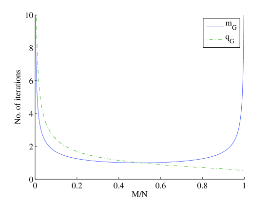
Figure 7: The actual behaviour of the functions representing the required number of iterations for known ($q_{G}=\pi/4\theta_{G}$) and unknown ($m_{G}=1/\sin\left({2\theta_{G}}\right)$) number of solutions, where the number of iterations is the flooring of the values (step function).

It was shown that the total expected number of iterations is approximately $8m_{G}\approx 4\sqrt{N/M}$ for small $M/N$ , where $m_{G}\geq 1/\sin\left({2\theta_{G}}\right)=O\left({\sqrt{N/M}}\right)$ for $M\leq{3N}/{4}$. The algorithm works only for $1\leq M\leq{3N}/{4}$, where for $M>{3N}/{4}$, a classical sampling techniques can be used.

The reason that this algorithm will fail for $M>{3N}/{4}$ is that $m_{G}$ is acting as a lower bound for $q_{G}$ for $M\leq N/2$. It handles the case where $q_{G}=0$ in a constant manner for $N/2<M\leq 3N/4$. However, it will increase exponentially for $M>{3N}/{4}$ where it is no longer able to approximate $q_{G}$, i.e. using the algorithm in that range means that the expected number of iterations will increase exponentially where the problem should be easier, as shown in Fig. 7.

5 Conclusion

In this paper, we analysed Grover’s algorithm over the whole search space. We found that, although Grover’s algorithm is optimal [20] for a single match in the search space, its reliability may decrease for multiple matches, i.e. the behaviour of the algorithm is not reliable over the whole range where the minimum probability it may reach is approximately 50.0% when ${M}/{N}=0.5$. The best behaviour is for $M/N<0.145$ and in the neighbourhood of $M/N=0.25$. The role of Grover’s algorithm disappears for ${M}/{N}>0.5$ where the required number of iterations will vanish in that range. Grover’s algorithm may not be suitable for practical implementation since a practical quantum algorithm should be able to handle both the easiest cases and the hardest cases.

References

• [1] E. Biham and D. Dan Kenigsberg. Grover’s quantum search algorithm for an arbitrary initial mixed state. Physical Review A, 66:062301, 2002.
• [2] D. Biron, O. Biham, E. Biham, M. Grassl, and D. A. Lidar. Generalized Grover search algorithm for arbitrary initial amplitude distribution. arXiv e-Print quant-ph/9801066, 1998.
• [3] M. Boyer, G. Brassard, P. Høyer, and A. Tapp. Tight bounds on quantum searching. Fortschritte der Physik, 46:493, 1998.
• [4] G. Brassard, P. Høyer, M. Mosca, , and A. Tapp. Quantum amplitude amplification and estimation. arXiv e-Print quant-ph/0005055, 2000.
• [5] G. Brassard, P. Høyer, and A. Tapp. Quantum counting. arXiv e-Print quant-ph/9805082, 1998.
• [6] G. Chen and S. Fulling. Generalization of Grover’s algorithm to multiobject search in quantum computing, part II: General unitary transformation. arXiv e-Print quant-ph/0007124, 2000.
• [7] G. Chen, S. Fulling, and J. Chen. Generalization of Grover’s algorithm to multiobject search in quantum computing, part I: Continuous time and discrete time. arXiv e-Print quant-ph/0007123, 2000.
• [8] G. Chen, S. Fulling, and M. Scully. Grover’s algorithm for multiobject search in quantum computing. arXiv e-Print quant-ph/9909040, 1999.
• [9] C. Durr and P. Høyer. A quantum algorithm for finding the minimum. arXiv e-Print quant-ph/9607014, 1996.
• [10] A. Galindo and M. A. Martin-Delgado. Family of Grover’s quantum-searching algorithms. Physical Review A, 62:062303, 2000.
• [11] L. Grover. A fast quantum mechanical algorithm for database search. In Proceedings of the 28th Annual ACM Symposium on the Theory of Computing, pages 212–219, 1996.
• [12] L. Grover. Quantum computers can search rapidly by using almost any transformation. Physical Review Letters, 80(19):4329–4332, 1998.
• [13] L. Grover. An improved quantum scheduling algorithm. arXiv e-Print quant-ph/0202033, 2002.
• [14] P. Høyer. Arbitrary phases in quantum amplitude amplification. Physical Review A, 62:052304, 2000.
• [15] R. Jozsa. Searching in Grover’s algorithm. arXiv e-Print quant-ph/9901021, 1999.
• [16] C. Li, C. Hwang, J. Hsieh, and K. Wang. A general phase matching condition for quantum searching algorithm. arXiv e-Print quant-ph/0108086, 2001.
• [17] G. L. Long. Grover algorithm with zero theoretical failure rate. arXiv e-Print quant-ph/0106071, 2001.
• [18] M. Mosca. Quantum searching, counting and amplitude amplification by eigenvector analysis. In Proceedings of Randomized Algorithms, Workshop of Mathematical Foundations of Computer Science, pages 90–100, 1998.
• [19] M. Nielsen and I. Chuang. Quantum Computation and Quantum Information. Cambridge University Press, Cambridge, United Kingdom, 2000.
• [20] C. Zalka. Grover’s quantum searching algorithm is optimal. Physical Review A, 60(4):2746–2751, 1999.