Non-commutative reading of the complex plane through Delone sequences

Abstract

The Berezin-Klauder-Toeplitz (“anti-Wick”) quantization or “non-commutative reading” of the complex plane, viewed as the phase space of a particle moving on the line, is derived from the resolution of the unity provided by the standard (or gaussian) coherent states. The construction properties of these states and their attractive properties are essentially based on the energy spectrum of the harmonic oscillator, that is on the natural numbers. This work is an attempt for following the same path by considering sequences of non-negative numbers which are not “too far” from the natural numbers. In particular, we examine the consequences of such perturbations on the non-commutative reading of the complex plane in terms of its probabilistic, functional, and localization aspects.

1 Introduction

Ever since the initial discovery of coherent states by Shrödinger in 1926 and their rediscovery in the early sixties, independently by Glauber and Sudarshan (in the context of quantum optics) and by Klauder (following a more thorough examination of the relationship between classical and quantum mechanics), many striking features and applications of these particular superpositions of harmonic oscillator eigenstates have been unveiled and explored. Certainly, one of the most intriguing and deep properties of these states is the Bayesian duality [Ali,Gazeau,Heller(2008)] that they encode between the discrete Poisson probability distribution, $n\mapsto e^{-|z|^{2}}|z|^{2}/n!$, of obtaining $n$ quantum excitations (“photons” or “quanta”) in a measurement through some counting device, and the continuous Gamma probability distribution measure $|z|^{2}\mapsto e^{-|z|^{2}}|z|^{2}/n!$ on the classical phase space, with $z$ being a parameter defining the coherent states. For this latter distribution, $|z|^{2}$ is itself a random variable, denoting the average number of photons, given that $n$ photons have been counted. Such a duality underlies the construction of all types of coherent state families, provided they satisfy a resolution of the unity condition. It turns out that this condition is equivalent to setting up a “positive operator valued measure” (POVM) on the phase space. Such a measure, in turn, leads in a natural way to a quantization procedure for the classical phase space, namely the complex plane, a procedure which we also look upon as being a “non-commutative reading” of the complex plane. (The non-commutativity is understood in the sense that we associate to each phase space point $z$ the one dimensional projection operator $\mathrm{P}_{z}$, projecting onto to the subspace generated by the coherent state vector, and then for $z\neq z^{\prime},\;\;\mathrm{P}_{z}\mathrm{P}_{z^{\prime}}\neq\mathrm{P}_{z^{\prime}}\mathrm{P}_{z}$). This “Berezin-Klauder-Töplitz” quantization turns out, in this case, to be equivalent to the canonical quantization procedure. Clearly, this non-commutative reading of the complex plane is intrinsically based on the nonnegative integers (appearing in the $n!$ term). In this paper we will follow a similar path by considering sequences of non-negative numbers which are not “too far” from the natural numbers. The resulting quantizations will then be looked upon as perturbations of the non-commutative reading given by the standard coherent states. In particular, we will examine the consequences of such perturbations on the non-commutative reading of the complex plane as they relate to their probabilistic, functional, and localization properties.

More precisely, let us consider an infinite, strictly increasing sequence of nonnegative real numbers $\{x_{n}\}_{n\in\mathbb{N}}$ such that $x_{0}=0$ and there exist $r,\;L\in\mathbb{R}$ such that $0<r\leq x_{n+1}-x_{n}\leq L<\infty$ for any $n\in\mathbb{N}$ (“Delone sequence”). To this sequence of numbers correspond the sequence of “factorials” $x_{n}!=x_{1}x_{2}\dotso x_{n}$ with $x_{0}!=1$, the “exponential”

$$\mathcal{N}(t)=\sum_{n=0}^{+\infty}\frac{t^{n}}{x_{n}!}\,,$$

the sequence of “moment” integrals,

$$x_{n}!\mu_{n}=\int_{0}^{+\infty}\frac{t^{n}}{\mathcal{N}(t)}\,dt\,.$$

and the “renormalized” sequence

$$\tilde{x}_{n}:=\frac{\mu_{n}}{\mu_{n-1}}\,x_{n}\,,\ n\geq 1\,,\quad\tilde{x}_{0}=0\,.$$

In the present study we consider various examples of such sequences, for which it is proved, analytically or numerically, that the ratios $\dfrac{\mu_{n}}{\mu_{n-1}}\to 1$.

The “non-commutative reading” of the complex plane is understood in the following sense. Standard coherent states are vectors labelled by $z\in\mathbb{C}$, $v_{z}=e^{-|z|^{2}/2}\sum_{n\in\mathbb{N}}z^{n}/\sqrt{n!}\,e_{n}$, in some separable Hilbert space with orthonormal basis $\{e_{n}\,,\,n\in\mathbb{N}\}$. One of their most striking features is that they solve the unity:

$$\mathbb{I}={\displaystyle\int\nolimits_{\mathbb{C}}}\dfrac{d^{2}z}{\pi}\,(v_{z}\,,\cdot)v_{z}\,.$$

This property allows us to transform ordinary functions $f(z)$, $z=(1/\sqrt{2})(q+ip)$, into operators $f\mapsto A_{f}={\displaystyle\int\nolimits_{\mathbb{C}}}\dfrac{d^{2}z}{\pi}\,f(z)(v_{z}\,,\cdot)v_{z}$ (“coherent state quantization”) and yields a non-commutative version of the plane illustrated by $[Q,P]=i\mathbb{I}$, where $Q\equiv A_{q}$ and $P\equiv A_{p}$. Moreover, these states minimize that non-commutativity in the sense that the uncertainty relations (or Heisenberg inequalities) for the quantized coordinates $Q$ and $P$ are saturated:

$$\Delta Q\,\Delta P=\frac{1}{2}\,,\quad\Delta Q\stackrel{{\scriptstyle\mathrm{def}}}{{=}}\sqrt{(v_{z},Q^{2}v_{z})-(v_{z},Qv_{z})^{2}}\,.$$

Such an equality produces a “fuzzy” vision of the plane with elementary “minimal” square lattice cells of side length $1/\sqrt{2}$.

Deformed coherent states are constructed using the renormalized sequence $\tilde{x}_{n}:=\mu_{n}/\mu_{n-1}\,x_{n}\,.$ $\tilde{v}_{z}=\sum_{n=0}^{\infty}1/\sqrt{\widetilde{\mathcal{N}}(|z|^{2})}\,z^{n}/\sqrt{\tilde{x}_{n}!}\,e_{n}\,.$ They also yield a resolution of the identity

$$\mathbb{I}=\int_{\mathbb{C}}\frac{\widetilde{\mathcal{N}}(|z|^{2})}{\mathcal{N}(|z|^{2})}\,\dfrac{d^{2}z}{\mu_{0}\,\pi}\,(\tilde{v}_{z}\,,\cdot)\tilde{v}_{z}\,,\ \widetilde{\mathcal{N}}(t)=\sum_{n=0}^{+\infty}\frac{t^{n}}{\tilde{x}_{n}!}\,,$$

and, by following the same procedure as above, a non-commutative version of the plane. For sequences which are perturbations of natural integers in a sense which will be made precise in the paper, the ratio $\frac{\widetilde{\mathcal{N}}(|z|^{2})}{\mu_{0}\,\mathcal{N}(|z|^{2})}$ should be $\approx 1$. This represents a mild perturbation of the standard case, with uncertainty relations modified as

$$\Delta\widetilde{Q}\,\Delta\widetilde{P}=\frac{1}{2}\,(\tilde{v}_{z},(\tilde{x}_{N+1}-\tilde{x}_{N})\tilde{v}_{z})\,,$$

where the diagonal operator $\tilde{x}_{N}$ is defined by $\tilde{x}_{N}\,e_{n}=\tilde{x}_{n}\,e_{n}$. If the differences $\tilde{x}_{n+1}-\tilde{x}_{n}$ are not too far from 1, then we deal with a kind of curved deformation of the square lattice of uncertainty cells corresponding to the standard case.

Therefore, the aim of the paper is to explain how such sequences of numbers allow one to implement a specific coherent state quantization from the complex plane, different from the canonical quantization associated with the standard integers. Accordingly, consequences in terms of phase space localization are examined.

The rest of this article is organized as follows. In Section 2, we define what we call Delone sequences of nonnegative numbers, more precisely Delone $\alpha$-perturbations of nonnegative integers, and we give a list of examples of such sequences. We revisit in Section 3 the quantization of the complex plane by using the ordinary (or Gaussian) coherent states. We then attempt in Section 4 to follow the same quantization procedure but this time based on an $\alpha$-perturbation of the natural numbers. The existence of a POVM is dependent on the associated Stieltjes moment problem according to whether the latter does or does not have an explicit solution. Even when a solution exists, it is interesting to adopt an alternative strategy for constructing a POVM which, in a certain sense, is a perturbation of the standard coherent states POVM on the complex plane. This strategy is based on a “renormalization” of the original Delone $\alpha$-perturbation of the natural numbers. We then formally proceed in Section 5 to the quantization of the complex plane arising from this renormalized sequence. We give in Section 6, some insights about the algebraic structure of the basic operators (ladder operators and the resulting successive commutators) emanating from this quantization. Next, we describe the localization aspects of the quantization of the complex plane by examining the associated orthogonal polynomials generalizing the Hermite polynomials (Section 7) and the mean values (or “lower symbols”) of operators obtained from this quantization (Section 8). Section 9 is devoted to a particularly illuminating example of $\alpha$-perturbation, namely a situation in which generalized hypergeometric functions are involved and where the probabilistic aspects of our approach are clearly brought out. In Section 10, we go back to the algebraic aspects of the quantization through $\alpha$-perturbations of natural numbers by examining the associated generalized Heisenberg algebra, a concept developed by some of us. In Section 11, we examine in a more mathematically oriented way the conditions under which it is possible to suitably Delone renormalize the $\alpha$-perturbation of the natural numbers, and we present a new result on asymptotic Poisson and Gamma distributions.

2 Delone sequences

Suppose that we are given an infinite strictly increasing sequence of nonnegative real numbers

$$\mathcal{X}=\left(x_{n}\right)_{n\in\mathbb{N}}\,,\qquad x_{0}=0\,,$$ (1)

obeying the following two constraints :

• $\mathcal{X}$ is uniformly discrete on the positive real line $\mathbb{R}^{+}\,:$ $\exists\,r>0$ such that $x_{n+1}-x_{n}\geq r$ for all $n\in N$, which means that there exists a minimal distance between two successive elements of the sequence,

• $\mathcal{X}$ is relatively dense on $\mathbb{R}^{+}\,:$ $\exists\,R>0$ such that for all $x\in\mathbb{R}^{+}$ $\exists\,n\in\mathbb{N}$ such that $|x-x_{n}|<R$, which means that there exists a maximal distance, say $L$, between two successive elements of the sequence.

These conditions imply that $\lim_{n\to\infty}x_{n}=\infty$. Actually, they mean that the sequence $\mathcal{X}$ forms a Delone set, and we will call $\mathcal{X}$ a (non-negative) Delone sequence in $\mathbb{R}^{+}$. We could choose the scale in such a way that $x_{1}=1$ or $L=1$, but we leave this as an option.

The rationale behind this set of constraints is that the sequence $\mathcal{X}$ should thus appear as not very different from the set of natural numbers. It should be noticed that from this point of view, sequences like $x_{n}=n^{\alpha}\,,\,\alpha\neq 1$, or $x_{n}=n\,\log{n}$ are not Delone. Also, familiar deformations of integers, like $q$-deformations or $(p,q)$-deformations,

$$[n]_{(p,q)}=\frac{p^{-n}-q^{n}}{p^{-1}-q}\,,\qquad[n]_{q}=[n]_{(1,q)}\,,$$ (2)

are not Delone. In this sense, these expressions could be viewed as singular deformations of the set $\mathbb{N}$.

To the sequence $\mathcal{X}$ corresponds the sequence of “factorials” $x_{n}!=x_{1}x_{2}\dotso x_{n}$ with $x_{0}!\stackrel{{\scriptstyle\mathrm{def}}}{{=}}1$, the “exponential”

$$\mathcal{N}(t)=\sum_{n=0}^{+\infty}\frac{t^{n}}{x_{n}!}\,,$$ (3)

and the sequence of “moment” integrals

$$x_{n}!\,\mu_{n}=\int_{0}^{+\infty}\frac{t^{n}}{\mathcal{N}(t)}\,dt\,,$$ (4)

in which the appearance of the “corrective” factors $\mu_{n}$’s is needed since there is no reason that the Stieltjes moment problem is solved for a generic pair $(dt/\mathcal{N}(t),x_{n}!)$, as would be the case for $(e^{-t}\,dt,n!)$.

The present study will more specifically concern sequences of numbers $\{x_{n}\}$ behaving asymptotically like natural numbers, $x_{n}\approx\mathrm{const.}\times n$ at large $n$. For convenience, we will put $\mathrm{const.}=1$ or equivalently we will consider the sequence $x_{n}/\mathrm{const.}$. We will impose more on this “natural” behavior, of course. We will require in our main example the following

Definition 2.1 (Delone perturbation of $\mathbb{N}$)

Let $\mathbb{N}\ni n\mapsto\alpha(n)$ be a bounded function with values in the interval $(-1,1)$, $\alpha(0)=0$, and such that its successive jumps $\alpha(n+1)-\alpha(n)$ have lower bound $r-1$ with $r\in(0,1)$. Then the Delone sequence

$$x_{n}=n+\alpha(n)\,,\quad n\in\mathbb{N}\,,$$ (5)

is called an $\alpha$-perturbation of the natural numbers.

Note that this $r$ is a Delone lower bound for the sequence $\{x_{n}\}_{n\in\mathbb{N}}$ in the sense of (d1).

For instance, $\alpha(n)$ could be a constant shift, $\alpha(n)=\epsilon$ for $n>0$. In order to fulfill the Delone condition (d1), we should then have $-1<\epsilon<1$ and $0<r<1$. Another simple case that will be considered in this paper is

$$0<n\mapsto\alpha(n)=\frac{an+b}{cn+d}\,,$$ (6)

with $-1<b/d<a/c<1$ or $-1<a/c<b/d<1$ and $0<r<1$.

The perturbation function could also be periodic, like

$$\alpha(n)=\epsilon\,\sin{\omega n}\,,\quad-1<\epsilon<1\,,\quad 0<r\leq 1-2|\epsilon\,\sin{\omega}|\,.$$ (7)

The function $\alpha(n)$ could even be a random perturbation.

Another interesting example is the set $\mathbb{Z}_{\beta}^{+}$ of non-negative beta-integers, i.e. all those positive real numbers which are polynomial in powers of an irrational real number $\beta>1$, when they are expanded with respect to the base $\beta$ using the usual greedy algorithm. When $\beta$ is endowed with specific properties (e.g. Pisot-Vijayaraghavan (PV) algebraic integers or more generally belonging to the so-called Parry family), these $\beta$-integers form a quasiperiodic sequence with a finite number of possible adjacent differences $x_{n+1}-x_{n}$. The number of distinct distances between consecutive $\beta$-integers is finite if and only if $\beta$ is a Parry number. It is natural to ask in case of Parry numbers, whether the corresponding $\beta$-integers behave similarly to the integers. Some answers concerning the additive, multiplicative and diffractive properties of $\beta$-integers already exist (see [Gazeau(2006)] and references therein). In view of the “quasi”-periodic distribution of the $\beta$-integers on the real line, it is pertinent to investigate the extent to which they differ from ordinary integers in an asymptotic sense, according to the nature of $\beta$.

Let us quote here precise results from [Balkova(2008)] that illustrate the similarity between sets $\mathbb{N}$ and $\mathbb{Z}^{+}_{\beta}=\{b_{n}\mid n\in\mathbb{N}\}$ for $\beta$ being a Parry number by mentioning two properties:

1. The limit $c_{\beta}:=\lim_{n\to\infty}\dfrac{b_{n}}{n}$ exists and belongs to the extension field $\mathbb{Q}(\beta)$ on the rational numbers.

2. For $\beta$ being moreover a PV number such that its minimal and its Parry polynomial coincide, the modulation $\alpha(n)=\dfrac{b_{n}}{c_{\beta}}-n$ is bounded. Parry polynomials are defined in [Balkova(2008)]

Let us mention that both of the previous asymptotic characteristics are known for $\beta$ being a quadratic Parry unit. We underline that for quadratic numbers the notions of Parry and PV numbers coincide. The following proposition providing explicit formulae for $\beta$-integers for a quadratic PV unit $\beta$ comes from [Gazeau(2006)].

Proposition 2.1

If $\beta$ is a simple quadratic PV unit, then

$${\mathbb{Z}}_{\beta}^{+}=\left\{b_{n}=c_{\beta}n+\frac{1}{\beta}\,\frac{1-\beta}{1+\beta}+\frac{\beta-1}{\beta}\,\left\{\frac{n+1}{1+\beta}\right\},\ n\in\mathbb{N}\right\},\quad\text{where}\ c_{\beta}=\dfrac{1+\beta^{2}}{\beta(1+\beta)}.$$

If $\beta$ is a non-simple quadratic PV unit, then

$${\mathbb{Z}}_{\beta}^{+}=\left\{b_{n}=c_{\beta}n+\frac{1}{\beta}\left\{\frac{n}{\beta}\right\},\ n\in\mathbb{N}\right\},\quad\text{where}\ c_{\beta}=1-\dfrac{1}{\beta^{2}}\,,$$

where $\{x\}$ denotes the fractional part of a nonnegative real number $x$.

The simplest example is provided by the set $\mathbb{Z}_{\tau}^{+}$ of non-negative $\tau$-integers, where $\beta$ is equal to the golden mean $\tau=(1+\sqrt{5})/2$. These $\tau$-integers form a quasiperiodic sequence with two possible adjacent differences $x_{n+1}-x_{n}=1$ or $1/\tau$. Their exact expression is given by

$${\mathbb{Z}}_{\tau}^{+}=\left\{b_{n}=c_{\tau}\,n-\frac{1}{\tau^{4}}+\frac{1}{\tau^{2}}\,\left\{\frac{n+1}{\tau^{2}}\right\},\ n\in\mathbb{N}\right\},\quad\text{where}\ c_{\tau}=\dfrac{1+\tau^{2}}{\tau^{3}}\approx 0.8541\,,$$

where $\{x\}$ designates the fractional part of a nonnegative real number $x$. Dividing by $c_{\tau}$ gives the “normalized” Delone sequence $x_{n}=b_{n}/c_{\tau}=n+\alpha_{\tau}(n)\,,$ with

$$\alpha_{\tau}(n)=\frac{\tau}{1+\tau^{2}}\,\left\{\frac{n+1}{\tau^{2}}\right\}-\frac{1}{\tau(1+\tau^{2})}\,.$$

Since $\{x\}\in[0,1)$, we deduce the bounds for the modulation:

$$-\frac{1}{\tau(1+\tau^{2})}\approx-0.1708<\alpha_{\tau}(n)<\frac{1}{(1+\tau^{2})}\approx 0.2764\,.$$

We will explain below how such Delone sequences of numbers allow one to implement a specific non-commutative (or “quantum”) reading of the complex plane associated to Poisson-like probability distributions and to what extent this reading is “close” to the “canonical” reading provided by natural numbers. We will start with the sequence of natural numbers and then we will generalize the procedure to sequences $\mathcal{X}$ endowed with suitable properties.

3 Natural numbers and the “fuzzy plane”

Let $\mathcal{H}$ be a separable (complex) Hilbert space with scalar product $(\cdot\,,\cdot)$ (antilinear on the left) and orthonormal basis $e_{0},e_{1},\dotsc,e_{n},\dotsc$,

$$(e_{n},e_{n^{\prime}})=\delta_{nn^{\prime}}\,.$$ (8)

To each complex number $z\in\mathbb{C}$ corresponds the following vector in $\mathcal{H}$ :

$$v_{z}=\sum_{n=0}^{\infty}e^{-\frac{|z|^{2}}{2}}\frac{z^{n}}{\sqrt{n!}}\,e_{n}\,.$$ (9)

Such a “continuous” set of vectors is called a family of standard coherent states in the quantum physics literature [Klauder,Skagerstam(1985), Ali et al(2000)]. They enjoy the following properties.

• $\|v_{z}\|=1$ (normalization).

• The map $\mathbb{C}\ni z\mapsto v_{z}$ is weakly continuous (continuity).

• The map $\mathbb{N}\in n\mapsto|(e_{n}\,,v_{z})|^{2}=e^{-|z|^{2}}\dfrac{|z|^{2n}}{n!}$ is a Poisson probability distribution with average number of successes equal to $|z|^{2}$ (discrete probabilistic content [Ali,Gazeau,Heller(2008)]).

• The map $\mathbb{C}\ni z\mapsto|(e_{n}\,,v_{z})|^{2}=e^{-|z|^{2}}\dfrac{|z|^{2n}}{n!}$ is a Gamma probability distribution (with respect to the square of the radial variable) with $n$ as a shape parameter (continuous probabilistic content [Ali,Gazeau,Heller(2008)]).

• $$\mathbb{I}={\displaystyle\int\nolimits_{\mathbb{C}}}\dfrac{d^{2}z}{\pi}\,\mathrm{P}_{z}\,,$$ (10)

  where $\mathrm{P}_{z}=(v_{z}\,,\cdot)v_{z}$ is the orthogonal projector onto the vector $v_{z}$ and the integral should be understood in the weak sense (resolution of the unity in $\mathcal{H}$).

The proof of (10) is straightforward and stems from the orthogonality of the Fourier exponentials and from the integral expression of the Gamma function which solves the moment problem for the factorial $n!$ :

$${\displaystyle\int\nolimits_{\mathbb{C}}}\dfrac{d^{2}z}{\pi}\,\mathrm{P}_{z}=\sum_{n,n^{\prime}=0}^{\infty}e_{n}\,(e_{n^{\prime}}\,,\cdot)\,\frac{1}{\sqrt{n!n^{\prime}!}}\,\int_{\mathbb{C}}\dfrac{d^{2}z}{\pi}\,e^{-|z|^{2}}z^{n}{\bar{z}}^{n^{\prime}}=\sum_{n=0}^{\infty}e_{n}\,(e_{n}\,,\cdot)=\mathbb{I}\,.$$ (11)

Property (v) is crucial in the sense that it allows one to define:

1. a normalized positive operator-valued measure (POVM) on the complex plane equipped with its Lebesgue measure $\dfrac{d^{2}z}{\pi}$ and its $\sigma-$algebra $\mathcal{F}$ of Borel sets :

   $$\mathcal{F}\ni\Delta\,\mapsto\int_{\Delta}\dfrac{d^{2}z}{\pi}\,\mathrm{P}_{z}\,\in\mathcal{L}(\mathcal{H})^{+}\,,$$ (12)

   where $\mathcal{L}(\mathcal{H})^{+}$ is the cone of positive bounded operators on $\mathcal{H}$;

2. a so-called Berezin-Klauder-Toeplitz quantization of the complex plane [Klauder(1963), Berezin(1975), Gazeau et al(2003), Klauder(1995)], which means that to a function $f(z,\bar{z})$ in the complex plane there corresponds the operator $A_{f}$ in $\mathcal{H}$ defined by

   $$f\mapsto A_{f}=\int_{\mathbb{C}}\dfrac{d^{2}z}{\pi}\,f(z,\bar{z})\mathrm{P}_{z}=\sum_{n,n^{\prime}=0}^{\infty}\left(A_{f}\right)_{nn^{\prime}}e_{n}\,(e_{n^{\prime}}\,,\cdot)\,,$$ (13)

   with matrix elements

   $$\left(A_{f}\right)_{nn^{\prime}}=\frac{1}{\sqrt{n!n^{\prime}!}}\,\int_{\mathbb{C}}\dfrac{d^{2}z}{\pi}\,f(z,\bar{z})e^{-|z|^{2}}z^{n}{\bar{z}}^{n^{\prime}}\,,$$ (14)

   provided that weak convergence holds.

We emphasize here the point that we would like the reader to understand by a non-commutative reading of the complex plane [Madore(1995)]: a non-commutative algebra of operators in $\mathcal{H}$ takes the place of the commutative algebra of complex valued functions on the plane. Note that the map (13) is linear and, in view of (10), the function $f(z,\bar{z})=1$ is mapped to the identity. These features are what we “minimally” expect from any quantization scheme.

For the simplest functions $f(z,\bar{z})=z$ and $f(z,\bar{z})=\bar{z}$ we obtain

$$A_{z} =a\,,\quad a\,e_{n}=\sqrt{n}\,e_{n-1}\,,\quad a\,e_{0}=0\,,\quad\mbox{(lowering operator)}$$ (15)

$$A_{\bar{z}} =a^{{\dagger}}\,,\quad a^{{\dagger}}\,e_{n}=\sqrt{n+1}\,e_{n+1}\quad\mbox{(raising operator)}\,.$$ (16)

These two basic operators obey the so-called canonical commutation rule : $[a,a^{{\dagger}}]=\mathbb{I}$. The number operator $N$ is defined by $N=a^{{\dagger}}a$ and is such that its spectrum is exactly $\mathbb{N}$ with eigenvectors $e_{n}$ : $Ne_{n}=ne_{n}$. The linear span of the triple $\{a,a^{{\dagger}},\mathbb{I}\}$ equipped with the operator commutator $[\cdot\,,\cdot]$ is the Weyl-Heisenberg Lie algebra, a key mathematical object for standard quantum mechanics. The fact that the complex plane has become non-commutative is apparent from the quantization of the real and imaginary parts of $z=\dfrac{1}{\sqrt{2}}(q+ip)$ :

$$A_{q}\stackrel{{\scriptstyle\mathrm{def}}}{{=}}Q=\frac{1}{\sqrt{2}}(a+a^{{\dagger}})\,,\quad A_{p}\stackrel{{\scriptstyle\mathrm{def}}}{{=}}P=\frac{1}{\sqrt{2}i}(a-a^{{\dagger}})\,,\quad[Q,P]=i\mathbb{I}\,.$$ (17)

4 Generic Delone sequences and the “fuzzy plane”

We now consider a generic Delone sequence as in (1). As a first remark, we easily assert the following result about the convergence of the associated exponential.

Proposition 4.1

Let $\mathcal{X}=\{x_{n}\}_{n\in\mathbb{N}}$ be a non-negative sequence such that $x_{n}>0$ for all $n\geq 1$ and $\lim_{n\to\infty}x_{n}=\infty$. Then its associated exponential

$$\mathcal{N}(t)=\sum_{n=0}^{+\infty}\frac{t^{n}}{x_{n}!}\,,$$ (18)

has an infinite convergence radius.

Proof.  It is enough to apply the d’Alembert criterion for a power series of the form $\sum_{n=0}^{\infty}a_{n}z^{n}$ :

$$\lim_{n\to\infty}\left|\frac{a_{n+1}}{a_{n}}\right|=\lim_{n\to\infty}\frac{1}{x_{n+1}}=0\,.$$

 

We then mimic the construction (9) by considering the following family of vectors in $\mathcal{H}$ :

$$v_{z}=\sum_{n=0}^{\infty}\frac{1}{\sqrt{\mathcal{N}(|z|^{2})}}\frac{z^{n}}{\sqrt{x_{n}!}}\,e_{n}\,.$$ (19)

These vectors still enjoy some properties similar to the standard ones.

• $\|v_{z}\|=1$ (normalization).

• The map $\mathbb{C}\ni z\mapsto v_{z}$ is weakly continuous (continuity).

• The map $\mathbb{N}\in n\mapsto|(e_{n}\,,v_{z})|^{2}=\dfrac{|z|^{2n}}{\mathcal{N}(|z|^{2})x_{n}!}$ is a Poisson-like distribution in $|z|^{2}$, with average number of successes equal to $|z|^{2}$ (discrete probabilistic content [Ali,Gazeau,Heller(2008), Bardwell,Crow(1964)]).

However, the map $\mathbb{C}\ni z\mapsto|(e_{n}\,,v_{z})|^{2}=\dfrac{|z|^{2n}}{\mathcal{N}(|z|^{2})x_{n}!}$ is not a (Gamma-like) probability distribution (with respect to the square of the radial variable in the complex plane) with $x_{n+1}$ as a shape parameter, and this is a serious setback for the Berezin-Toeplitz quantization program. Indeed there is no reason why carrying out again the calculation (13) should yield the resolution of the unity : with $\mathrm{P}_{z}=(v_{z}\,,\cdot)v_{z}$,

$$\int_{\mathbb{C}}\dfrac{d^{2}z}{\pi}\,\mathrm{P}_{z} =\sum_{n,n^{\prime}=0}^{\infty}e_{n}\,(e_{n^{\prime}}\,,\cdot)\,\frac{1}{\sqrt{x_{n}!x_{n}^{\prime}!}}\,\int_{\mathbb{C}}\dfrac{d^{2}z}{\pi}\,\frac{1}{\mathcal{N}(|z|^{2})}z^{n}{\bar{z}}^{n^{\prime}}$$

$$=\sum_{n=0}^{\infty}\frac{1}{x_{n}!}\mathcal{I}(n)e_{n}\,(e_{n}\,,\cdot)\stackrel{{\scriptstyle\mathrm{def}}}{{=}}\mathbb{F}\,$$ (20)

where $\mathbb{F}$ is a diagonal operator determined by the sequence of integrals

$$\mathcal{I}(n)=\int_{0}^{+\infty}t^{n}\,\frac{dt}{\mathcal{N}(t)}\,.$$ (21)

These integrals form a sequence of Stieltjes moments for the measure $\dfrac{dt}{\mathcal{N}(t)}$.

We are now faced with the following alternatives.

The moment problem has a solution.

More precisely, we first suppose that the Stieltjes moment problem has a solution for the sequence of factorials $\left(x_{n}!\right)_{n\in\mathbb{N}}$, i.e. there exists a probability distribution $t\mapsto w(t)$ on $[0,+\infty)$ [Ali,Gazeau,Heller(2008)] with infinite support such that

$$x_{n}!=\int_{0}^{+\infty}t^{n}\,w(t)\,dt\,.$$ (22)

We know that a necessary and sufficient condition for this is that the two matrices

$$\begin{pmatrix}1&x_{1}!&x_{2}!&\dotso&x_{n}!\\ x_{1}!&x_{2}!&x_{3}!&\dotso&x_{n+1}!\\ x_{2}!&x_{3}!&x_{4}!&\dotso&x_{n+2}!\\ \vdots&\vdots&\vdots&\ddots&\vdots\\ x_{n}!&x_{n+1}!&x_{n+2}!&\dotso&x_{2n}!\end{pmatrix}\,,\quad\begin{pmatrix}x_{1}!&x_{2}!&x_{3}!&\dotso&x_{n+1}!\\ x_{2}!&x_{3}!&x_{4}!&\dotso&x_{n+2}!\\ x_{3}!&x_{4}!&x_{5}!&\dotso&x_{n+3}!\\ \vdots&\vdots&\vdots&\ddots&\vdots\\ x_{n+1}!&x_{n+2}!&x_{n+3}!&\dotso&x_{2n+1}!\end{pmatrix}$$ (23)

have strictly positive determinants for all $n$.

Then, a natural approach is just to modify the measure in (22) by including the weight $w(|z|^{2})\,\mathcal{N}(|z|^{2})$. We then obtain the resolution of the identity :

$$\int_{\mathbb{C}}\dfrac{d^{2}z}{\pi}\,w(|z|^{2})\,\mathcal{N}(|z|^{2})\,\mathrm{P}_{z} =\sum_{n,n^{\prime}=0}^{\infty}e_{n}\,(e_{n^{\prime}}\,,\cdot)\,\frac{1}{\sqrt{x_{n}!x_{n}^{\prime}!}}\,\int_{\mathbb{C}}\dfrac{d^{2}z}{\pi}\,w(|z|^{2})\,z^{n}{\bar{z}}^{n^{\prime}}$$

$$=\sum_{n=0}^{\infty}\frac{1}{x_{n}!}\,\int_{0}^{+\infty}t^{n}\,w(t)\,dt\,e_{n}\,(e_{n}\,,\cdot)=\mathbb{I}\,.$$ (24)

Of course, in many (if not most) cases the explicit form of the measure is not known. So, at this stage, the construction of CS may remain at a formal level and we will rather adopt the approach described below.

The moment problem has no solution or has a solution with unsolved measure.

Here we will suppose that the sequence of ratios

$$\mu_{n}\stackrel{{\scriptstyle\mbox{def}}}{{=}}\frac{\mathcal{I}(n)}{x_{n}!}$$ (25)

has a finite limit as $n\to\infty$,

$$\mu_{n}\to\mu_{\infty}<\infty\,\Leftrightarrow\,\lim_{n\to\infty}\frac{\mu_{n}}{\mu_{n-1}}=1\,.$$ (26)

It is then natural to “renormalize” the non-negative Delone sequence (1) as follows.

$$\tilde{x}_{n}\stackrel{{\scriptstyle\mbox{def}}}{{=}}\frac{\mu_{n}}{\mu_{n-1}}\,x_{n}\,,\quad n\geq 1\,,\quad\tilde{x}_{0}=0\,,$$ (27)

and this entails

$$\tilde{x}_{n}!=\frac{\mu_{n}}{\mu_{0}}\,(x_{n}!)\,,\quad n\in\mathbb{N}\,.$$ (28)

The assumption (26) ensures that this renormalized sequence gets closer and closer to the original sequence, and the condition of the terms being strictly increasing is fulfilled beyond a certain point $n_{0}$. If some crossing happens for the first few elements of the sequence, we will reorder the sequence (27) so that it becomes strictly increasing; however, in order to avoid an inflation of notations, we shall maintain the same notation (possibly at the expense of some notational abuse).

We then start again the construction in (9) by considering this time the renormalized family of vectors in $\mathcal{H}$ :

$$\tilde{v}_{z}=\sum_{n=0}^{\infty}\frac{1}{\sqrt{\widetilde{\mathcal{N}}(|z|^{2})}}\frac{z^{n}}{\sqrt{\tilde{x}_{n}!}}\,e_{n}\,,$$ (29)

where $\widetilde{\mathcal{N}}(t)$ is the exponential associated to the new sequence,

$$\widetilde{\mathcal{N}}(t)=\sum_{n=0}^{+\infty}\frac{t^{n}}{\tilde{x}_{n}!}\,.$$ (30)

From (26) it is clear that this series also has an infinite radius of convergence. Now, not only do the vectors (29) enjoy properties similar to the vectors (19),

• $\|\tilde{v}_{z}\|=1$ (normalization).

• The map $\mathbb{C}\ni z\mapsto\tilde{v}_{z}$ is continuous (continuity).

• The map $\mathbb{N}\in n\mapsto|(e_{n}\,,\tilde{v}_{z})|^{2}=\dfrac{|z|^{2n}}{\widetilde{\mathcal{N}}(|z|^{2})\tilde{x}_{n}!}$ is a Poisson-like distribution with average number of occurrences equal to $|z|^{2}$ (discrete probabilistic content),

but they also enjoy what we need for carrying out a Berezin-Toeplitz like quantization, since :

• The map $\mathbb{C}\ni z\mapsto|(e_{n}\,,\tilde{v}_{z})|^{2}=\dfrac{|z|^{2n}}{\widetilde{\mathcal{N}}(|z|^{2})\tilde{x}_{n}!}$ is a (Gamma-like) probability distribution (with respect to the square of the radial variable) with $\tilde{x}_{n+1}$ as a shape parameter and with respect to the modified measure on the complex plane

  $$\nu(dz)\stackrel{{\scriptstyle\mbox{def}}}{{=}}\frac{\widetilde{\mathcal{N}}(|z|^{2})}{\mathcal{N}(|z|^{2})}\,\frac{d^{2}z}{\mu_{0}\,\pi}\,.$$ (31)

• The family of vectors (29) solves the unity : with $\widetilde{\mathrm{P}}_{z}=(\tilde{v}_{z}\,,\cdot)\tilde{v}_{z}$,

  $$\int_{\mathbb{C}}\nu(dz)\,\widetilde{\mathrm{P}}_{z} =\sum_{n,n^{\prime}=0}^{\infty}e_{n}\,(e_{n^{\prime}}\,,\cdot)\,\frac{1}{\sqrt{\tilde{x}_{n}!\tilde{x}_{n}^{\prime}!}}\,\int_{\mathbb{C}}\dfrac{d^{2}z}{\mu_{0}\,\pi}\,\frac{1}{\mathcal{N}(|z|^{2})}z^{n}{\bar{z}}^{n^{\prime}}$$

  $$=\sum_{n=0}^{\infty}\frac{1}{\tilde{x}_{n}!}\mathcal{I}(n)e_{n}\,(e_{n}\,,\cdot)=\mathbb{I}\,,$$ (32)

  the last equality resulting trivially from (26) and (28).

A statistical interpretation of the measure $\nu(dz)$.

As we already noted, the map $\mathbb{N}\ni n\mapsto\frac{1}{\mathcal{N}(t)}\,\frac{t^{n}}{x_{n}!}$ is a Poisson-like distribution determined by the original sequence $\mathcal{X}=(x_{n})$. On the other hand, the map

$$\mathbb{N}\ni n\mapsto\sigma(n)\stackrel{{\scriptstyle\mathrm{def}}}{{=}}\frac{1}{\mu_{n}}$$ (33)

defines the random variable $\sigma(n)$. Hence, the ratio $\widetilde{\mathcal{N}}(t)/\mu_{0}\mathcal{N}(t)$ is nothing else that the expectation value of $\sigma$ with respect to the Poisson-like distribution defined by $\mathcal{X}$:

$$\frac{\widetilde{\mathcal{N}}(t)}{\mu_{0}\,\mathcal{N}(t)}=\sum_{n=0}^{\infty}\frac{1}{\mu_{n}}\,\frac{1}{\mathcal{N}(t)}\,\frac{t^{n}}{x_{n}!}\equiv(\mathrm{E}_{\mathcal{X}}\,\sigma)(t)\,.$$ (34)

In consequence, the measure $\nu(dz)$ on the complex plane reads as

$$\nu(dz)=(\mathrm{E}_{\mathcal{X}}\,\sigma)(|z|^{2})\,\frac{d^{2}z}{\pi}\,.$$ (35)

A comment regarding the “perturbed” Lebesgue measure $\nu(dz)$ in (31) in the case where the moment problem has an explicit solution with resolving measure $w(t)\,dt$

:

Even in this case, where an explicit solution to the moment problem (22) exists, it is interesting to follow the second route: keeping the perturbed Lebesgue measure (31) in the plane, carrying out the alternate quantization using it and comparing it with the quantization of the phase space $\mathbb{C}$ equipped with the non-symplectic measure $w(|z|^{2})\,\mathcal{N}(|z|^{2})\,d^{2}z/\pi$. We will examine in Section 8.2 this question in the simplest example of the constant shift $\alpha(n)=\epsilon$, $n\geq 1$. We will also discuss in the conclusion the relevance of such different approaches to the “quantum processing” of the classical phase space, provided with the Lebesgue measure (for which classical states are just point or Dirac measures), or alternatively, provided with a different measure, giving a “mixed” nature to classical states.

Note also, that in the case which concerns us most in this paper, of $\alpha$-perturbations of the natural numbers, since $\mu_{n}/\mu_{n-1}\rightarrow 1$, as $n\rightarrow\infty$ (see Eq. (26)), the discrete distribution, $n\mapsto(\widetilde{\mathcal{N}}(|z|^{2}))^{-1}|z|^{2n}/\widetilde{x}_{n}!$ appears as a “perturbation” of the Poisson distribution. Similarly the continuous distribution $|z|^{2}\mapsto(\widetilde{\mathcal{N}}|z|^{2}))^{-1}|z|^{2n}/\widetilde{x}_{n}!$ can be looked upon as a “perturbed” Gamma-distribution. In this sense we also have here a “mild perturbation” on the original Bayesian duality, involving the Poisson and Gamma-distributions characterizing the case of the standard coherent states.

5 Quantization of the classical phase space through renormalized Delone sequences

We know that Property ($\widetilde{v}$) is crucial since it allows to define

1. a normalized positive operator-valued measure (POVM) on the complex plane equipped with its Lebesgue measure $\dfrac{d^{2}z}{\pi}$ and its $\sigma-$algebra $\mathcal{F}$ of Borel sets :

   $$\mathcal{F}\ni\Delta\,\mapsto\int_{\Delta}\frac{\widetilde{\mathcal{N}}(|z|^{2})}{\mathcal{N}(|z|^{2})}\,\dfrac{d^{2}z}{\mu_{0}\,\pi}\,\mathrm{\widetilde{P}}_{z}\,\in\mathcal{L}(\mathcal{H})^{+}\,,$$ (36)

   where $\mathcal{L}(\mathcal{H})^{+}$ is the cone of positive bounded operators on $\mathcal{H}$;

2. the Berezin-Klauder-Toeplitz quantization of the complex plane :

   $$f\mapsto\widetilde{A}_{f}=\int_{\mathbb{C}}\frac{\widetilde{\mathcal{N}}(|z|^{2})}{\mathcal{N}(|z|^{2})}\,\dfrac{d^{2}z}{\mu_{0}\,\pi}\,f(z,\bar{z})\,\mathrm{\widetilde{P}}_{z}=\sum_{n,n^{\prime}=0}^{\infty}(\widetilde{A}_{f})_{nn^{\prime}}\,e_{n}\,(e_{n^{\prime}}\,,\cdot)\,,$$ (37)

   where

   $$(\widetilde{A}_{f})_{nn^{\prime}} =\frac{1}{\sqrt{\tilde{x}_{n}!\tilde{x}_{n^{\prime}}!}}\,\int_{\mathbb{C}}\frac{1}{\mathcal{N}(|z|^{2})}\,\dfrac{d^{2}z}{\mu_{0}\,\pi}\,f(z,\bar{z})z^{n}{\bar{z}}^{n^{\prime}}$$

   $$=\frac{1}{\sqrt{\tilde{x}_{n}!\tilde{x}_{n^{\prime}}!}}\,\int_{0}^{\infty}\frac{du}{\mu_{0}\mathcal{N}(u)}\,u^{\frac{n+n^{\prime}}{2}}\,\left[\dfrac{1}{2\pi}\int_{0}^{2\pi}d\theta\,e^{-i(n^{\prime}-n)\theta}\,f(\sqrt{u}e^{i\theta},\sqrt{u}e^{-i\theta})\right]\,,$$ (38)

   provided that weak convergence holds.

For the simplest functions $f(z,\bar{z})=z$ and $f(z,\bar{z})=\bar{z}$ we obtain lowering and raising operators respectively,

$$\widetilde{A}_{z} =\tilde{a}\,,\quad\tilde{a}\,e_{n}=\sqrt{\tilde{x}_{n}}e_{n-1}\,,\quad a\,e_{0}=0\,,\quad\mbox{(lowering operator)}$$ (39)

$$\widetilde{A}_{\bar{z}} =\tilde{a}^{{\dagger}}\,,\quad\tilde{a}^{{\dagger}}\,e_{n}=\sqrt{\tilde{x}_{n+1}}e_{n+1}\quad\mbox{(raising operator)}\,.$$ (40)

These operators obey the non-canonical commutation rule : $[\tilde{a},\tilde{a}^{{\dagger}}]=\tilde{x}_{N+1}-\tilde{x}_{N}$, where $\tilde{x}_{N}$ is defined by $\tilde{x}_{N}=\tilde{a}^{{\dagger}}\tilde{a}$ and is such that its spectrum is exactly $\{\tilde{x}_{n}\,,\,n\in\mathbb{N}\}$ with eigenvectors $\tilde{x}_{N}\,e_{n}=\tilde{x}_{n}e_{n}$. The linear span of the triple $\{\tilde{a},\tilde{a}^{{\dagger}},\widetilde{X}_{N}\}$ is obviously not closed, in general, under commutation and the set of resulting commutators generically gives rise to an infinite dimensional Lie algebra.

The next simplest function on the complex plane is the squared modulus of $z$, $|z|^{2}=\frac{1}{2}(p^{2}+q^{2})$, i.e. one-half times the squared radius of the circle, in other words, the classical Hamiltonian of the harmonic oscillator when we consider the complex plane as the phase space of a particle moving on the line:

$$\widetilde{A}_{z\bar{z}}=\tilde{a}\,\tilde{a}^{{\dagger}}=\tilde{x}_{N+1}\,.$$ (41)

Therefore, the spectrum of the quantized version of $|z|^{2}$ is the renormalized sequence (27) up to a shift by 1. We will come back to this important fact in the conclusion.

6 Localization properties and associated orthogonal polynomials

Consider the operators:

$$\widetilde{Q}=\frac{1}{\sqrt{2}}[\tilde{a}+\tilde{a}^{\dagger}]\;,\qquad\widetilde{P}=\frac{1}{i\sqrt{2}}[\tilde{a}-\tilde{a}^{\dagger}]\;.$$ (42)

The operator $\widetilde{Q}$ acts on the basis vectors $e_{n}$ in the manner,

$$\widetilde{Q}e_{n}=\sqrt{\frac{\tilde{x}_{n}}{2}}\;e_{n-1}+\sqrt{\frac{\tilde{x}_{n+1}}{2}}\;e_{n+1}\;.$$ (43)

Since for a Delone sequence the sum $\displaystyle{\sum_{n=0}^{\infty}\frac{1}{\sqrt{\tilde{x}_{n}}}}$ diverges, the operator $\widetilde{Q}$ is essentially self-adjoint [Borzov(2001)] and hence has a unique self-adjoint extension, which we again denote by $\widetilde{Q}$. Let $E_{\lambda},\;\lambda\in\mathbb{R}$, be the spectral family of $\widetilde{Q}$, so that,

$$\widetilde{Q}=\int_{-\infty}^{\infty}\lambda\;dE_{\lambda}\;.$$

Thus there is a measure $\varpi(d\lambda)$ on $\mathbb{R}$ such that on the Hilbert space $L^{2}(\mathbb{R},\varpi)$, the action of $\widetilde{Q}$ is just a multiplication by $\lambda$ and the basis vectors $e_{n}$ can be represented by functions $p_{n}(\lambda)$. Consequently, on this space, the relation (43) assumes the form

$$\lambda p_{n}(\lambda)=c_{n}p_{n-1}(\lambda)+c_{n+1}p_{n+1}(\lambda)\;,\qquad c_{n}=\sqrt{\frac{\tilde{x}_{n}}{2}}\;,$$ (44)

which is a two-term recursion relation, familiar from the theory of orthogonal polynomials. It follows that $\varpi(d\lambda)=d(e_{0},E_{\lambda}e_{0})$, and the $p_{n}$ may be realized as the polynomials obtained by orthonormalizing the sequence of monomials $1,\lambda,\lambda^{2},\lambda^{3},\ldots\;,$ with respect to this measure (using a Gram-Schmidt procedure). Furthermore, for any $\varpi$-measurable set $\Delta\subset\mathbb{R}$,

$$(e_{n},E(\Delta)e_{m})=\int_{\Delta}p_{n}(\lambda)p_{m}(\lambda)\;\varpi(d\lambda)\;,$$ (45)

and

$$(p_{n},p_{m})_{L^{2}(\mathbb{R},\varpi)}=\int_{\mathbb{R}}p_{n}(\lambda)p_{m}(\lambda)\;\varpi(d\lambda)=\delta_{mn}\;.$$ (46)

The polynomials $p_{n}$ are not monic polynomials, i.e., that the coefficient of $\lambda^{n}$ in $p_{n}$ is not one. However, the renormalized polynomials

$$q_{n}(\lambda)={c_{n}!}\;p_{n}(\lambda)\,,$$ (47)

are seen to satisfy the recursion relation

$$q_{n+1}(\lambda)=\lambda\;q_{n}(\lambda)-c_{n}^{2}\;q_{n-1}(\lambda)\;,$$ (48)

from which it is clear that these polynomials are indeed monic. Also, writing $\zeta_{z}$ for the vector $\widetilde{\mathcal{N}}(|z|^{2})^{\frac{1}{2}}\;\tilde{v}_{z}$, when expressed as a function in $L^{2}(\mathbb{R},\varpi)$, we see that the function

$$G(z,\lambda):=\zeta_{z}(\lambda)=\sum_{n=0}^{\infty}\frac{z^{n}}{\sqrt{\tilde{x}_{n}!}}\;p_{n}(\lambda)=\sum_{n=0}^{\infty}\frac{2^{\frac{n}{2}}z^{n}}{\tilde{x}_{n}!}\;q_{n}(\lambda)\;,$$ (49)

is the generating function for the polynomials $q_{n}$ (or $p_{n}$), in the sense that

$$q_{n}(\lambda)=\frac{1}{2^{\frac{n}{2}}}\;\frac{\tilde{x}_{n}!}{n!}\;\left.\frac{\partial^{n}G(z,\lambda)}{\partial z^{n}}\right|_{z=0}\;.$$ (50)

There is a simple way to compute the monic polynomials. To see this, note first that in virtue of (43) and (44), the operator $\widetilde{Q}$ is represented in the $e_{n}$ basis as the infinite tri-diagonal matrix,

$$\widetilde{Q}=\begin{pmatrix}0&c_{1}&0&0&0&\ldots\\ c_{1}&0&c_{2}&0&0&\ldots\\ 0&c_{2}&0&c_{3}&0&\ldots\\ 0&0&c_{3}&0&c_{4}&\ldots\\ 0&0&0&c_{4}&0&\ldots\\ \vdots&\vdots&\vdots&\vdots&\vdots&\ddots\end{pmatrix}\;.$$ (51)

Let $\widetilde{Q}_{n}$ be the truncated matrix consisting of the first $n$ rows and columns of $\widetilde{Q}$ and $\mathbb{I}_{n}$ the $n\times n$ identity matrix. Then,

$$\lambda\mathbb{I}_{n}-\widetilde{Q}_{n}=\begin{pmatrix}\lambda&-c_{1}&0&0&0&\ldots&0&0&0\\ -c_{1}&\lambda&-c_{2}&0&0&\ldots&0&0&0\\ 0&-c_{2}&\lambda&-c_{3}&0&\ldots&0&0&0\\ 0&0&-c_{3}&\lambda&-c_{4}&\ldots&0&0&0\\ 0&0&0&-c_{4}&\lambda&\ldots&0&0&0\\ \vdots&\vdots&\vdots&\vdots&\vdots&\ddots&\vdots&\vdots&\vdots\\ 0&0&0&0&0&\ldots&\lambda&-c_{n-2}&0\\ 0&0&0&0&0&\ldots&-c_{n-2}&\lambda&-c_{n-1}\\ 0&0&0&0&0&\ldots&0&-c_{n-1}&\lambda\end{pmatrix}\;.$$ (52)

It now follows that $q_{n}$ is just the characteristic polynomial of $\widetilde{Q}_{n}$ :

$$q_{n}(\lambda)=\text{det}[\lambda\mathbb{I}_{n}-\widetilde{Q}_{n}]\;.$$ (53)

Indeed, expanding the determinant with respect to the last row, starting at the lower right corner, we easily get

$$\text{det}[\lambda\mathbb{I}_{n}-\widetilde{Q}_{n}]=\lambda\;\text{det}[\lambda\mathbb{I}_{n-1}-\widetilde{Q}_{n-1}]-c_{n-1}^{2}\;\text{det}[\lambda\mathbb{I}_{n-2}-\widetilde{Q}_{n-2}]\;,$$ (54)

which is precisely the recursion relation (48). Consequently the roots of the polynomial $q_{n}$ (or $p_{n}$) are the eigenvalues of $\widetilde{Q}_{n}$.

7 Localization properties of the quantum phase space viewed through lower symbols

Given a function $f$ on the complex plane, the resulting operator $\widetilde{A}_{f}$, if it exists, at least in a weak sense, acts on the Hilbert space ${\mathcal{H}}$ with orthonormal basis $e_{n}$ : the integral

$$(\psi,\widetilde{A}_{f}\psi)=\int_{\mathbb{C}}f(z,\bar{z})|(\psi,\tilde{v}_{z})|^{2}\,\nu(dz)$$ (55)

should be finite for all $\psi$ in some dense subset of $\mathcal{H}$. It should be noted that if $\psi$ is normalized then (55) represents the mean value of the function $f$ with respect to the $\psi$-dependent probability distribution $z\mapsto|(\psi,\tilde{v}_{z})|^{2}$ on the complex plane.

In order to be more rigorous on this important point, let us adopt the following acceptance criteria for a function to belong to the class of quantizable classical observables.

Definition 7.1

A function $\mathbb{C}\ni z\mapsto f(z,\bar{z})\in\mathbb{C}$ is a CS quantizable classical observable via the map $f\mapsto\widetilde{A}_{f}$ defined by (37) if the map $\mathbb{C}\ni z=\frac{1}{2}(q+ip)\equiv(q,p)\mapsto(\tilde{v}_{z},\widetilde{A}_{f}\tilde{v}_{z})$ is a smooth (i.e. $\in C^{\infty}$) function with respect to the $(q,p)$ coordinates of the complex plane.

The function $f$ is the upper [Lieb(1994)] or contravariant [Berezin(1975)] symbol of the operator $\widetilde{A}_{f}$, and $(\tilde{v}_{z},\widetilde{A}_{f}\tilde{v}_{z})$ is the lower [Lieb(1994)] or covariant [Berezin(1975)] symbol of the operator $\widetilde{A}_{f}$.

In [Chakraborty et al(2008)] such a definition is extended to a class of distributions including tempered distributions.

Hence, localization properties in the complex plane, from the point of view of the sequence $\{x_{n}\}_{n\in\mathbb{N}}$ and its renormalized version $\{\tilde{x}_{n}\}_{n\in\mathbb{N}}$, should be examined through the shape (as functions of $z$) of the respective lower symbols

$$\check{\tilde{Q}}(z)\stackrel{{\scriptstyle\mathrm{def}}}{{=}}(\tilde{v}_{z},\widetilde{Q}\tilde{v}_{z})\,,\quad\check{\tilde{P}}(z)\stackrel{{\scriptstyle\mathrm{def}}}{{=}}(\tilde{v}_{z},\widetilde{P}\tilde{v}_{z})\,,$$ (56)

and the noncommutativity of the reading of the complex plane should be encoded in the behavior of the lower symbol $(\tilde{v}_{z},[\widetilde{Q},\widetilde{P}]\tilde{v}_{z})$ of the commutator $[\widetilde{Q},\widetilde{P}]$. The study, within the above framework, of the product of dispersions

$$\left(\Delta_{\tilde{v}_{z}}\widetilde{Q}\right)\,\left(\Delta_{\tilde{v}_{z}}\widetilde{P}\right)=\frac{1}{2}\,(v_{z},(\tilde{x}_{N+1}-\tilde{x}_{N})v_{z})\equiv\frac{1}{2}\,(\tilde{v}_{z},\tilde{x}^{\prime}_{N}\,\tilde{v}_{z})$$ (57)

expressed in states $\tilde{v}_{z}$ should thus be relevant. Note that in the case of an $\alpha$-perturbation of $\mathbb{N}$, the r.h.s of this equality becomes $\frac{1}{2}\,(1+(\tilde{v}_{z},\tilde{\alpha}^{\prime}(N)\,\tilde{v}_{z})$, where $\tilde{\alpha}_{n}\stackrel{{\scriptstyle\mathrm{def}}}{{=}}\tilde{x}_{n}-n$. Introducing supremum $s_{\tilde{\alpha}}$ and infimum $i_{\tilde{\alpha}}$ for the set of “renormalized” fluctuations $\{\tilde{\alpha}_{n+1}-\tilde{\alpha}_{n}\,,\,n\in\mathbb{N}\}$, we get the following bounds on the product of dispersions :

$$\frac{1}{2}\,(1+i_{\tilde{\alpha}})\leq\left(\Delta_{\tilde{v}_{z}}\widetilde{Q}\right)\,\left(\Delta_{\tilde{v}_{z}}\widetilde{P}\right)\leq\frac{1}{2}\,(1+s_{\tilde{\alpha}})\,.$$ (58)

8 Delone sequences and generalized hypergeometric functions

8.1 A statistical perturbation of the Bernoulli process

It is well known that the Poisson distribution $\mathbb{N}\ni k\mapsto e^{-t}t^{k}/k!$ with parameter $t$ is the large $n$ limit of the Bernouilli process of a sequence of $n$ trials with two possible outcomes, one (“win”, say) with probability $p=t/n$, the other one (“loss”) with probability $q=1-p$. The probability to get $k$ wins after $n$ trials is given by the binomial distribution :

$$p_{k}^{(n)}=\binom{n}{k}\,p^{k}\,(1-p)^{n-k}\,,$$ (59)

and its Poisson limit is readily obtained. Now, imagine a sequence of $n$ trials for which the probability to obtain $k$ wins is given by the following “perturbation” of the binomial distribution :

$$\mathfrak{p}_{k}^{(n)}=\frac{x_{n}!}{x_{n-k}!\,x_{k}!}\,p^{k}\,q_{n;k}(p)\,,\quad\sum_{k=0}^{n}\mathfrak{p}_{k}^{(n)}(p)=1\,,$$ (60)

where $\{x_{n},\,n\in\mathbb{N}\}$ is an $\alpha$-Delone perturbation of the natural numbers. Here, the sequence of unknown functions $q_{n;k}(p)$ should be such that, in the limit $n\to\infty$ with $p=t/x_{n}$, we get our deformation of the Poisson law:

$$\mathfrak{p}_{k}^{(n)}=\frac{x_{n}!}{x_{n-k}!\,x_{k}!}\,p^{k}\,q_{n;k}(p)\underset{n\to\infty}{\to}\frac{1}{\mathcal{N}(t)}\,\frac{t^{k}}{x_{k}!}\,.$$ (61)

In order to have this limit, we first observe with $p=t/x_{n}$ that for an $\alpha$-Delone perturbation

$$\frac{x_{n}!}{x_{n-k}!\,x_{k}!}\,p^{k}\,q_{n;k}(p)=\frac{x_{n}}{x_{n}}\,\frac{x_{n-1}}{x_{n}}\dotsb\frac{x_{n-k+1}}{x_{n}}\,\frac{t^{k}}{x_{k}!}\,q_{n;k}\left(\frac{t}{x_{n}}\right)\underset{n\to\infty}{\to}\frac{t^{k}}{x_{k}!}\underset{n\to\infty}{\lim}q_{n;k}\left(\frac{t}{x_{n}}\right)\,,$$ (62)

and so we should have

$$\underset{n\to\infty}{\lim}q_{n;k}\left(\frac{t}{x_{n}}\right)=\frac{1}{\mathcal{N}(t)}\,.$$ (63)

8.2 The generalized hypergeometric function as an approximation of the exponential

In view of Eq. 63, we would like to find an example of a perturbation which yields for the series $\mathcal{N}(t)$ something close to the ordinary exponential. A good candidate for this is precisely the confluent hypergeometric or Kummer function :

$$\mathcal{N}(t) :={}_{1}F_{1}(a;a+\epsilon;t)=\sum_{n=0}^{\infty}\frac{a(a+1)\dotsb(a+n-1)}{(a+\epsilon)(a+\epsilon+1)\dotsb(a+\epsilon+n-1)}\,\frac{t^{n}}{n!}$$

$$\equiv\sum_{n=0}^{\infty}\frac{t^{n}}{x_{n}!}\,,$$ (64)

where

$$x_{n}=n+\alpha(n)\equiv n+\frac{\epsilon}{1+\dfrac{a-1}{n}}\,,$$ (65)

and where $\epsilon$ is a small real parameter. We thus get an $\alpha$-Delone perturbation of natural numbers which is of the type of the projective transformation (6). Moreover, we readily go smoothly back to the exponential as $\epsilon\to 0$.

Now, from the integral representation of the Kummer function,

$${}_{1}F_{1}(a;a+\epsilon;t)=\frac{\Gamma(a+\epsilon)}{\Gamma(a)\Gamma(\epsilon)}\,\int_{0}^{1}e^{t\,u}\,u^{a-1}\,(1-u)^{\epsilon-1}\,du\,,$$ (66)

and from the usual polynomial approximation of the exponential, we derive the following binomial like approximation,

$${}_{1}F_{1}(a;a+\epsilon;t) =\underset{n\to\infty}{\lim}\frac{\Gamma(a+\epsilon)}{\Gamma(a)\Gamma(\epsilon)}\,\int_{0}^{1}\left(1-\frac{t}{x_{n}}\,u\right)^{-x_{n-k}}\,u^{a-1}\,(1-u)^{\epsilon-1}\,du$$

$$=\underset{n\to\infty}{\lim}{}_{2}F_{1}(x_{n-k},a;a+\epsilon;t)\,.$$ (67)

Hence, we get the explicit form for the functions $q_{n;k}(p)$:

$$q_{n;k}(p)=\frac{1}{\mathfrak{w}_{n}}\,\frac{1}{{}_{2}F_{1}(x_{n-k},a;a+\epsilon;t)}\,$$ (68)

where the normalization factor $\dfrac{1}{\mathfrak{w}_{n}}$ is defined by the condition

$$\sum_{k=0}^{n}\mathfrak{p}_{k}^{(n)}(p)=1\,.$$ (69)

The simplest particular case of the $x_{n}$ given by (65), which gives a perturbation of the Bernoulli process, is for $a=1$, i.e. $x_{n}=n+\epsilon$, $n\geq 1$, $x_{0}=0$. In this case, we are able to solve the moment problem (22) with

$$w(t)=\frac{t^{\epsilon}e^{-t}}{\Gamma(\epsilon+1)}\,.$$ (70)

Now, following the second way by studying the sequence of moment integrals given by

$$\mu_{n}=\frac{1}{x_{n}!}\int_{0}^{\infty}\frac{t^{n}dt}{\mathcal{N}(t)},$$ (71)

with

$$x_{n}!=\frac{\Gamma(n+\epsilon+1)}{\Gamma(\epsilon+1)}\,,$$ (72)

$\mathcal{N}(t)$ is straightforwardly calculated to be

$$\mathcal{N}(t)=\,_{1}F_{1}(1;1+\epsilon;t)=e^{t}t^{-\epsilon}[\Gamma(1+\epsilon)-\epsilon\Gamma(\epsilon,t)]\,,$$ (73)

where $\Gamma(\epsilon,t)$ is the incomplete Gamma function $\Gamma(\epsilon,t)=\int_{t}^{\infty}x^{\epsilon-1}\exp(-x)dx$. Then

$$\mu_{n}=\frac{\Gamma(\epsilon+1)}{\Gamma(n+\epsilon+1)}\int_{0}^{\infty}\frac{t^{n+\epsilon}e^{-t}dt}{\Gamma(\epsilon+1)-\epsilon\Gamma(\epsilon,t)}\,.$$ (74)

As pointed out in the comment ending Section 4, we have here an elementary example allowing us to compare two types of non-commutaive reading of the complex plane. The first one stems from the solution of the Stieltjes moment problem and leads to the resolution of the identity with the measure

$$w(|z|^{2})\,\mathcal{N}(|z|^{2})\,\frac{d^{2}z}{\pi}=\left(1-\epsilon\frac{\Gamma(\epsilon,|z|^{2})}{\Gamma(1+\epsilon)}\right)\,\frac{d^{2}z}{\pi}\,.$$ (75)

Note that in the limit $z\to 0$ this measure reduces to $(1-\epsilon)\,\frac{d^{2}z}{\pi}$. The second one is the measure associated with the renormalized sequence:

$$\nu(dz)=\frac{\widetilde{\mathcal{N}}(|z|^{2})}{\mathcal{N}(|z|^{2})}\,\frac{d^{2}z}{\mu_{0}\,\pi}=e^{-t}t^{\epsilon}\,\frac{\widetilde{\mathcal{N}}(|z|^{2})}{\Gamma(1+\epsilon)-\epsilon\Gamma(\epsilon,t)}\,\frac{d^{2}z}{\mu_{0}\,\pi}\,,$$ (76)

where the $\widetilde{\mathcal{N}}(|z|^{2})$ is numerically derived from the renormalized sequence $(\tilde{x}_{n})$. In Figure 1 we compare the two measures through the behavior of the two functions $t\mapsto\left(1-\epsilon\frac{\Gamma(\epsilon,t)}{\Gamma(1+\epsilon)}\right)$ and $t\mapsto\frac{\widetilde{\mathcal{N}}(t)}{\mu_{0}\,\mathcal{N}(t)}$ for $t\geq 0$. It is important to notice that the measure obtained by the solution of the moment problem implies a radical change in the statistical content of the complex plane as a phase space, since at $t=0$ the weight $w(t)\mathcal{N}(t)$ vanishes for $\epsilon>0$ and worse, it diverges for $\epsilon<0$; in both cases it tends to 1 as $t$ increases more or less rapidly depending on the value of $\epsilon$. On the other hand, the measure $\nu$ issued from the renormalized sequence has a more reasonable behavior, whatever the sign of $\epsilon$, since it starts at $1/\mu_{0}$ at $t=0$, remains strictly positive, and tends to $1/\mu_{0}$ at large $t$, more or less rapidly depending on $|\epsilon|$.

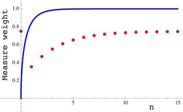
Figure 1: The two measures for the sequence $x_{n}=n+\epsilon$, $n\geq 1$, and $x_{0}=0$ are compared through the behavior of the two functions $t\mapsto\left(1-\epsilon\frac{\Gamma(\epsilon,t)}{\Gamma(1+\epsilon)}\right)$ (continuous line) and $t\mapsto\frac{\widetilde{\mathcal{N}}(t)}{\mu_{0}\,\mathcal{N}(t)}$ (dot line) for $t\geq 0$. The value of $\epsilon$ has been chosen $\epsilon=0.5$.

A second example which is interesting to study is the particular case of (6) for which $a=d=0$ and $b/c=-\epsilon$, where $\epsilon$ is a small real parameter. In that case,

$$x_{n}=n(1-\frac{\epsilon}{n^{2}})\,,\quad n\geq 1\,,\ x_{0}=0\,,$$ (77)

$$x_{n}!=\frac{\Gamma(1-\sqrt{e}+n)\,\Gamma(1+\sqrt{e}+n)}{\Gamma(1-\sqrt{e})\,\Gamma(1+\sqrt{e})\,n!}\,$$ (78)

and

$$\mathcal{N}(t)=\,\,_{2}F_{2}(1,1;1-\sqrt{e},1+\sqrt{e};t)\,,$$ (79)

where ${}_{2}F_{2}(a_{1},a_{2};b_{1},b_{2};t)$ is a generalized hypergeometric function.

As a matter of fact, the hypergeometric functions ${}_{1}F_{1}(1;b;t)$ and ${}_{2}F_{2}(1,1;b_{1},b_{2};t)$ are particular cases of a more general class of functions which also yield perturbations of the exponential function, that is, ${}_{q}F_{q}(1_{1},1_{2},...1_{q};b_{1},b_{2},...b_{q};t)$, that are connected to Delone sequences of the form $x_{n}=n+\alpha^{(q)}(n)$, with

$$\alpha^{(q)}(n)=\frac{\prod_{i=1}^{q}(n-b_{i})-n^{q}}{n^{q-1}}\,\,.$$ (80)

For these sequences,

$$x_{n}!=\frac{\prod_{i=1}^{q}\frac{\Gamma(1-b_{i}+n)}{\Gamma(1-b_{i})}}{(n!)^{q-1}}\,\,,$$ (81)

which gives for $\mathcal{N}(t)$ exactly the generalized hypergeometric function, that is,

$$\mathcal{N}(t)=\,_{q}F_{q}(\,\underset{q-times}{\underbrace{1,1,...,1}};1-b_{1},1-b_{2},...1-b_{q};t)\,\,.$$ (82)

When $q=1$ and $b_{1}=-a$, we have

$$x_{n}=n+a\,,\quad n\geq 1\,,\ x_{0}=0\,,$$ (83)

and

$$\mathcal{N}(t)=\,_{1}F_{1}(1;1+a;t)\,\,;$$ (84)

for $q=2$,

$$x_{n}=\frac{(n-b_{1})(n-b_{2})}{n}\,,\quad n\geq 1\,,\ x_{0}=0\,,$$ (85)

and

$$\mathcal{N}(t)=\,_{2}F_{2}(1,1;1-b_{1},1-b_{2};t)\,\,.$$ (86)

The example (77) solved above is a $q=2$ case, with $a_{1}=\sqrt{\epsilon}$ and $a_{2}=-\sqrt{\epsilon}$.

There are sequences still more general than (80) that result in perturbations of the exponential $\mathcal{N}(t)$, that is,

$$\alpha^{(q)}(n)=n\frac{\prod_{i=1}^{q}(n-b_{i})-\prod_{i=1}^{q}(n-a_{i})}{\prod_{i=1}^{q}(n-a_{i})}\,\,.$$ (87)

The Delone sequences for appropriate values of the constants $\{a_{i}\}$ and $\{b_{i}\}$ are then

$$x_{n}=n\frac{\prod_{i=1}^{q}(n-b_{i})}{\prod_{i=1}^{q}(n-a_{i})}\,,\quad n\geq 1\,,\ x_{0}=0\,,$$ (88)

and our “perturbed exponential” becomes

$$\mathcal{N}(t)=\,_{q}F_{q}(1-a_{1},1-a_{2},...,1-a_{q};1-b_{1},1-b_{2},...,1-b_{q};t)\,\,.$$ (89)

The Delone sequence (65) is a particular case of (88) with $q=1$, $a_{1}=1-a$ and $b_{1}=1-a-\epsilon$. The constants $\{a_{i}\}$ and $\{b_{i}\}$ have to be chosen in such a way that the values of $\alpha^{(q)}(n)$ satisfy the criteria required by the Delone sequences, for any value of $n$.

8.3 Asymptotic estimates

Let us now analyze the asymptotic behavior of some sequences presented in the last paragrah for very large values of $n$.

As a first example, let us take the Delone sequence (65) for the special value $a=1$, i.e. the constant shift for $n\geq 1$. In (74), note that the numerator is the Gamma distribution which is centered around a value of $t$ of the order of $n$. When we consider the limit for very large $n$, only large values of $t$ contribute to the integral. But, for these values of $t$,

$$\frac{\epsilon\,\Gamma(\epsilon,t)}{\Gamma(\epsilon+1)}<<1\,\,\,,$$ (90)

and we have for $\mu_{n}$ the approximate expression

$$\mu_{n}\cong 1+\frac{\epsilon\,\,\Gamma(n+2\epsilon+1)}{\Gamma(\epsilon+1)\,\Gamma(n+\epsilon+2)\,2^{n+2\epsilon}}\,F(1,1-\epsilon;n+\epsilon+2;-1)\,\,.$$ (91)

For large n, the hypergeometric function $F(1,1-\epsilon;n+\epsilon+2;-1)$ becomes a finite series; as $n$ is much larger than $\epsilon$, we can keep only its first term. Therefore, we finally obtain that the asymptotic expression for $\mu_{n}$ is

$$\mu_{n}\,\,\,\underset{n\rightarrow\infty}{\longrightarrow}\,\,1+\frac{1}{\Gamma(\epsilon)\,n\,2^{n}}\,\,,$$ (92)

which is pratically $1$ for $n=10$. In order to have a better idea of the perturbation in the spectrum $\tilde{x}_{n}$ introduced by $\mu_{n}$, (see equation (27)), we show in Figure 2 the behavior of $x_{n}-\tilde{x}_{n}$ for the first 15 values of $n$ ($\epsilon=0.1$).

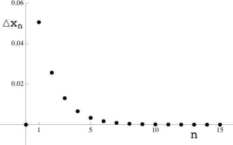
Figure 2: Delone sequence $x_{n}=n+\epsilon\,\,,n\geq 1$, and $x_{0}=0$. Behavior of $x_{n}-\tilde{x}_{n}$ for the first 15 values of $n\geq 0$ ($\epsilon=0.1$).

As a second example, let us consider the particular case of (6) for which $a=d=0$ and $b/c=-\epsilon$, where $\epsilon$ is a small real parameter. In this case, $x_{n}$ is given by the equation (77), which leads to $x_{n}!$ and $\mathcal{N}(t)$ shown by Equations (78) and (79). $\mu_{n}$ can then be written as

$$\mu_{n}=\frac{1}{x_{n}!}\int_{0}^{\infty}\frac{t^{n}dt}{{}_{2}F_{2}(1,1;1-\sqrt{\epsilon},1+\sqrt{\epsilon};t)}\,.$$ (93)

For large values of $n$, the main contribution for the integral of the previous equation is given by $t\sim n$ and the dominant contribution of the hypergeometric for $t>>1$ is

$$_{2}F_{2}(1,1;1-\sqrt{\epsilon},1+\sqrt{\epsilon};t)\underset{t>>1}{\sim}\Gamma\left[1-\sqrt{\epsilon}\right]\Gamma\left[1+\sqrt{\epsilon}\right]e^{t}\left(1-\frac{\epsilon}{t}-\frac{(1-\epsilon)\epsilon}{2t^{2}}\right)\,,$$ (94)

leading to the following asymptotic behavior for $\mu_{n}$:

$$\mu_{n}\underset{n\rightarrow\infty}{\longrightarrow}1+\frac{\epsilon}{n^{2}}\,,$$ (95)

that presents the same behavior of $x_{n}/n$ in function of $n$ as shown in Equation (77).

A more complicated example of a Delone sequence with a decay in $n$ similar to the first example of this subsection but presenting an oscillating character, is the sequence given by the following expression for $\alpha(n)$:

$$\alpha(n)=\frac{\epsilon\sin(\sqrt{2}\,n)}{n}\,,$$ (96)

where $\epsilon$ is a small parameter. In this case, $x_{n}!$, $\mathcal{N}(t)$ and $\mu_{n}$ can be calculated only numerically. We have found that the sequence $\mu_{n}$ oscillates, and the asymptotic behavior of its maxima is $|\mu_{n}-1|\equiv\epsilon/n$. In Figure 3 we show $\mu_{n}$ for the first $300$ values of $n$, taking $\epsilon=0.1$ in (96).

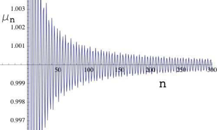
Figure 3: Delone sequence $x_{n}=n+0.1\,\dfrac{\sin{\sqrt{2}n}}{n}\,,\quad n\geq 1\,,\ x_{0}=0$. Behavior of $\mu_{n}$, for the first 300 values of $n\geq 1$. The large oscillations present near the origin have been truncated for convenience.

9 Sequences and triplets: a general algebraic setting

9.1 Heisenberg-like triplet

Suppose we are given a finite or infinite, sequence of nonnegative real numbers, bounded from below, $\{x_{n}\}_{n\in\mathbb{N}}$ such that $x_{0}=0$. Let us view this sequence as the set of eigenvalues for a positive self-adjoint operator denoted by $x_{N}$.

$$x_{N}e_{n}=x_{n}e_{n}.$$ (97)

The associated separable Hilbert space ${\cal H}$ is precisely the closure of the linear span of the orthonormal system $\{e_{n}\}$, i.e. the latter is an orthonormal basis for ${\cal H}$. We now define the operator labeling the states, or number operator, by $N$,

$$Ne_{n}=ne_{n},$$ (98)

providing also the rationale for the notation $x_{N}$, or more generally of the notation $f(N)$ for any diagonal real operator defined by $f(N)e_{n}=f(n)e_{n}$ constructed from a sequence $n\rightarrow f(n)$. The set $\mathbb{R}^{\mathbb{N}}$ of these sequences is a commutative algebra on $\mathbb{R}$, and this naturally induces a structure of a real commutative algebra for the corresponding set of $f(N)$. This algebra will be denoted by ${\cal D}$. We now define lowering and raising operators for the sequence $\{x(n)\}$:

$$a\,e_{n}=\sqrt{x_{n}}e_{n-1}\,,\quad a^{\dagger}\,e_{n}=\sqrt{x_{n+1}}e_{n+1}\,.$$ (99)

From these definitions it is clear that

$$x_{N}=a^{{\dagger}}a.$$ (100)

Now, for any diagonal operator $f(N)$ in ${\cal D}$, the following commutation rules hold:

$$af(N)=f(N+1)a\equiv f_{(-1)}(N)a,\ f(N)a^{\dagger}=a^{\dagger}f_{(-1)}(N),$$ (101)

$$[a,f(N)]=f^{\prime}(N)a=af_{(1)}^{\prime}(N),\ [a^{\dagger},f(N)]=-a^{\dagger}f^{\prime}(N)=-f_{(1)}^{\prime}(N)a^{\dagger},$$ (102)

where $f_{(m)}(N)\equiv f(N-m),\,m\in\mathbb{Z}$, is the $m^{\mbox{th}}$ shift of $f$, with the convention that $f(n)=0$ for $n<0$, and $f^{\prime}(N)\equiv f(N+1)-f(N)$ is the finite difference derivative of $f(N)$. Of course, the validity (or otherwise) of the above relations depend on domain considerations for the operators in question. In particular, we also have

$$[a,a^{\dagger}]=x^{\prime}_{N}.$$ (103)

The triplet (lowering $a$, raising $a^{{\dagger}}$, commutator $[a,a^{{\dagger}}]=x^{\prime}_{N}$) will be called a spectrum generating triplet of the sequence $\{x_{n}\}$. In [Gazeau,Lafortune,Winternitz(2008)] the Lie algebra generated by such a triplet has been investigated in a systematic way .

9.2 Generalized Heisenberg triplet

An algebraic structure which contains $q$-oscillators as a particular case was proposed in [Curado,Rego-Monteiro(2001)] and has been successfully used in some different physical problems [Oliveira-Neto et al(2007), de Souza et al(2006), Bezerra,Curado,Rego-Monteiro(2002), Ribeiro-Silva,Curado,Rego-Monteiro(2008), Curado,Rego-Monteiro(2006), Curado et al(2008)]. In this new algebra, called Generalized Heisenberg Algebra (GHA), the commutation relations among the operators $a$, $a^{\dagger}$ and a diagonal operator $J_{0}$ which is going to replace in the present context $x_{N}$ introduced in (100) depend on a general functional $h(x)$ and are given by:

$$J_{0}a^{\dagger}=a^{\dagger}h(J_{0})$$ (104)

$$aJ_{0}=h(J_{0})a$$ (105)

$$[a,a^{\dagger}]=h(J_{0})-J_{0},$$ (106)

with $a=(a^{\dagger})^{\dagger}$ and $J_{0}=J_{0}^{{\dagger}}$. This algebra tells us that the $J_{0}$ eigenvalues ($J_{0}\,e_{n}=t_{n}\,e_{n}$) are obtained by a one-step recurrence relation ($t_{n}=h(t_{n-1})$), i.e, each eigenvalue depends on the previous one. Thus, the eigenvalue behavior can be studied by dynamical system techniques, simplifying the task of finding possible representations of the algebra [Curado,Rego-Monteiro(2001)]. In order to relate this algebra to a physical system, the $J_{0}$ operator can be identified with the Hamiltonian of the system.

When the functional $h(x)$ is linear we recover [Curado,Rego-Monteiro(2001)] the $q$-oscillator algebra; other types of functionals lead to other different algebraic structures [Curado et al(2001)]. The functional $h(x)$ can be, for example, a polynomial and hence depend on some parameters (the polynomial coefficients). Let us consider the vector $e_{0}$, with the lowest eigenvalue of $J_{0}$, $J_{0}\,e_{0}=t_{0}\,e_{0}$. For a general $h(x)$, these operators act on the Fock space as

$$J_{0}\,e_{m} = h^{(m)}(t_{0})\,e_{m},\;\;\;m=0,1,2,\cdots\;,$$ (107)

$$a^{\dagger}\,e_{m} = N_{m}\,e_{m+1},$$ (108)

$$a\,e_{m} = N_{m-1}\,e_{m-1},$$ (109)

where $N_{m-1}^{2}=h^{(m)}(t_{0})-t_{0}$ and $h^{(m)}(t_{0})$ is the $m$-th iteration of $t_{0}$ by means of the function $h$.

It is interesting to observe that in some cases we can find a GHA associated to Delone perturbations of $\mathbb{N}$. Indeed, let us consider those Delone sequences, eq. (5), that can be inverted. In those cases we can write

$$n=x_{n}+\gamma(x_{n})\,.$$ (110)

Note that the difference $(x_{n}-n)$ implies that $\gamma(x_{n})$ shares the same properties as $\alpha(n)$. Therefore, the inverse sequence is also a Delone sequence.

In order to find the GHA for invertible Delone sequences, we write the $(n+1)$-st term of the sequence in terms of $x_{n}$:

$$x_{n+1}=x_{n}+1+\delta(x_{n})\,,$$ (111)

where

$$\delta(x_{n})=\gamma(x_{n})+\alpha(x_{n}+1+\gamma(x_{n}))\,.$$ (112)

The characteristic function is trivially obtained from eq. (112):

$$h(x)=x+1+\delta(x)\,,$$ (113)

and the corresponding GHA is then

$$[J_{0},A^{\dagger}]=A^{\dagger}(1+\delta(J_{0}))$$ (114)

$$[a,a^{\dagger}]=1+\delta(J_{0})\,.$$ (115)

From eqs. (5) and (110) it can be seen that $\alpha$ and $\gamma$ are perturbations of opposite signs. Thus $\delta$ is the difference of two perturbation terms and hence itself a perturbation. Eqs. (114) and (115) show that the invertible Delone sequences associated to GHA are perturbations of the quantum harmonic oscillator.

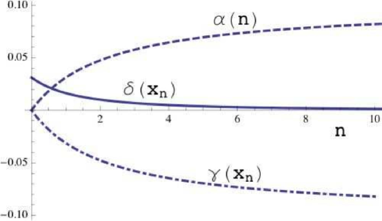
Figure 4: Delone sequence $x_{n}=n+\alpha(n)$ with $\alpha(n)=\frac{an}{cn+d}$, for the case $a=0.1$, $c=1$, and $d=2.2$. The behavior of $\alpha(n)$ (dashed line), $\delta(x_{n})$ (continuous line) and $\gamma(x_{n})$ (dot-dashed line) is shown for the first 10 values of $n$.

We take as an example of an invertible Delone sequence the case

$$\alpha(n)=\frac{an}{cn+d}\,,\quad n\geq 0\,,\quad d\neq 0\,,$$ (116)

where the real constants $a$, $c$ and $d$ have to satisfy the following conditions:

$$\left|\frac{a}{c}\right|<1;\,\,\,\,\,\,c\neq 0;\,\,\,\,\,-\frac{4}{c^{2}}\,ad\geq r-1\,,$$ (117)

and $r\in(0,1)$, according to Definition 2.1.

For this sequence,

$$\gamma(x_{n})=\frac{\sqrt{c^{2}x_{n}^{2}+2c(d-a)x_{n}+(a+d)^{2}}-cx_{n}-a-d}{2c}$$ (118)

and

$$\delta(x)=\gamma(x)+\frac{a(x+\gamma(x))+a}{c(x+\gamma(x))+c+d}\,.$$ (119)

For the particular case $x_{n}=n+\alpha(n)$ with $\alpha(n)=\frac{an}{cn+d}$, see Figure 4 where the functions $\alpha$, $\gamma$ and $\delta$ are explicitly exhibited.

If we choose specifically $a=\epsilon$, $|\epsilon|<1$, $c=1$ and $d=0$, then $\alpha(n)=\epsilon$, $\delta=0$ and the GHA is given by $h(x)=x+1$ which would characterize the harmonic oscillator algebra. However this sequence is out the scope of the present paper since $x_{0}=\epsilon\neq 0$. Imposing $x_{0}=0$ besides $x_{n}=n+\epsilon$ for $n\geq 1$ takes us to the case already examined in the previous section and for which we do not have a GHA algebraic structure.

10 A result on asymptotic Poisson and Gamma distributions

Let us now present a result which explains the behavior of the sequence $(\mu_{n})$ given a certain class of Delone sequences, namely the existence of $\mu_{\infty}$ for $\alpha$-Delone perturbations of $\mathbb{N}$. For an $\alpha$-Delone perturbation $x_{n}=n+\alpha(n)$ of $\mathbb{N}$ one can write

$$x_{n}!=n!\,\frac{1}{\xi(n)}\quad\mbox{with}\quad\frac{1}{\xi(n)}\stackrel{{\scriptstyle\mathrm{def}}}{{=}}\prod_{k=1}^{n}\left(1+\frac{\alpha(k)}{k}\right)\,.$$ (120)

Then the associated “exponential” reads as

$$\mathcal{N}(t)=\sum_{n=0}^{\infty}\frac{t^{n}}{n!}\,\xi(n)\,,$$

Its ratio to the ordinary exponential reads as the Poisson average of the random variable $n\mapsto\xi(n)$

$$\mathcal{N}(t)\,e^{-t}=\sum_{n=0}^{\infty}\frac{t^{n}}{n!}\,e^{-t}\xi(n)\stackrel{{\scriptstyle\mathrm{def}}}{{=}}(\mathrm{E}_{P}\xi)(t)\,,$$

Thus, the ratio $\mu_{n}/\xi(n)$ can be rewritten as the Gamma average of the random variable $t\mapsto e^{t}/\mathcal{N}(t)$ :

$$\frac{\mu_{n}}{\xi(n)}=\frac{1}{\xi(n)}\int_{0}^{+\infty}\frac{dt}{\mathcal{N}(t)}\,\frac{t^{n}}{x_{n}!}=\int_{0}^{\infty}\frac{t^{n}}{n!}\,e^{-t}\,\frac{e^{t}}{\mathcal{N}(t)}\,dt\stackrel{{\scriptstyle\mathrm{def}}}{{=}}\left(\mathrm{E}_{G}\frac{1}{(\mathrm{E}_{P}\xi)(t)}\right)(n)\,.$$

Let us put this on a more general setting. Let $\mathbb{N}\ni n\mapsto\xi(n)$ be a discrete function which is extendable to a function $\mathbb{R}^{+}\ni x\mapsto\mathbb{R}$ with $\xi(0)=1$ and $\lim_{x\to\infty}\xi(x)=0.$ Its Poisson mean value with parameter $t$ is given by

$$(\mathrm{E}_{P}\xi)(t):=\sum_{n=0}^{\infty}\frac{t^{n}}{n!}\,e^{-t}\xi(n)\,,$$ (121)

whereas the Gamma mean value with parameter $m$ of a random variable $\Xi$ is given by

$$(\mathrm{E}_{G}\Xi)(m)=\int_{0}^{\infty}\frac{t^{m}}{m!}\,e^{-t}\Xi(t)\,dt\,.$$ (122)

Let us examine the asymptotic behavior of the following combination of these two averages:

$$\mathrm{I}_{m}=\xi(m)\,\left(\mathrm{E}_{G}\frac{1}{(\mathrm{E}_{P}\xi)}\right)(m)=\int_{0}^{\infty}\dfrac{\dfrac{t^{m}}{m!}\,\xi(m)}{\sum_{n=0}^{\infty}\dfrac{t^{n}}{n!}\,\xi(n)}\,dt\,.$$ (123)

We would like to give sufficient conditions for having $\lim_{m\to\infty}\mathrm{I}_{m}=1$.

Proposition 10.1

Let us define the logarithm of $1/\xi$ by $\phi$ :

$$\xi(x)=e^{-\phi(x)}\,,$$ (124)

and suppose that the function $\mathbb{R}^{+}\ni x\mapsto\phi(x)$ has the following properties.

• $\phi(x)$ is three-times derivable almost everywhere (a.e.) on $\mathbb{R}^{+}$,

• $|\phi^{\prime}(x)|\ll 1$(a.e.) at large $x$. Also $x|\phi^{\prime\prime}(x)|\ll 1$(a.e.) and $x^{2}|\phi^{\prime\prime\prime}(x)|\ll 1$(a.e.) at large $x$.

Then $\mathrm{I}_{m}\underset{m\to\infty}{\to}1\,.$

Proof.  
Let us put

$$A(t)\equiv\sum_{n=0}^{\infty}\frac{t^{n}}{n!}\,\xi(n)=\frac{1}{\sqrt{2\pi}}\sum_{n=0}^{\infty}e^{F_{t}(n)},$$

with $\xi(x)\equiv e^{-\phi(x)}$ and

$$F_{t}(x):=x\ln{\frac{t}{x}}+x-\frac{1}{2}\ln{x}-\phi(x)$$ (125)

where we have neglected the errors in the Stirling’s formula, $n^{n}e^{-n}(\sqrt{2\pi n})/n!=1+{\cal O}(n^{-1})$ (e.g. ${\cal O}(n^{-1})=-0.012$ for $n=7$.) It then follows

$$F_{t}^{\prime}(x)=\ln{\frac{t}{x}}-\frac{1}{2x}-\phi^{\prime}(x)\,,\quad F_{t}^{\prime\prime}(x)=-\frac{1}{x}+\frac{1}{2x^{2}}-\phi^{\prime\prime}(x)\,.$$

We assume that there exists a solution to $F_{t}^{\prime}(x)=0$ at $x=x^{\ast}(t)$. This implies

$$x^{\ast}e^{\frac{1}{2x^{\ast}}+\phi^{\prime}(x^{\ast})}=t.$$ (126)

We now impose two conditions. Requirement 1:We demand that [$t\to\infty$] implies [$x^{\ast}(t)$ exists and that $x^{\ast}(t)\to\infty$]

In order for $x^{\ast}(t)$ to exist at large $t$, the function $xe^{\frac{1}{2x}+\phi^{\prime}(x)}$ needs to be unbounded. We face two cases:

• (Case-a) If it diverges for finite $x$ due to a singular behavior of $\phi^{\prime}(x)$, then the second condition ($x^{\ast}(t)\to\infty$) is violated. Therefore this case is excluded, i.e. $\phi^{\prime}(x)$ should be locally bounded.

• (Case-b) The asymptotic behavior of $\phi(x)$ for $x\gg 1$ is such that it allows the divergence of $xe^{\frac{1}{2x}+\phi^{\prime}(x)}$ in this limit, i.e. $\phi^{\prime}(x)$ can be negatively large but it does not dominate $\ln x$. That is, either [$\phi^{\prime}(x)>0$ ] or [$\phi^{\prime}(x)<0$ and $|\phi^{\prime}(x)|\ll\ln x$] for $x\gg 1$.

In summary

$$\phi^{\prime}(x)\geq-\ln x+\mbox{(positive increasing)}\quad(\mbox{for }x\to\infty)$$

The condition for $\phi(x)$ in the hypothesis is modest enough to satisfy the above condition.

Requirement 2: For $x^{\ast}\gg 1$, the second derivative at the peak $|F_{t}^{\prime\prime}(x^{\ast})|$ is negative, and

$$|F_{t}^{\prime\prime}(x^{\ast})|^{-\frac{1}{2}}\ll x^{\ast}$$

so that the hump of the exponential becomes asymptotically sharp. The above inequality is equivalent to (assuming that the negative value condition is satisfied)

$$\frac{1}{x}+\phi^{\prime\prime}(x)\gg\frac{1}{x^{2}}.$$

The second derivative $\phi^{\prime\prime}(x)$ can be negative, but does not dominate or cancel the $\frac{1}{x}$. We formulate this condition as

$$\phi^{\prime\prime}(x)\geq-\frac{1}{x}+\eta(x),\quad\eta(x)\gg\frac{1}{x^{2}}\quad(\mbox{for }x\to\infty)$$

The condition for $\phi(x)$ in the hypothesis is modest enough to satisfy the above condition.

Application of the Laplace method: With the above two requirements being satisfied, the evaluation of the sum is done by using

$$e^{F_{t}(x)}\simeq e^{F_{t}(x^{\ast})}e^{-\dfrac{1}{2}\,|F_{t}^{\prime\prime}(x^{\ast})|\,(x-x^{\ast})^{2}}.$$

The result is

$$A(t)\simeq\frac{\mathrm{exp}{(\frac{1}{2}+x^{\ast}\,\phi^{\prime}(x^{\ast})+x^{\ast}-\phi(x^{\ast}))}}{\sqrt{1+x^{\ast}\phi^{\prime\prime}(x^{\ast})}}\,$$

Note that $\frac{1}{\sqrt{1+x^{\ast}\phi^{\prime\prime}(x^{\ast})}}\ll\sqrt{x^{\ast}}.$

Next we evaluate

$$\mathrm{I}_{m}=\int_{0}^{\infty}\frac{t^{m}\xi(m)}{m!A(t)}dt\simeq\frac{1}{\sqrt{2\pi m}}\int_{0}^{\infty}e^{G(t)}dt,$$

with

$$G(t) = m\ln\frac{t}{m}+m-\phi(m)-\ln A(t)$$ (127)

$$\simeq m\ln\frac{t}{m}+(m-x^{\ast})-[\phi(m)-\phi(x^{\ast})]$$ (129)

$$-\frac{1}{2}-x^{\ast}\phi^{\prime}(x^{\ast})+\frac{1}{2}\ln(1+x^{\ast}\phi^{\prime\prime}(x^{\ast}))$$

The time derivative of the defining equation of $x^{\ast}$ (eq.126) gives

$$\frac{dx^{\ast}}{dt}=\frac{e^{\frac{1}{2x^{\ast}}+\phi^{\prime}(x^{\ast})}}{1+x^{\ast}\phi^{\prime\prime}(x^{\ast})}\quad(\mbox{for }t\to\infty)$$

Then

$$G^{\prime}(t) = \frac{m}{t}+\frac{dx^{\ast}}{dt}\left[-(1+x^{\ast}\phi^{\prime\prime}(x^{\ast}))+\frac{\phi^{\prime\prime}(x^{\ast})+x^{\ast}\phi^{\prime\prime\prime}(x^{\ast})}{2(1+x^{\ast}\phi^{\prime\prime}(x^{\ast}))}\right]$$ (130)

$$= \frac{m}{t}+e^{\frac{1}{2x^{\ast}}+\phi^{\prime}(x^{\ast})}\left[-1+\frac{\phi^{\prime\prime}(x^{\ast})+x^{\ast}\phi^{\prime\prime\prime}(x^{\ast})}{2(1+x^{\ast}\phi^{\prime\prime}(x^{\ast}))^{2}}\right]$$ (131)

Note that the denominator in [ ] is such that $(1+x^{\ast}\phi^{\prime\prime}(x^{\ast}))^{-2}\ll x^{\ast}$.
Final concession: Here we shall introduce further simplifying assumptions (at the possible cost of narrowing the validity region of $\phi(x)$):

$$x^{\ast}\phi^{\prime\prime}(x^{\ast})+{x^{\ast}}^{2}\phi^{\prime\prime\prime}(x^{\ast})\to 0\quad(\mbox{for }t\to\infty)$$

$$\frac{1}{2x^{\ast}}+\phi^{\prime}(x^{\ast})\to 0\quad(\mbox{for }t\to\infty)$$

These conditions are just fulfilled under the hypotheses of the proposition.
Second application of the Laplace method: Then we have first $x^{\ast}\simeq t$ asymptotically, and $G^{\prime}(t)\simeq\frac{m}{t}-1.$ Therefore,

$$G^{\prime}(m)=0\quad(\mbox{for }t\to\infty)$$

and $G^{\prime\prime}(t)=-\frac{m}{t^{2}}$ gives

$$G^{\prime\prime}(m)=-\frac{1}{m}.$$

The Laplace method then yields

$$\mathrm{I}_{m}\simeq\frac{1}{\sqrt{2\pi m}}\int_{0}^{\infty}e^{G(t)}dt\simeq\frac{1}{\sqrt{2\pi m}}\int_{-\infty}^{\infty}e^{\frac{(t-m)^{2}}{2m}}dt=1.$$

Implications : As for $\xi(m)=e^{-\phi(m)}$, the conditions

$$\phi^{\prime}(x)\to 0,\quad x\phi^{\prime\prime}(x)\to 0,\quad x^{2}\phi^{\prime\prime\prime}(x)\to 0\quad(\mbox{for }t\to\infty)$$

are rather loose. $\phi(x)=(-a)\ln x$ with both $a>0$ and $a<0$ are permissible. That is $\xi(m)$ can grow or decrease as a power law, $\xi(m)\sim x^{a}.$ So $\phi(x)=ax^{q}$ with $q<1$ and both $a>0$ and $a<0$ are admissible. That is, $\xi(m)$ can even grow like $e^{am^{q}}$ with $a>0$ and $q<1$.

11 Application to Delone $\alpha$-perturbations of $\mathbb{N}$

Let us consider an $\alpha$-perturbation of $\mathbb{N}$

$$x_{n}=n+\alpha(n)\,,\quad n\in\mathbb{N}\,,$$ (132)

where $\mathbb{N}\ni n\mapsto\alpha(n)$ is a bounded function with values in the interval $(-1,1)$, $\alpha(0)=0$, and such that its successive jumps $\alpha(n+1)-\alpha(n)$ have lower bound $r-1$ with $r\in(0,1)$.

One can write $x_{n}!=n!\,\frac{1}{\xi(n)}$ with

$$\frac{1}{\xi(n)}=\prod_{k=1}^{n}\left(1+\frac{\alpha(k)}{k}\right)\,.$$

Then the logarithm of $1/\xi$ reads as :

$$\phi(n)=\sum_{k=1}^{n}\ln{\left(1+\frac{\alpha(k)}{k}\right)}\,.$$ (133)

Let us extend the discrete domain of this function to a continuous one by replacing the sum by the integral

$$\phi(x)=\int_{1}^{x}\ln{\left(1+\frac{\alpha(y)}{y}\right)}\,dy\,.$$ (134)

Hence,

$$\phi^{\prime}(x)=\ln{\left(1+\frac{\alpha(x)}{x}\right)}\,\underset{\mbox{at large $x$}}{\approx}\frac{\alpha(x)}{x}$$ (135)

and so $\phi^{\prime}(x)\to_{x\to\infty}0$ since $x\mapsto\alpha(x)$ is bounded. For the second derivative, we have

$$\phi^{\prime\prime}(x)=\frac{x\alpha^{\prime}(x)-\alpha(x)}{x^{2}+x\alpha(x)}\,\underset{\mbox{at large $x$}}{\approx}\frac{\alpha^{\prime}(x)}{x}\,.$$ (136)

Therefore, from Proposition 10.1 one can assert the following.

Proposition 11.1

Let $x_{n}=n+\alpha(n)\,,\,n\in\mathbb{N}\,,$ an $\alpha$-perturbation of $\mathbb{N}$ such that the map $\mathbb{N}\ni n\mapsto\alpha(n)$ extends to a function $\mathbb{R}^{+}\ni x\mapsto\alpha(x)$ that is a.e. two times derivable. Suppose that $|\alpha^{\prime}(x)|\ll 1$ and $x|\alpha^{\prime\prime}(x)|\ll 1$ at large $x$. Then we have

$$\mathrm{I}_{m}=\int_{0}^{\infty}\dfrac{\dfrac{t^{m}}{x_{m}!}}{\sum_{n=0}^{\infty}\dfrac{t^{n}}{x_{n}!}}\,dt\,\to_{m\to\infty}\,1\,.$$ (137)

An example of such a sequence is given by the periodic function :

$$\mathbb{R}_{\ast}^{+}\ni x\mapsto\alpha(x)=\lambda\{\mu x\}+\nu\,,$$ (138)

with $|\lambda|<\frac{r-1}{2}\,,\,r\in(0,1)$, $|\alpha^{\prime}(x)|=|\lambda\mu|$ a.e., $\alpha^{\prime\prime}(x)=0$ a.e., and

$$\begin{array}[]{ccc}-1<\nu<1-\lambda&\mbox{if}&\lambda>0\,,\\ -\lambda-1<\nu<1&\mbox{if}&\lambda<0\,.\end{array}$$

Note that the sequences $\mathbb{Z}_{\beta}^{+}/c_{\beta}$ of rescaled non-negative $\beta$-integers with $\beta$ a quadratic PV unit, such they are defined in Proposition 2.1, are of this type and so fulfill the conditions of Proposition 11.1.

12 Discussion and outlook

In this work we have explored the possibility of quantizing the complex plane through the use of sequences of numbers close enough to the natural numbers. We have discussed the probabilistic content of the procedure. Some algebraic aspects have also been considered. We have treated a specific example, the hypergeometric case, which leads to explicit estimates. A general mathematical result has also been presented which pertains to the present context as well as to mathematical statistics. Many aspects of our work deserve further investigation, on different levels, numerical, mathematical, and interpretational, specially those around the notion of quantum or fuzzy localization in the complex plane arising from such a “non-commutative” reading of the complex plane.

Let us just discuss, from a more oriented physical point of view, the relations between the original sequence $\mathcal{X}=\{x_{n}\,,\,n\in\mathbb{N}\}$, its renormalized companion $\widetilde{\mathcal{X}}=\{\tilde{x}_{n}\,,\,n\in\mathbb{N}\}$ and the modified Lebesgue measure on the complex plane, $\nu(dz)=\dfrac{\widetilde{\mathcal{N}}(|z|^{2})}{\mathcal{N}(|z|^{2})}\,\dfrac{d^{2}z}{\mu_{0}\,\pi}$. Suppose we observe through some experimental device the sequence of numbers $\mathcal{X}$, for instance the quantum energy spectrum of a given system, that lies in the class of $\alpha$-perturbation of the nonnegative integers. Due to this proximity, probably the considered system is classically described by a harmonic oscillator with Hamiltonian $H=\frac{1}{2}(p^{2}+q^{2})$. Since the canonical quantization of the harmonic oscillator yields the integers as a spectrum, we here attempted to set up a quantization framework which takes account of the modified spectrum. For this purpose, we need to solve a Stieltjes moment problem. We know that this is impossible for most of sequences $\mathcal{X}$, for instance the sequences of rescaled beta-integers mentioned in this paper. Hence we are naturally led to deal with the renormalized sequence $\widetilde{\mathcal{X}}$ for which we solve the moment problem with the measure $\dfrac{\widetilde{\mathcal{N}}(t)}{\mathcal{N}(t)}\,\dfrac{dt}{\mu_{0}}$. This measure endows the complex plane viewed as the phase space for the harmonic oscillator with a statistical content, in the sense that classical states are not anymore described by points $z_{0}$, i. e. by Dirac distributions $z\mapsto\delta_{z_{0}}(z)$, but instead by a smooth distribution of the type $z\mapsto\dfrac{\widetilde{\mathcal{N}}(|z-z_{0}|^{2})}{\mathcal{N}(|z-z_{0}|^{2})}$. Then, by following the CS quantization stemming from the renormalized sequence, we consistently find the latter as the renormalized version of the observed spectrum along the equation

$$\widetilde{A}_{\frac{1}{2}(p^{2}+q^{2})}=\widetilde{A}_{z\bar{z}}=\tilde{a}\,\tilde{a}^{{\dagger}}=\tilde{x}_{N+1}\,.$$

This spectrum is not the observed one, but it might differ appreciably of the later in the first levels only, since $\tilde{x}_{n}=(\mu_{n}/\mu_{n-1})\,x_{n}$. Actually only the differences $\tilde{x}_{n+m}-\tilde{x}_{n}$ are experimentally significant and we should reasonably expect that they are practically the same as $x_{n+m}-x_{n}$ for excited levels, as it can be observed in the particular example shown in Figure 2.

Acknowledgements

The authors are indebted to B. Heller for fruitful comments and bibliographic suggestions. J.P.G. acknowledges the Centro Brasileiro de Pesquisas Físicas (CBPF) for financial support.

References

- [Ali et al(2000)] Ali, S. T., Antoine, J.-P., & Gazeau, J.-P., Coherent states, wavelets and their generalizations, Graduate Texts in Contemporary Physics, Springer-Verlag (New York, 2000).
- [Ali,Gazeau,Heller(2008)] Ali, S. T., Heller, B., & Gazeau, J.-P., Coherent States and Bayesian Duality, 2008, J. Phys. A: Math. Theor., 41, 365302 1-22.
- [Balkova(2008)] Balková, L., Gazeau, J.P., & Pelantová, E., Asymptotic behavior of beta-integers, 2008, Lett. Math. Phys., 84, 179-198.
- [Bardwell,Crow(1964)] Bardwell, G. E., & Crow, E. L., A Two-Parameter of Hyper-Poisson Distributions, 1964, J. Am. Stat. Association, 59, 133-141.
- [Berezin(1975)] Berezin, F. A., General concept of quantization, 1975, Comm. Math. Phys., 40, 153-174.
- [Bezerra,Curado,Rego-Monteiro(2002)] Bezerra , V. B., Curado, E. M. F., & Rego-Monteiro, M. A. , Perturbative computation in a generalized quantum field theory, Phys. Rev. D, 66, 085013 1-9.
- [Borzov(2001)] Borzov, V.V., Orthogonal polynomials and generalized oscillator algebras, Integral Transforms Spec. Funct., 12, 115-138.
- [Chakraborty et al(2008)] Chakraborty, B., Gazeau, J.P., & Youssef, A., Standard coherent state quantization of functions and distributions, submitted.
- [Curado,Rego-Monteiro(2001)] Curado, E. M. F., & Rego-Monteiro, M. A., Multi-parametric deformed Heisenberg algebra: a route to complexity, J. Phys. A: Math. Gen., 34, 3253-3264.
- [Curado et al(2001)] Curado, E. M. F., Rego-Monteiro, M. A., & Nazareno, Heisenberg-type structure of one-dimensional quantum Hamiltonian, H. N., Phys. Rev. A, 64, 012105 1-5.
- [Curado,Rego-Monteiro(2006)] Curado, E. M. F., Rego-Monteiro, M. A., Rodrigues L. M. C. S., & Hassouni, Y., Coherent states for a degenerate system: the Hydrogen atom, Physica A, 371, 16-19.
- [Curado et al(2008)] Curado, E. M. F., Hassouni, Y., Rego-Monteiro, M. A., & Rodrigues, L. M. C. S., Generalized Heisenberg algebra and algebraic methods: the example of an infinite square-well potential, Phys. Lett. A, 372, 3350-3355.
- [de Souza et al(2006)] de Souza, J., Oliveira-Neto, N. M., & Ribeiro-Silva, C. I., A method based on a nonlinear generalized Heisenberg algebra to study the molecular vibrational spectrum, Eur. Phys. J. D, 40, 205-210.
- [Erdelyi(1956)] A. Erdelyi, Asymptotic expansions, Dover, New York (1956).
- [Gazeau(2006)] Gazeau, J. P., Verger-Gaugry, J. L.: Diffraction spectra of weighted Delone sets on beta-lattices with beta a quadratic unitary Pisot number, Annales de l’Institut Fourier, 56, 2437-2461.
- [Gazeau et al(2003)] Gazeau, J-P. , Garidi, T., Huguet, E., Lachièze-Rey, M., & Renaud, J., Examples of Berezin-Toeplitz quantization: Finite sets and Unit Interval, 2003, Symmetry in Physics. In memory of Robert T. Sharp, Ed. Winternitz, P., (Montréal: CRM Proceedings and Lecture Notes 2004).
- [Gazeau,Klauder(1999)] Gazeau, J-P. , Klauder, J., Coherent States for Systems with Discrete and Continuous Spectrum, 1999 J. Phys. A: Math. Gen., 32, 123-132.
- [Gazeau,Lafortune,Winternitz(2008)] Gazeau, J-P. , Lafortune, S., & Winternitz, P., Algebras generated by spectrum generating triplets, in preparation.
- [Klauder(1963)] Klauder, J. R., Continuous-Representation Theory I. Postulates of continuous-representation theory, 1963, J. Math. Phys., 4, 1055-1058; Continuous-Representation Theory II. Generalized relation between quantum and classical dynamics, 1963, J. Math. Phys., 4, 1058-1073.
- [Klauder,Skagerstam(1985)] Klauder, J. R., & Skagerstam, B. S., Coherent States - Applications in Physics and Mathematical Physics, World Scientific, (Singapore, 1985).
- [Klauder(1995)] Klauder, J. R., Quantization without Quantization, 1995, Ann. of Phys., 237, 147-160.
- [Lieb(1994)] See Lieb, E., in Feng, D. H., Klauder, J. R., & M. Strayer (eds.) : Coherent States: Past, Present and Future, World Scientific, (Singapore, 1994).
- [Madore(1995)] Madore, J.,An Introduction to Noncommutative Differential Geometry and its Physical Applications, Cambridge University Press (Cambridge, 1995).
- [Magnus et al(1966)] Magnus, W., Oberhettinger, F., & Soni, R. P., Formulas and Theorems for the Special Functions of Mathematical Physics, 3rd ed., Springer-Verlag, (Berlin, Heidelberg and New York, 1966).
- [Oliveira-Neto et al(2007)] Oliveira-Neto, N. M., Curado, E. M. F., Nobre, F. D., & M. A. Rego-Monteiro, A simple model to describe low-temperature behaviour of some atoms and molecules: an application to the Hydrogen atom, 2007, J. Phys. B, 40, 1975-1989.
- [Ribeiro-Silva,Curado,Rego-Monteiro(2008)] Ribeiro-Silva, C. I., Curado, E. M. F. , & Rego-Monteiro, M. A., Deformed scalar quantum electrodynamics as a phenomenological model for composite scalar particles, 2008, J. Phys. A: Math. Theor., 41, 145404 1-18.