Quantum recoil effects in finite-time disentanglement of two distinguishable atoms

Abstract

Starting from the requirement of distinguishability of two atoms by their positions, it is shown that photon recoil has a strong influence on finite-time disentanglement and in some cases prevents its appearance. At near-field inter atomic distances well localized atoms — with maximally one atom being initially excited — may suffer disentanglement at a single finite time or even at a series of equidistant finite times, depending on their mean inter atomic distance and their initial electronic preparation.

I Introduction

As the interaction of a quantum system with its environment may be suppressed but never completely removed, the system’s coherence will always suffer a degrading, i.e. decoherence joos . Regarding the system as being composed of two distinguishable constituents, apart from the system’s coherence the entanglement schroedi between constituents also suffers a degrading. However, whereas coherence is gradually lost and asymptotically decays to zero at infinite time, entanglement may disappear even at finite time and in an abrupt way esd .

In recent years, there has been an increased interest in finite-time disentanglement with bipartite systems esd2 ; non-markovian ; tanas ; eberly3 ; orszag , a phenomenon that has also been experimentally observed almeida ; almeida2 . However, to best of our knowledge, no emphasis has been given to the question how to actually distinguish between the constituents. Their distinguishability is required to rightfully apply the concept of entanglement between them. Distinguishability requires the use of an additional degree of freedom that usually takes part in the system’s dynamics. Up to now, this somewhat hidden resource has been disregarded in the literature. However, its inclusion is required for a complete physical description. As is shown in this Letter, such a more complete physical description will lead to strong modifications with respect to the appearance of finite-time disentanglement.

The outline of the paper is as follows: In Sec. II the requirement of distinguishability of entangled atoms is developped, which shows the need for treating correctly the relative quantum motion of atoms and the photon recoil. The solution for the electronic probability amplitudes of the atoms is then obtained in Sec. III, assuming an initial single excitation in the atom-field system. Finally, the finite-time disentanglement conditions are discussed in Sec. IV and a summary and conclusions are given in Sec. V.

II Distinguishability of entangled atoms

Consider two identical two-level atoms that are supposed to be distinguishable by their positions. Maintaining distinguishability during a duration of the order of the natural lifetime $\tau_{0}$ of the electronic excited state requires that the quantum dispersion of the relative-position wave-packet be sufficiently weak. The wave-packet should be well localized at all times, otherwise the atoms could no longer be distinguished by their positions. More precisely, the condition for distinguishability of the atoms is, that within the time duration $\sim\tau_{0}$,

$$\Delta r\ll r,$$ (1)

where $\Delta r$ and $r$ are rms spread and mean of the distance between the atoms, respectively.

In the absence of relative motion, i.e. at a mean inter atomic distance $r_{0}$, the initial rms spread $\Delta r_{0}$ is enlarged by quantum dispersion during the excited-state lifetime $\tau_{0}$ to

$$\Delta r=\Delta r_{0}\sqrt{1+\left(\frac{l}{\Delta r_{0}}\right)^{4}}.$$ (2)

Here the dispersion length is defined as

$$l=\sqrt{\hbar\tau_{0}/m},$$ (3)

where $m$ is the atomic mass and $\tau_{0}=2\pi/\gamma_{0}$ with

$$\gamma_{0}=\frac{d^{2}\omega_{0}^{3}}{6\pi\epsilon_{0}\hbar c^{3}}$$ (4)

being the natural line width of the atom’s electronic transition with dipole moment $\mathbf{d}$ and transition frequency $\omega_{0}$.

Using Eq. (2), the condition (1) then leads to

$$\Delta r_{0}^{4}-\Delta r_{0}^{2}r_{0}^{2}+l^{4}\ll 0,$$ (5)

which has solutions only for mean interatomic distances $r_{0}\gg l$, which then establish limits for the rms spread:

$$\Delta r_{{\rm min}}\ll\Delta r_{0}\ll r_{0}.$$ (6)

The minimum rms spread is

$$\Delta r_{{\rm min}}=l^{2}/r_{0}\ll l,$$ (7)

which can be written as

$$\Delta r_{{\rm min}}\ll\lambda_{0}\sqrt{\frac{E_{{\rm r}}}{\hbar\gamma_{0}}}.$$ (8)

As the recoil energy $E_{{\rm r}}=(\hbar k_{0})^{2}/2m$ is typically smaller than $\hbar\gamma_{0}$, the minimum spread may still be much smaller than the transition wavelength $\lambda_{0}$ so that rather small spreads are allowed. However, a zero spread is not permitted, as then quantum dispersion would render the atoms indistinguishable. Thus, to be consistent with the requirement of the atoms being distinguishable during the excited-state lifetime $\tau_{0}$, a finite initial spread $\Delta r_{0}$ within the limits (6) is required.

III Interaction of two atoms with the electromagnetic field

III.1 Hamilton operator of the atom-field system

The Hamiltonian describing the free radiation field, the two atoms with their corresponding kinetic energies, and the atom-field interaction is

$$\hat{H}=\int d^{3}k\sum_{\sigma}\hbar ck\hat{n}_{\mathbf{k},\sigma}+\sum_{a=\pm}\hbar\omega_{0}\hat{S}_{a,z}+\frac{\hat{\mathbf{P}}^{2}}{4m}+\frac{\hat{\mathbf{p}}^{2}}{m}+\hat{V}.$$ (9)

Here $\hat{n}_{\mathbf{k},\sigma}=\hat{a}_{\mathbf{k},\sigma}^{\dagger}\hat{a}_{\mathbf{k},\sigma}$ is the photon-number operator with $\hat{a}_{\mathbf{k},\sigma}$ being the bosonic annihilation operator of a photon in mode $(\mathbf{k},\sigma)$, $\sigma$ denoting one of the two polarizations orthogonal to the wave vector $\mathbf{k}$. The electronic two-level systems with transition frequency $\omega_{0}$ are described by the pseudo spin operators $\hat{\mathbf{S}}_{a}$, where the index $a=\pm$ indicates the atom under consideration, and $\hat{\mathbf{P}}$ and $\hat{\mathbf{p}}$ are center-of-mass and relative momentum, respectively.

The interaction part $\hat{V}$ in Eq. (9) describes the photon absorption and emission processes associated with recoil on the corresponding atom. It can be written as

$$\hat{V}=\int d^{3}k\sum_{\sigma}\sum_{a=\pm}\hbar\kappa_{\mathbf{k},\sigma}\hat{S}_{a,+}\hat{a}_{\mathbf{k},\sigma}e^{i\mathbf{k}\cdot\hat{\mathbf{R}}-ia\mathbf{k}\cdot\hat{\mathbf{r}}/2}+{\rm H.a.},$$ (10)

where $\hat{\mathbf{R}}$ and $\hat{\mathbf{r}}$ are the center-of-mass and relative position of the atoms, respectively, and the vacuum Rabi frequency of the electromagnetic mode $(\mathbf{k},\sigma)$ is

$$\kappa_{\mathbf{k},\sigma}=\mathbf{d}\cdot\mathbf{e}_{\sigma}(\mathbf{k})E_{k}/\hbar,$$ (11)

with the polarization unit vector $\mathbf{e}_{\sigma}(\mathbf{k})$ and the rms electric-field vacuum fluctuation

$$E_{k}=\sqrt{\frac{\hbar ck}{16\pi^{3}\epsilon_{0}}}.$$ (12)

III.2 Wigner–Weisskopf solution for an initial single excitation

As we assume the electromagnetic field to be initially in its vacuum state with only one of the atoms being excited, we take the general form of the quantum state as:

$$|\Psi(t)\rangle=\int d^{3}p\int d^{3}P|\mathbf{p}\rangle_{{\rm rel}}\otimes|\mathbf{P}\rangle_{{\rm cm}}$$ (13)

$$\otimes\left[\sum_{a=\pm}\psi_{a}(\mathbf{p},\mathbf{P},t)|a\rangle+\int d^{3}k\sum_{\sigma}\psi_{\mathbf{k},\sigma}(\mathbf{p},\mathbf{P},t)|\mathbf{k},\sigma\rangle\right].$$

Here the state with atom $a=\pm$ being excited and no photon being present and the state with no atom being excited but a photon in mode $(\mathbf{k},\sigma)$ being present, are defined as

$$|\pm\rangle = |{\textstyle\mp\frac{1}{2}},{\textstyle\pm\frac{1}{2}}\rangle_{{\rm el}}\otimes|{\rm vac}\rangle_{{\rm em}},$$ (14)

$$|\mathbf{k},\sigma\rangle = |{\textstyle-\frac{1}{2}},{\textstyle-\frac{1}{2}}\rangle_{{\rm el}}\otimes|\mathbf{k},\sigma\rangle_{{\rm em}},$$ (15)

respectively, where

$$|m,m^{\prime}\rangle_{{\rm el}}=|m\rangle_{-}\otimes|m^{\prime}\rangle_{+}.$$ (16)

From the Schrödinger equation the equations of motion for the probability amplitudes in Eq. (13) are easily derived and Laplace transformed ($t\to s$). Eliminating then the photon probability amplitude $\psi_{\mathbf{k},\sigma}$, the equations for the probability amplitudes for one of the atoms being excited are obtained as:

$$\left[s+\Gamma(\mathbf{p}\pm\hbar\mathbf{k}/2,\mathbf{P}-\hbar\mathbf{k},s)+i\frac{p^{2}+P^{2}/4}{\hbar m}\right]\underline{\psi}_{\pm}(\mathbf{p},\mathbf{P},s)$$

$$+\int d^{3}k\gamma(\mathbf{k};\mathbf{p}\pm\hbar\mathbf{k}/2,\mathbf{P}-\hbar\mathbf{k},s)\underline{\psi}_{\mp}(\mathbf{p}\pm\hbar\mathbf{k},\mathbf{P},s)$$

$$=\psi_{\pm}(\mathbf{p},\mathbf{P},0),$$ (17)

where $\psi_{\pm}(\mathbf{p},\mathbf{P},0)$ is the initial probability amplitude at time $t=0$. The complex-valued spectral rate is defined as

$$\gamma(\mathbf{k};\mathbf{p},\mathbf{P},s)=\frac{\sum_{\sigma}\kappa_{\mathbf{k},\sigma}\kappa_{\mathbf{k},\sigma}^{\ast}}{s+i[ck-\omega_{0}+(p^{2}+P^{2}/4)/\hbar m]},$$ (18)

with the integrated rate being

$$\Gamma(\mathbf{p},\mathbf{P},s)=\int d^{3}k\gamma(\mathbf{k};\mathbf{p},\mathbf{P},s).$$ (19)

Given that relative and center-of-mass kinetic energies, as well as the recoil energy $E_{{\rm r}}$, typically produce frequency shifts much smaller than the natural line width $\gamma_{0}$,

$$\frac{p^{2}}{m},\frac{P^{2}}{4m},E_{{\rm r}}\ll\hbar\gamma_{0},$$ (20)

the required rates in Eq. (17) can be approximated as being independent of the atoms momenta,

$$\gamma(\mathbf{k};\mathbf{p}\pm\hbar\mathbf{k}/2,-\hbar\mathbf{k},s)\approx\gamma(\mathbf{k};s)=\frac{\sum_{\sigma}\kappa_{\mathbf{k},\sigma}\kappa_{\mathbf{k},\sigma}^{\ast}}{s+i(ck-\omega_{0})},$$ (21)

and correspondingly

$$\Gamma(\mathbf{p}\pm\hbar\mathbf{k}/2,\mathbf{P}-\hbar\mathbf{k},s)\approx\Gamma(s)=\int d^{3}k\gamma(\mathbf{k};s).$$ (22)

Using the approximated rates (21) and (22), Eqs (17) can be diagonalized by the use of the amplitudes

$$\underline{\phi}_{\pm}(\mathbf{p},\mathbf{P},s)=\frac{\underline{\psi}_{+}(\mathbf{p},\mathbf{P},s)\pm\underline{\psi}_{-}(\mathbf{p},\mathbf{P},s)}{\sqrt{2}},$$ (23)

and Fourier transformed ($\mathbf{p}\to\mathbf{r}$, $\mathbf{P}\to\mathbf{R}$) to obtain

$$\left[s+\Gamma(s)\pm\gamma(\mathbf{r};s)-i\left(\frac{\hbar\nabla_{r}^{2}}{m}+\frac{\hbar\nabla_{R}^{2}}{4m}\right)\right]\underline{\phi}_{\pm}(\mathbf{r},\mathbf{R},s)$$

$$\qquad=\phi_{\pm}(\mathbf{r},\mathbf{R},0).$$ (24)

Non-Markovian effects non-markovian may be safely neglected by taking the limit $s\to 0$ for the Fourier transform of the rate (21), which is obtained as

$$\gamma(\mathbf{r})=\lim_{s\to 0}\gamma(\mathbf{r};s)=\gamma_{0}\left[\mu(k_{0}\mathbf{r})+i\nu(k_{0}\mathbf{r})\right].$$ (25)

Here $\mu$ and $\nu$ are given by

$$\mu(\mathbf{x}) = \frac{3}{2}\left[\left(3\varsigma-2\right)\left(\frac{\cos x}{x^{2}}-\frac{\sin x}{x^{3}}\right)+\varsigma\frac{\sin x}{x}\right],$$ (26)

$$\nu(\mathbf{x}) = \frac{3}{4}\left[\left(3\varsigma-2\right)\left(\frac{\sin x}{x^{2}}+\frac{\cos x}{x^{3}}\right)-\varsigma\frac{\cos x}{x}\right],$$ (27)

where $\varsigma=\sin^{2}\theta$ with $\theta$ being the angle between $\mathbf{x}$ and the dipole transition moment $\mathbf{d}$. Whereas the imaginary part of Eq. (25) describes the dipole-dipole interaction between the atoms, the real part is responsible for a dependence of collective spontaneous emission of both atoms on their distance and the dipole orientation lehmberg ; lehmberg2 . As $\Gamma=\gamma(\mathbf{0})$ and $\mu(\mathbf{x})\to 1$ for $x\to 0$, the real part of the integrated rate becomes $\Re(\Gamma)=\gamma_{0}$.

According to Eq. (20), the kinetic energy terms in Eq. (24) are much smaller than $\gamma_{0}$, the latter appearing in the equation via $\gamma(\mathbf{r})$ and $\Gamma$. Thus we consistently neglect those terms and obtain the solution of Eq. (24), whose inverse Laplace transform then gives the probability amplitude for atom $a=\pm$ being excited in terms of the initial amplitudes:

$$\psi_{\pm}(\mathbf{r},\mathbf{R},t)=\frac{\phi_{+}(\mathbf{r},\mathbf{R},0)e^{-\gamma(\mathbf{r})t}\pm\phi_{-}(\mathbf{r},\mathbf{R},0)e^{\gamma(\mathbf{r})t}}{\sqrt{2}}e^{-\gamma_{0}t}.$$ (28)

IV Finite-time disentanglement

IV.1 Concurrence in terms of the moments of $\mu$ and $\nu$

For obtaining the entanglement between the atoms electronic subsystems we require the reduced electronic density operator,

$$\hat{\rho}_{{\rm el}}={\rm Tr}_{{\rm rel}}{\rm Tr}_{{\rm cm}}{\rm Tr}_{{\rm em}}\left[|\Psi(t)\rangle\langle\Psi(t)|\right],$$

whose density matrix is

$$\rho_{{\rm el}}(t)=\left(\begin{array}[]{cccc}0&0&0&0\\ 0&p_{-}(t)&z(t)&0\\ 0&z^{\ast}(t)&p_{+}(t)&0\\ 0&0&0&p(t)\end{array}\right)$$ (29)

in the standard basis

$$\{|{\textstyle\frac{1}{2},{\textstyle\frac{1}{2}}\rangle},|{\textstyle\frac{1}{2},{\textstyle-\frac{1}{2}}\rangle},|{\textstyle-\frac{1}{2},{\textstyle\frac{1}{2}}\rangle},|{\textstyle-\frac{1}{2},{\textstyle-\frac{1}{2}}\rangle}\}.$$

Here $p(t)=1-p_{+}(t)-p_{-}(t)$ with $p_{a}(t)$ being the probability for atom $a=\pm$ being excited and the non-diagonal element $z$ being a coherence/correlation between the atoms. Given that initially only one excitation exists in the system, the first diagonal element in (29) vanished and thus the concurrence wooters — as a measure of entanglement — is simply

$$C(t)=2\max\{0,|z(t)|\},$$

where the non-diagonal element is obtained as

$$z(t)=\int d^{3}r\int d^{3}R\psi_{-}(\mathbf{r},\mathbf{R},t)\psi_{+}^{\ast}(\mathbf{r},\mathbf{R},t).$$ (30)

For the initial quantum state we choose a state, where relative and center-of-mass motion factorize from the possibly non-factorisable electronic state:

$$\psi_{a}(\mathbf{r},\mathbf{R},0)=\Psi_{a}\sqrt{p_{{\rm rel}}(\mathbf{r})p_{{\rm cm}}(\mathbf{R})},$$

where $p_{{\rm rel}}$ and $p_{{\rm cm}}$ is the initial probability density for the relative and center-of-mass coordinate, respectively. Using this form, the matrix element (30) results as

$$z(t) = \int d^{3}rp_{{\rm rel}}(\mathbf{r})\left\{\sum_{a=\pm}\frac{a}{2}|\Phi_{a}|^{2}e^{-2\gamma_{0}t[1+a\mu(\mathbf{r})]}\right.$$ (31)

$$\left.+i\Im\left[\Phi_{+}\Phi_{-}^{\ast}e^{-2\gamma_{0}t[1-i\nu(\mathbf{r})]}\right]\right\},$$

with the initial electronic amplitudes

$$\Phi_{\pm}=(\Psi_{+}\pm\Psi_{-})/\sqrt{2}.$$

For averaging over the inter atomic distance we choose for $p_{{\rm rel}}$ a normalized isotropic Gaussian with mean distance $\mathbf{r}_{0}$ and rms spread $\Delta r_{0}$, as introduced previously. Given that the time of disentanglement is expected to be smaller than the excited-state lifetime, i.e. $\gamma_{0}t\ll 1$, the real and imaginary parts of the coherence (31) can be obtained in second-order cumulant expansion as

$$z_{r}(t) = \frac{1}{2}\left(|\Phi_{+}|^{2}e^{-2\bar{\mu}\gamma_{0}t}-|\Phi_{-}|^{2}e^{2\bar{\mu}\gamma_{0}t}\right)$$ (32)

$$\times e^{-2[\gamma_{0}t-(\Delta\mu\gamma_{0}t)^{2}]},$$

$$z_{i}(t) = |\Phi_{+}\Phi_{-}|\sin\left(2\bar{\nu}\gamma_{0}t+\varphi\right)$$ (33)

$$\times e^{-2[\gamma_{0}t+(\Delta\nu\gamma_{0}t)^{2}]},$$

where

$$\varphi=\arg(\Phi_{+}\Phi_{-}^{\ast})$$

and the mean and variance are defined as

$$\bar{\mu} = \int d^{3}rp_{{\rm rel}}(\mathbf{r})\mu(\mathbf{r}),$$

$$\Delta\mu^{2} = \int d^{3}rp_{{\rm rel}}(\mathbf{r})\mu^{2}(\mathbf{r})-\bar{\mu}^{2},$$

and correspondingly for $\bar{\nu}$ and $\Delta\nu$.

IV.2 Generic conditions for finite-time disentanglement

Finite-time disentanglement at a time $t_{d}$ requires that

$$z_{r}(t_{d})=z_{i}(t_{d})=0.$$

Let us first consider the case where $\bar{\mu}\neq 0$. Then the real part $z_{r}$ vanishes at the single time

$$\gamma_{0}t_{d}=\ln(|\Phi_{+}|/|\Phi_{-}|)/2\bar{\mu}.$$ (34)

Thus, given $\bar{\mu}\gtrless 0$ we require an initial electronic preparation with $|\Phi_{+}|\gtrless|\Phi_{-}|$ and $|\Phi_{\pm}|\neq 0$ to obtain a positive and finite time $t_{{\rm d}}$. To accomplish also a vanishing imaginary part, $z_{i}(t_{d})=0$, the phase $\varphi$ of the initial electronic preparation has to be adopted to compensate for the accumulated phase due to the dipole-dipole interaction in the sine of Eq. (33). This condition requires the phase to be

$$\varphi=n\pi-\frac{\bar{\nu}}{\bar{\mu}}\ln(|\Phi_{+}|/|\Phi_{-}|),\qquad n\in\mathbb{Z}.$$

Therefore, there can always be found an initial electronic preparation for which finite-time disentanglement occurs at exactly one time given by Eq. (34). At this time the concurrence vanishes but immediately revives, similar to Ref. orszag .

However, if $\bar{\mu}=0$, a vanishing real part $z_{r}$ can only be obtained for

$$|\Phi_{+}|=|\Phi_{-}|,$$

corresponding to the initial electronic state

$$|\Psi\rangle_{{\rm el}}=\cos({\textstyle\frac{\varphi}{2}})|{\textstyle-\frac{1}{2}},{\textstyle\frac{1}{2}}\rangle_{{\rm el}}+i\sin({\textstyle\frac{\varphi}{2}})|{\textstyle\frac{1}{2}},{\textstyle-\frac{1}{2}}\rangle_{{\rm el}}.$$ (35)

As now $z_{r}=0$ for all times, if $\bar{\nu}\neq 0$, the time of disentanglement $t_{{\rm d}}$ will be determined by the condition $z_{i}(t_{{\rm d}})=0$, which results in

$$\gamma_{0}t_{{\rm d}}=(n\pi-\varphi)/2\bar{\nu},\qquad n\in\mathbb{Z}.$$ (36)

Thus, for $\bar{\mu}=0$ and $\bar{\nu}\neq 0$, within the range of validity $\gamma_{0}t_{{\rm d}}\ll 1$, a series of equidistant finite times of disentanglement exists given an initial state of the form (35). However, the periodic revivals of the concurrence are due to the unitary and thus coherent dipole-dipole interaction between the atoms, cf. Eq. (33). Thus, different to the usual FTD, no decoherence can be attributed to them.

On the other hand, if $\bar{\mu}=0$ and also $\bar{\nu}=0$ the condition $z_{i}(t_{{\rm d}})=0$ will lead to $\varphi=n\pi$ ($n\in\mathbb{Z}$), which corresponds for the required initial state (35) to a perfect separability of the two atoms throughout their entire evolution in time. Therefore, we conclude that for $\bar{\mu}=\bar{\nu}=0$ finite-time disentanglement does not exist.

IV.3 Dependence on distance and localization of the atoms

Let us now apply these conditions considering the actual form of the functions $\mu$ and $\nu$, and their averaging with the normalized Gaussian $p_{{\rm rel}}$ with mean distance $r_{0}$ and rms spread $\Delta r_{0}$:

Far field —

In the far field, $r_{0}\gg\lambda_{0}$, both $\mu$ and $\nu$ asymptotically decay to zero, so that as a consequence their mean values vanish, $\bar{\mu},\bar{\nu}\to 0$, quite independently of the spread $\Delta r_{0}$. Therefore, finite-time disentanglement does not exist for $r_{0}\gg\lambda_{0}$, which is in agreement with our intuition: For distances larger than the correlation length of the electromagnetic vacuum the atoms interact with two statistically independent reservoirs, in which case finite-time disentanglement does not exist if maximally one atom is initially excited.

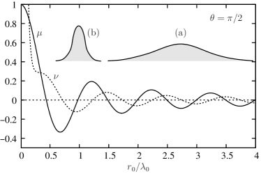
Figure 1: Dependence of $\mu$ and $\nu$ on the inter atomic distance $r$. The shaded Gaussians indicate the averaging over the inter atomic distance with $\Delta r_{0}\gg\lambda_{0}$ (a) and $\Delta r_{0}<\lambda_{0}$ (b). For angles $\theta\neq\pi/2$ a more rapid decay would be observed and at $r\to 0$ the potential energy $\propto\nu$ would be attractive instead of repulsive.

Near field —

For a mean distance of the order of the wavelength, $r_{0}\sim\lambda_{0}$, the behavior of $\mu$ and $\nu$ is dominated by oscillations with period $\lambda_{0}$, see Fig. 1. In this case, for decreasing mean distance, the atoms are supposed to start to interact with a common reservoir. There are now two possible scenarios, where $\bar{\mu}$ may vanish:

(a) The spread is $\Delta r_{0}>\lambda_{0}$ but still $\Delta r_{0}\ll r_{0}$ so that the averaging is over at least one oscillation of $\mu$ and $\nu$, leaving vanishing mean values $\bar{\mu}\approx\bar{\nu}\approx 0$, see Fig. 1 with inset (a). Also in this case finite-time disentanglement does not exist. This case corresponds to a distance between atoms, that is not well localized in space with respect to the wavelength $\lambda_{0}$, so that distance-dependent reservoir-mediated effects are washed out. This behavior has not been seen in previous work tanas ; orszag as it uniquely arises from the quantumness of atomic positions.

(b) The spread is $\Delta r_{0}<\lambda_{0}$ and $r_{0}$ is centered near to a node of $\mu$, leading to $\bar{\mu}=0$, see Fig. 1 with inset (b). As the nodes of $\nu$ are approximately shifted with respect to those of $\mu$ by $\lambda_{0}/4$, their mean will not vanish in this case: $\bar{\nu}\neq 0$. Thus, a series of equidistant finite disentanglement times according to Eq. (36) will be observed. Such a repeated disentanglement occurs also in case of two initial excitations, cf. Refs tanas ; eberly3 .

In all other cases of a near-field reservoir-mediated interaction, a single finite disentanglement time according to Eq. (34) exists. Thus, a high sensibility on the positioning and localization of the atoms in the near-field is revealed. Only for distances $r_{0}\sim\lambda_{0}$ finite-time disentanglement can exist, because only in the near field the atoms are located in a “common” reservoir. However, only well localized atoms with $\Delta r_{0}<\lambda_{0}$ can show this peculiar behavior, otherwise the distance dependent coupling is washed out. Furthermore, given well localized atoms in the near field, the number of finite disentanglement times for a given initial state depends on the precise distance between the atoms: If $r_{0}$ is at a node of $\mu$ and if the initial state is of the form (35), a series of equidistant finite disentanglement times exists. For other distances only a single finite disentanglement time exists.

V Summary and conclusions

Among the various discussions of finite-time disentanglement for two-atom systems, the work of Ficek and Tanaś tanas is closest to our approach. However, there, an initial state including two excitations, i.e. both atoms being initially excited, was studied. Moreover, the inter atomic distance was treated classically, thereby discarding quantum dispersion and photon recoil. Our results can reproduce this approximation by taking the limit $\Delta r_{0}\to 0$, which, however, is incompatible with the requirement of distinguishability, see condition (6).

A further, more drastic approximation is that of disregarding the relative position entirely and specifying either common or statistically independent reservoirs for the two atoms. Such approximations can be obtained from our results as limiting cases, further discarding the dipole-dipole interaction ($\nu\to 0$): In the limit $r_{0}\to 0$ and thus $\gamma(\mathbf{r})\to\gamma_{0}$ a common reservoir is reproduced, whereas for $r_{0}\to\infty$ and thus $\gamma(\mathbf{r})\to 0$ two statistically independent reservoirs emerge. The former case reveals finite-time disentanglement for an initial single excitation orszag . It is, however, inconsistent in discarding the dipole-dipole interaction at small distances. The latter case, on the other hand, does not show finite-time disentanglement for a single initial excitation.

In conclusion, our results offer a consistent treatment of finite-time disentanglement of two atoms with initial states containing no more than a single excitation. Only in the near field, $r_{0}\sim\lambda_{0}$, and for sufficiently well localized atoms a finite-time disentanglement can be observed. The permitted range of rms spreads is $\Delta r_{{\rm min}}\ll\Delta r_{0}<\lambda_{0}$, where the lower limit ensures the distinguishability of the atoms during the observation time and the upper limit allows for resolving the distance-dependent reservoir-mediated coupling between atoms. If the distance $r_{0}$ is at a node of $\mu$, a series of equidistant finite disentanglement times is observed for a particular type of initial electronic state, whereas for other distances only a single finite time of disentanglement can exist.

- (1) E. Joos, H.D. Zeh, C. Kiefer, D. Giulini, J. Kupsch, and I.-O. Stamatescu, Decoherence and the appearance of a classical world in quantum theory (Springer Verlag, 2003).
- (2) E. Schrödinger, Naturwissenschaften 23, 807; 823; 844 (1935).
- (3) C. Zyczowski, P. Horodecki, M. Horodecki, and R. Horodecki, Phys Rev. A. 65, 012101 (2001); L. Diósi, in Lecture Notes in Physics Vol. 622 (Springer Verlag, 2003) eds F. Benatti and R. Floreanini, p. 157; P.J. Dodd and J.J. Halliwell, Phys. Rev. A 69, 052105 (2004); T. Yu and J.H. Eberly, Phys. Rev. Lett. 93, 140404 (2004); L. Jakóbczyk and A. Jamróz, Phys. Lett. A 333, 35 (2004).
- (4) T. Yu and J.H. Eberly, Phys. Rev. Lett. 97, 140403 (2006); M. Yönaç, T. Yu and J.H. Eberly, J. Phys. B 39, S621 (2006); A. Jamróz, J. Phys. A 39, 7727 (2006); M. França Santos, P. Milman, L. Davidovich, and N. Zagury, Phys. Rev. A. 73, 040305(R), 2006; H.T. Cui, K. Li, and X.X. Yi, Phys. Lett. A 365, 44 (2007); I. Sainz and G. Björk, Phys. Rev. A 76, 042313 (2007); C.E. López, G. Romero, F. Lastra, E. Solano, and J.C. Retamal, Phys. Rev. Lett. 101, 080503 (2008).
- (5) Z. Ficek and R. Tanaś, Phys. Rev. A 74, 024304 (2006).
- (6) C. Anastopoulos, S. Shresta, and B.L. Hu, arXiv:quant-ph/0610007; X. Cao and H. Zheng, Phys. Rev. A 77, 022320 (2008).
- (7) T. Yu and J.H. Eberly, J. Mod. Opt. 54, 2289 (2007).
- (8) M. Hernández and M. Orszag, arXiv:0801.1458.
- (9) M.P. Almeida, F. de Melo, M. Hor-Meyll, A. Salles, S.P. Walborn, P.H. Souto Ribeiro, and L. Davidovich, Science 316, 579 (2007).
- (10) J. Laurat, K.S. Choi, H. Deng, C.W. Chou, and H.J. Kimble, Phys. Rev. Lett. 99, 180504 (2007).
- (11) R.H. Lehmberg, Phys. Rev. A 2, 883 (1970).
- (12) G.S. Agarwal, Quantum statistical theories of spontaneous emission and their relation to other approaches, Tracts in Modern Physics Vol. 70 (Springer Verlag, 1974).
- (13) W.K. Wooters, Phys. Rev. Lett. 80, 2245 (1998).