Photometric redshift accuracy in AKARI Deep Surveys

Abstract

We investigate the photometric redshift accuracy achievable with the AKARI infrared data in deep multi-band surveys, such as in the North Ecliptic Pole field. We demonstrate that the passage of redshifted policyclic aromatic hydrocarbons and silicate features into the mid-infrared wavelength window covered by AKARI is a valuable means to recover the redshifts of starburst galaxies. To this end we have collected a sample of $\sim$60 galaxies drawn from the GOODS-North Field with spectroscopic redshift $0.5\,\lower 2.0pt\hbox{${<\atop\hbox{\raise 4.0pt\hbox{$\sim$}}}$}\,z_{\rm spec}\,\lower 2.0pt\hbox{${<\atop\hbox{\raise 4.0pt\hbox{$\sim$}}}$}\,1.5$ and photometry from 3.6 to 24  $\mu$m, provided by the Spitzer, ISO and AKARI satellites. The infrared spectra are fitted using synthetic galaxy Spectral Energy Distributions which account for starburst and active nuclei emission. For $\sim 90\%$ of the sources in our sample the redshift is recovered with an accuracy $|z_{\rm phot}-z_{\rm spec}|/(1+z_{\rm spec})\,\lower 2.0pt\hbox{${<\atop\hbox{\raise 4.0pt\hbox{$\sim$}}}$}\,10\%$. A similar analysis performed on different sets of simulated spectra shows that the AKARI infrared data alone can provide photometric redshifts accurate to $|z_{\rm phot}-z_{\rm spec}|/(1+z_{\rm spec})\sim 10\%$ (1$\,\sigma$) at $z\,\lower 2.0pt\hbox{${<\atop\hbox{\raise 4.0pt\hbox{$\sim$}}}$}\,2$. At higher redshifts the PAH features are shifted outside the wavelength range covered by AKARI and the photo-z estimates rely on the less prominent 1.6$\,\mu$m stellar bump; the accuracy achievable in this case on $(1+z)$ is $\sim 10-15\%$, provided that the AGN contribution to the infrared emission is subdominant. Our technique is no more prone to redshift aliasing than optical-uv photo-$z$, and it may be possible to reduce this aliasing further with the addition of submillimetre and/or radio data.

1 Introduction

The discovery that infrared luminous starbursting galaxies are significant and possibly dominant contributors to the cosmic starformation history of the Universe has had an enormous impact on the understanding of galaxy evolution (Hughes et al. 1998; Lagache, Puget $\&$ Dole 2005). However, these galaxies are often too faint in the optical for large optical redshift compaigns, or have ambiguous optical identifications (Chapman et al. 2004, 2005). Attention therefore have been focusing in the last years on infrared photometric redshift estimators. Sawicki (2002) showed that the 1.6$\,\mu$m spectral feature arising from the photospheric emission from evolved stars could be used to obtain crude photometric redshift constraints with the 3.6-8.0$\,\mu$m photometry from the IRAC instrument on Spitzer. Unfortunately, the 8-24$\,\mu$m wavelength gap in Spitzer’s wide-field survey capability prevented the use of longer wavelength rest-frame features as redshift indicators, such as the much more prominent Policyclic Aromatic Hydrocarbons (PAH) and $\sim 10\,\mu$m silicate absorption features.

AKARI is a Japanese-led infrared space telescope, which was launched successfully in Feb 2006. It has undertaken deep surveys near the Ecliptic Poles, far deeper than its all-sky survey. The North Ecliptic Pole (NEP) field is the largest deep-field legacy survey of AKARI, covering $0.38$ deg², and is its major deep-field legacy (Wada et al. 2008). A wider and shallower survey at the NEP has also been performed with AKARI, over a 5.8 deg² area (Lee et al. 2008), and further deep photometric surveys have been made of well-studied Spitzer fields (Pearson et al. 2008).

AKARI observed in 9 bands from $\sim$2 up to $\sim$24$\,\mu$m. The mid-infrared imaging spans the $8-24\,\mu$m gap between Spitzer’s IRAC and MIPS instruments. The unique diagnostic power of AKARI’s Spectral Energy Distribution (SED) analysis has been confirmed by Takagi et al. (2007), who very successfully traced several starburst PAH features and identified the AGN dust torus excess over the starburst emission, obtaining at the same time a good match between the photometric redshift derived from HyperZ (Bolzonella et al. 2000) and the one obtained by fitting the infrared data with reliable starburst models.

In the present work we investigate the photometric redshift accuracy achievable with AKARI in deep multi-band surveys from infrared data alone. Infrared spectra are fitted using reference SED templates derived from the starburst model of Takagi, Arimoto $\&$ Hanami (2003, hereafter TAH03; see also Takagi, Hanami $\&$ Arimoto 2004, hereafter THA04), and already exploited in Takagi et al. (2007). However in order to deal with a possible excess over starburst emission due to an AGN activity we have included a set of reference AGN spectra derived from the model of Efstathiou $\&$ Rowan-Robinson (1995, hereafter ER95). Our photometric redshift code combines the starburst and AGN components to provide the best fit to observed or simulated spectra. We fit the infrared SEDs of a sample of galaxies with spectroscopic redshift drawn from the GOODS-North Field where deep AKARI observation have been performed at 11 and 18$\,\mu$m, and of a set of simulated spectra in the NEP Deep Field with AKARI. We aim to demonstrate in this way the power of the PAH and silicate absorption feaures to obtain reliable redshift estimates based on infrared photometry alone.

We start in Section 2 describing the reference SED templates. Section 3 presents the sample of infrared sources drawn from the GOODS-N field and Section 4 provides our results on the comparison between the photometric and the spectroscopic redshifts. Section 5 describes the simulations and the results on the photometric redshift accuracy for the AKARI NEP Deep field. Conclusions are summarized in Section 6.

2 Infrared SED templates

2.1 Starburst component

We adopt the StarBUrst with Radiative Transfer (SBURT) model of THA03 and TAH04 to deal with the infrared emission due to starburst activity.

The model deals with the star formation and chemical evolution in the starburst regions using the infall model of chemical evolution of Arimoto et al. (1992). Under the assumption that the amount of gas in the outflow from the starburst region has a negligible impact on the chemical evolution as a whole, the starburst is characterized by the rate of gas infall and that of the star-formation. However, for simplicity, THA03 set the infall time-scale equal to star-formation time-scale, $t_{0}$. The equations describing the time variation of gas mass, total stellar mass and gas metallicity are solved numerically using in input the unobscured stellar SEDs derived from the evolutionary population synthesis code of Kodama $\&$ Arimoto (1997). A top-heavy IMF is assumed with a slope $x=1.10$, flatter than the Salpeter IMF ($x=1.35$). The initial metallicity of the gas cloud, $Z_{i}$, is set to zero. According to TAH03, the chemical evolution as a function of $t/t_{0}$ as well as the properties of the SED are almost independent of the practical choice of $t_{0}$, specifically when $t_{0}\,\lower 2.0pt\hbox{${>\atop\hbox{\raise 4.0pt\hbox{$\sim$}}}$}\,50$ Myr. Therefore, all the reference SED templates used here for the starburst are calculated adopting $t_{0}=100$ Myr.

THA03 assumes a starburst region in which stars and dust are distributed within a radius $R_{\rm t}$, and introduce the following mass-radius relation

$$\frac{R_{\rm t}}{1\rm kpc}=\Theta\left(\frac{M_{\star}}{10^{9}\rm M_{\odot}}\right)^{\gamma},$$ (1)

where $\Theta$ is a compactness factor that expresss the matter concentration, with the mean density being higher for smaller values of $\Theta$, while $M_{\star}$ is the (time-dependent) total stellar mass in the starburst region. The exponent $\gamma$ is set to $\frac{1}{2}$ which results in a constant surface brightness of the straburst galaxy for constant $\Theta$. Dust is assumed to be homogeneously distributed within $R_{\rm t}$ while a King profile is adopted for the stellar density distribution. The optical depth of the starburst regions is a function of the starburst age and of the compactness factor, and increases for decreasing values of $\Theta$.

The amount of dust is given by the chemical evolution assuming a constant dust-to-metal ratio, $\delta_{0}$, with three different dust models, i.e. the model for dust in the Milky Way (MW), the Large Magellanic Cloud (LMC) and the Small Magellanic Cloud (SMC). The values of $\delta_{0}$ derived from the extinction curve and the spectra of cirrus emission are 0.40, 0.55 and 0.75 for the MW, LMC and SMC, respectively. The difference among the three extinction curves is attributed to the variation of the ratio of carbonaceous dust (graphite and PAHs) to silicate grain with the fraction of silicate dust grains increasing from MW to SMC model, i.e. as a function of metallicity; therefore the silicate absorption features are most prominent in the SEDs described by the SMC type dust model. The SED from ultraviolet to submillimetre wavelengths of starburst region is calculated for each starburst age, compactness parameter and extinction curve using a radiative transfer code that assumes isotropic multiple scattering and accounts for self-absorption of re-emitted energy from dust.

The absorption/emission properties of the dust are responsible for the infrared SED features of starforming galaxies: the PAHs emissions at 3.3, 6.2, 7.7, 8.6 and 11.3$\,\mu$m and the silicate resonances at 9.7 and 18$\,\mu$m. An example of starburst SED template drawn from the Takagi et al. model, showing the main infrared features, is presented in Fig. 1. The efficiency of these features as redshift indicators is what we are going to put to the test in the present work.

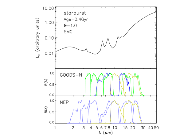
Figure 1: Example of a starburst SED template (rest-frame) drawn from the Takagi et al. model, showing the main infrared features exploited as redshift indicators: PAH emissions at 3.3, 6.2, and 7.7$\,\mu$m, and silicate absorption at 9.7$\,\mu$m. The 1.6$\,\mu$m stellar bump is also visible. In the central and in the bottom panels are shown the transmission curves of the infrared filters exploited in the GOODS-N field and in the AKARI NEP deep field, respectively, normalized to a maximum value of one: Spitzer 3.6, 4.5, 5.8, 8.0, 16 and 24$\,\mu$m filters ( green), ISO 6.5 and 15$\,\mu$m filters (blue), AKARI filters (the 11 and 18$\,\mu$m filters in yellow, the others in light blue).

2.2 AGN component

The infrared spectrum of the AGN dusty torus is modelled as in ER95. They combine an accurate solution for the axially symmetric radiative transfer problem in dust clouds with the multigrain dust model of Rowan-Robinson (1992) and three different geometries for the dusty torus that surround the central supermassive black hole. Here we assume their thick tapered disc model, which is a disc-like torus whose height increases with the distance from the central source but tapers to a constant height in the outer parts. This choice has been found to provide the best agreement with the observational constraints on AGN. The tapered disc is assumed to have a $r^{-1}$ density distribution. The ratio between the outer and the inner radius of the torus is set to 20, in the middle of the values considered by ER95, while we assume a value of 45^∘ for the half-opening angle of the torus (the values assumed by ER95 for the nucleus of NGC 1068). The equatorial optical depth of the torus is fixed to 1000. Therefore the SED of the AGN torus depends only on the viewing angle of the torus, $\theta_{view}$.
With the above choice of parameters the SED shows deep absorption features at $\sim 10\,\mu$m due to silicate dust for edge-on views of the torus ($\theta_{view}=0^{\circ}$), but it is rather featureless when the torus is seen face-on ($\theta_{view}=90^{\circ}$).

2.3 Reference SED templates and fitting procedure

Using the models described above we have created a set of reference SED templates meant for fitting any set of infrared photometric data (both real and simulated). These templates have been derived as follows (see TAH04).

• STARBURST component: for each type of extinction curve, we adopt 10 different starburst ages in the interval $t/t_{0}=0.1-6.0$ (or equivalently $t=10-600$ Myr, being $t_{0}=100$ Myr), and 17 different compactness factors in the range $\Theta=0.3-5$.

• AGN component: we vary the viewing angle between 0^∘ and 90^∘, with 11 discrete values.

The resulting SED templates are convolved with the response functions of the instruments for different values of the redshift in the range $z=0-7$ and in steps of 0.02. The fluxes derived for the two SED components (i.e. starburst and AGN torus) are then linearly combined to give the predicted flux at the passbands of the instruments. The best fit parameters of the SED models, including the redshift, are then obtained by minimizing the $\chi^{2}$

$$\chi^{2}=\sum_{i=1}^{N_{\rm filters}}\left[\frac{F_{\rm obs}(i)-\sum_{k=1}^{2}f_{k}\times F_{k}(i)}{\sigma(i)}\right]^{2},$$ (2)

where $F_{\rm obs}(i)$ is the measured flux in the passband $i$ and $\sigma(i)$ is its corresponding uncertainty. $F_{k}(i)$ represents the predicted flux in the passband $i$ contributed by the SED component $k$, with $k=1$, 2 denoting “Starburst” and “AGN”, respectively. $f_{k}$ is therefore the relative contribution of the $k$ component to the total bolometric luminosity of the galaxy. Note that for each set of values of the SED model parameters, the values of $f_{1}$ and $f_{2}$ are fixed by the condition of minimization with the restriction that they must be all non-negative. When a negative value is obtained for either $f_{1}$ or $f_{2}$, then that parameter is set to zero and the process of minimization is performed on the other SED component alone. We descard those sets of values of the SED model parameters for which the bolometric luminosity resulting from the minimization over the parameters $f_{1}$ and $f_{2}$ lies above $10^{14}$ L_⊙ or below 10⁸ L_⊙. Since we are dealing with photometric data from different telescopes we have set a minimum error of 10$\%$ on the measured fluxes before performing the SED fitting.
The goodness of the fit is described by the probability for a $\chi^{2}$-distribution, with the number of degree of freedom set by the problem, to produce a value of $\chi^{2}$ higher than the one obtained by the best SED-fit. The number of degree of freedom is given by $\nu=n_{\rm data}-n_{\rm par}$ where $n_{\rm data}$ is the number of fitted data (ranging from 8 to 10 depending on the availability of ISO and/or IRS photometry) while $n_{\rm par}$ is the number of parameters of the model, i.e. the redshift, the normalization of the SED components and the SED model parameters. As a result $n_{\rm par}=6$ if both $f_{1}$ and $f_{2}$ are positive, otherwise $n_{\rm par}=4$ ($f_{2}=0$) or $n_{\rm par}=3$ ($f_{1}=0$). A 99$\%$ confidence interval on the estimated photometric redshift is derived by the $\Delta\chi^{2}$ method (Avni 1976), being the number of “interesting parameters” equal to 1, i.e. $z_{\rm phot}$. In this case the value of $\Delta\chi^{2}$ defining the confidence interval at 99$\%$ is 6.63. A best SED-fit is considered “good” if $P_{\chi^{2}}>1\%$.

3 Data sets

In order to show the reliability of the redshift estimates based on the PAH and silicate infrared features, we have assembled a sample of galaxies with flux measurements in the wavelength range 3.6-24 $\,\mu$m and with measured spectroscopic redshifts. The sample has been selected within the northern field of the Great Observatories Origins Deep Survey (GOODS, Dickinson et al. 2001) because of its richness in multiwavelength photometric data and spectroscopic redshifts. The GOODS observations covered two fields on the sky: a northern target area (GOODS-N) coincident with (but significantly larger than) the Hubble-Deep Field North (HDF-N, Williams et al. 1996), and a similarly sized southern field (GOODS-S) coincident with the Chandra Deep Field South (Giacconi et al. 2000). The GOODS-N field has been imaged at infrared wavelengths by different instruments: at 6.75$\,\mu$m and 15$\,\mu$m by ISOCAM on board of the Infrared Space Observatory (ISO, Kessler et al. 1996), at 3.5, 4.5, 5.8, 8$\,\mu$ and 24 $\,\mu$m by Spitzer, and, more recently, at 11 and 18$\,\mu$m by AKARI (Pearson et al. 2008). Some subregions of the GOODS-N field (including part of the HDF-N) were also imaged at 16 $\mu$m by the Spitzer Infra-Red Spectrograph (IRS) blue peak-up filter (Teplitz et al. 2005). It is these sets of infrared data we have exploited here and we provide brief descriptions below.

Table 1: Some information about the Spitzer and AKARI infrared catalogues used in the present work: observing wavelength, Full With at Half Maximum (FWHM) of the instrument, number of surces detected above 3$\sigma$, corresponding minimum source flux, and surveyed area.

instrument	waveband	FWHM	$\sharp$ sources	Smin	Area
	($\mu$m)	(arcsec)		($\mu$Jy)	(arcmin2)
Spitzer/IRAC	3.6	1.6	5792	0.52	230
Spitzer/IRAC	4.5	1.7	5576	0.53	230
Spitzer/IRAC	5.8	1.9	2328	2.74	226
Spitzer/IRAC	8.0	2.0	2186	1.80	249
AKARI/IRC	11.0	4.8	242	44.04	101
AKARI/IRC	18.0	5.7	233	96.29	115
Spitzer/MIPS	24.0	6.0	1199	80.00	254

3.1 ISO

We use the catalogue of ISO sources in the HDF-N produced by Aussel et al. (1999). The source catalogue is claimed to be $95\%$ complete at 200$\,\mu$Jy in the 15$\,\mu$m band and at 65$\,\mu$Jy in the 6.5$\mu$m band. It includes 49 objects, 42 detected only at 15$\,\mu$m, 3 at only 6.5$\,\mu$m and 4 at both wavelengths. Aussel et al. also provide an additional, less secure, list of 51 sources of which 47 are detected at 15$\,\mu$m only, 4 at 6.5$\,\mu$m only, but none in both filters. All together the two catalogues include a total of 100 objects.

3.2 Spitzer

The Spitzer data for the HDF-N are part of the GOODS Spitzer Legacy Data Products and are in the public domain. The Spitzer data sets include the images of both GOODS fields at 3.6, 4.5, 5.8, 8.0$\,\mu$m from the Infra-Red Array Camera (IRAC) and at 24$\,\mu$m from the Multiband Imaging Photometer for Spitzer (MIPS), plus a list of sources for the MIPS 24$\,\mu$m imaging. The MIPS catalogue consists of 1199 sources detected at $3\sigma$, with flux densities greater than 80$\,\mu$Jy (see Table 1), a limit where the source extraction is stated to be highly complete and reliable. Source lists for the IRAC imaging have not yet been released by the GOODS consortium. Therefore we derived our own IRAC source catalogues in GOODS-N using SExtractor (Bertin $\&$ Arnouts 1996) with the default set of values for the configuration parameters. The source fluxes and the corresponding errors have been derived from the automatic aperture magnitudes. Sources were extracted down to a minimum signal-to-noise ratio of 3. The resulting catalogues consist of 5792, 5576, 2328, 2186 sources at 3.6, 4.5, 5.8 and 8.0$\,\mu$m, respectively (see Table 1).
Imaging at 16$\,\mu$m of selected areas within the GOODS-N field have been obtained as a result of a pilot study with the Spitzer IRS (Teplitz et al. 2005). The majority of the area (30 of 35 arcmin²) reaches a 3$\sigma$ sensitivity of $\sim$75$\,\mu$Jy. Teplitz et al. (2005) detected 149 objects at 16$\,\mu$m, with flux ranging from 21$\,\mu$Jy to 1.24 mJy, and with photometry in good agreement with the 15$\,\mu$m ISO survey of the same area.

3.3 AKARI

The GOODS-N region has recently been imaged at 11$\,\mu$m and 18$\,\mu$m with the AKARI Infra-Red Camera (IRC) within the FUHYU program. FUYHU is an AKARI mission program to follow-up well-studied Spitzer fields (Pearson et al. 2008) including the GOODS-N field. This survey has mapped the Lockman-Hole and ELAIS N1 fields, other well-studied fields with sufficiently high $|\beta|$ ecliptic latitudes and consequently high AKARI visibility. The source extraction and flux calibration are described in Pearson et al. (2008), and are based partly on the source extraction methodology developed for sub-millimeter surveys (Serjeant et al. 2003). The samples comprises 242 detections at 11$\mu$m and 233 at 18$\,\mu$m respectively, with a signal-to-noise ratio higher than 3 (see Table 1).

3.4 Spectroscopic redshifts

The region around the HDF-N had been the subject of intensive spectroscopic campaigns in the 90s’ by a variety of groups using the Low Resolution Imaging Spectrograph (LRIS; Oke et al. 1995) on the Keck 10 meter telescopes. A compilation of the LRIS-spectra for 671 sources is presented in Cohen et al. (2000). Subsequently, two parallel spectroscopic projects were carried out in the GOODS area using the Deep Imaging Multi-Object Spectrograph (DEIMOS) on the Keck II telescope. The Team Keck Treasury Survey (TKTS) of the GOODS-N field (Wirth et al. 2004) has focused on an $R_{AB}<24.4$ magnitude selected sample while the survey by Cowie et al. (2004) was embedded within observations targeted at high-redshift galaxies and X-ray and radio selected galaxies. More recently, Steidel and collaborators have conducted a spectroscopic survey in the GOODS-N with the blue arm of LRIS (LRIS-B) targeting several hundreds of star-forming galaxies and AGNs at redshifts $1.4\,\lower 2.0pt\hbox{${<\atop\hbox{\raise 4.0pt\hbox{$\sim$}}}$}\,z\,\lower 2.0pt\hbox{${<\atop\hbox{\raise 4.0pt\hbox{$\sim$}}}$}\,3.0$. The source candidates for spectroscopic follow-up were pre-selected using different criteria based on their optical colours (Steidel et al. 2003, 2004; Adelberger et al. 2004). The resulting spectroscopic catalogue, presented by Reddy et al. (2006) includes 342 objects and provide for each of them both optical photometry and infrared photometry at 3.6, 4.5, 5.8, 8.0 and 24$\,\mu$m from Spitzer. We use here the compilation of redshifts assembled by the Keck Team combining all the spectroscopic surveys within the GOODS-N field produced up to the 2004, and we add to it the spectroscopic sample of Reddy et al. (2006). Note that the TKTS is based primarly on observations with the DEIMOS instrument on Keck II, whose spectral range only allows the detection of emission and absorption features from objects at $z\,\lower 2.0pt\hbox{${<\atop\hbox{\raise 4.0pt\hbox{$\sim$}}}$}\,1.2$. Conversely, the selection criteria used in the spectroscopic survey of Reddy et al. is better at identifying galaxies at $z\,\lower 2.0pt\hbox{${>\atop\hbox{\raise 4.0pt\hbox{$\sim$}}}$}\,1.4$. We found indeed that only 59 out of the 342 spectroscopic sources listed in the Reddy et al. catalogue are already included in the TKTS compendium redshift catalogue.

3.5 Optical data

Optical imaging of the GOODS-N field was obtained with the Avanced Camera for Survey (ACS) on board the Hubble Space Telescope (HST) at B, V, i^′, z^′ bands. The ACS images and the source catalogues extracted by the GOODS Team are of public domain.

Optical/near-infrared ground-based images are also available for the GOODS-N field (Capak et al. 2004). An intensive multi-color imaging survey of $\sim 0.2$ deg² centered on the HDF-N have been carried out using different instruments: the Kitt Peak National Observatory (KPNO) 4 meter telescope with the MOSAIC prime focus camera, the Subaru 8.2 meter telescope with the Suprime-Cam instrument, and the QUIRC camera on the Hawaii 2.2 meter telescope. The surveyed area is referred to as the Hawaii HDF-N (Capak et al. 2004). Data were collected in $U$, $B$, $V$, $R$, $I$ and $z^{\prime}$ bands over the whole field and in $HK^{\prime}$ over a smaller region covering the Chandra Deep Field South, down to 5$\sigma$ (AB magnitudes) limits of $27.1$, $26.9$, $26.8$, $26.6$, $25.6$, $25.4$ and $22.1$, respectively. The images and the corresponding catalogues are available on the World Wide Web.

Here, optical data are used just for comparison with the infrared imaging, but they are not exploited in the SED fit.

Table 2: List of infrared sources with spectroscopic redshift drawn from the GOODS-N field, by cross-matching the source lists of Aussel et al. (1999) and of Teplitz et al. (2005) with the Spitzer and AKARI catalogues in the same field. The source positions reported here are those of the spectroscopic counterpart.

ID	Spec. position		$z_{\rm spec}$	$F_{\rm 3.6\mu m}$	$F_{\rm 4.5\mu m}$	$F_{\rm 5.8\mu m}$	$F_{\rm 8\mu m}$	$F_{\rm 24\mu m}$	$F_{\rm 6.5\mu m}$	$F_{\rm 15\mu m}$	$F_{\rm 11\mu m}$	$F_{\rm 18\mu m}$	$F_{\rm 16\mu m}$	ISO name
	$\alpha_{\rm J2000}$	$\delta_{\rm J2000}$
	(${}^{\rm h\ m\ s}$)	(${}^{\circ}\ {}^{\prime}\ {}^{\prime\prime}$)		($\mu$Jy)	($\mu$Jy)	($\mu$Jy)	($\mu$Jy)	($\mu$Jy)	($\mu$Jy)	($\mu$Jy)	($\mu$Jy)	($\mu$Jy)	($\mu$Jy)
ID1	12 36 48.30	+62 14 26.86	0.1389	86.3${}^{+2.2}_{-2.2}$	60.1${}^{+1.7}_{-1.7}$	54.8${}^{+3.2}_{-3.2}$	386.6${}^{+4.0}_{-4.0}$	460.0${}^{+6.1}_{-6.1}$	254${}^{+71}_{-73}$	307${}^{+62}_{-67}$	364${}^{+15}_{-15}$	291${}^{+32}_{-32}$	283${}^{+20}_{-20}$	HDF$\underline{~{}}$PM3$\underline{~{}}$24
ID2	12 37 23.79	+62 10 46.35	0.1133	92.9${}^{+2.9}_{-2.9}$	62.1${}^{+2.3}_{-2.3}$	54.9${}^{+4.2}_{-4.2}$	242.3${}^{+4.2}_{-4.2}$	198${}^{+6.6}_{-6.6}$	-	-	184${}^{+16}_{-16}$	129${}^{+33}_{-33}$	141${}^{+24}_{-24}$	-
ID3	12 36 12.48	+62 11 40.79	0.2759	136.9${}^{+4.1}_{-4.1}$	127.5${}^{+3.5}_{-3.5}$	99.9${}^{+6.4}_{-6.4}$	401.9${}^{+6.1}_{-6.1}$	1240${}^{+13}_{-13}$	-	-	900${}^{+15}_{-15}$	1069${}^{+32}_{-32}$	973${}^{+27}_{-27}$	-
ID4	12 36 34.47	+62 12 13.45	0.4573	316.3${}^{+5.7}_{-5.7}$	244.5${}^{+4.5}_{-4.5}$	196.0${}^{+7.9}_{-7.9}$	338.4${}^{+5.0}_{-5.0}$	1290.0${}^{+8.8}_{-8.8}$	-	448${}^{+68}_{-59}$	858${}^{+18}_{-18}$	897${}^{+32}_{-32}$	853${}^{+32}_{-32}$	HDF$\underline{~{}}$PM3$\underline{~{}}$2
ID5	12 36 22.94	+62 15 26.97	2.5920	46.4${}^{+2.2}_{-2.2}$	51.1${}^{+1.9}_{-1.9}$	72.8${}^{+4.8}_{-4.8}$	130.1${}^{+3.0}_{-3.0}$	529.0${}^{+6.2}_{-6.2}$	-	-	159${}^{+15}_{-15}$	348${}^{+32}_{-32}$	335${}^{+29}_{-29}$	-
ID6	12 37 08.32	+62 10 56.41	0.4225	61.9${}^{+1.9}_{-1.9}$	64.5${}^{+1.9}_{-1.9}$	50.0${}^{+3.2}_{-3.2}$	183.3${}^{+3.0}_{-3.0}$	648.0${}^{+7.4}_{-7.4}$	-	-	576${}^{+15}_{-15}$	494${}^{+33}_{-33}$	423${}^{+26}_{-26}$	-
ID7	12 37 19.14	+62 11 31.58	0.5560	74.1${}^{+2.1}_{-2.1}$	52.3${}^{+1.7}_{-1.7}$	48.5${}^{+3.2}_{-3.2}$	50.7${}^{+1.7}_{-1.7}$	190.0${}^{+5.9}_{-5.9}$	-	-	171${}^{+15}_{-15}$	200${}^{+32}_{-32}$	213${}^{+24}_{-24}$	-
ID8	12 36 39.71	+62 15 26.68	0.3765	46.6${}^{+1.7}_{-1.7}$	40.3${}^{+1.5}_{-1.5}$	27.9${}^{+2.4}_{-2.4}$	66.7${}^{+1.7}_{-1.7}$	161.0${}^{+5.7}_{-5.7}$	-	-	121${}^{+15}_{-15}$	136${}^{+32}_{-32}$	121${}^{+19}_{-19}$	-
ID9	12 36 51.12	+62 10 31.23	0.4099	90.7${}^{+3.3}_{-3.3}$	91.6${}^{+2.9}_{-2.9}$	74.0${}^{+5.0}_{-5.0}$	261.1${}^{+4.6}_{-4.6}$	984${}^{+9.1}_{-9.1}$	-	341${}^{+40}_{-65}$	713${}^{+15}_{-15}$	657${}^{+33}_{-33}$	745${}^{+29}_{-29}$	HDF$\underline{~{}}$PM3$\underline{~{}}$28
ID10	12 36 03.26	+62 11 11.27	0.6382	135.2${}^{+4.1}_{-4.1}$	83.6${}^{+2.8}_{-2.8}$	97.8${}^{+6.2}_{-6.2}$	92.2${}^{+3.0}_{-3.0}$	1210.0${}^{+9.5}_{-9.5}$	-	-	608${}^{+22}_{-22}$	733${}^{+144}_{-144}$	655${}^{+33}_{-33}$	-
ID11	12 36 22.50	+62 15 44.78	0.6393	71.4${}^{+2.6}_{-2.6}$	48.5${}^{+1.8}_{-1.8}$	57.1${}^{+4.1}_{-4.1}$	67.3${}^{+2.1}_{-2.1}$	721.0${}^{+6.6}_{-6.6}$	-	-	294${}^{+15}_{-15}$	346${}^{+32}_{-32}$	390${}^{+28}_{-28}$	-
ID12	12 36 50.20	+62 08 45.09	0.4335	101.3${}^{+3.3}_{-3.3}$	86.3${}^{+2.9}_{-2.9}$	79.8${}^{+5.5}_{-5.5}$	129.9${}^{+3.6}_{-3.6}$	585.0${}^{+7.8}_{-7.8}$	-	-	323${}^{+15}_{-15}$	293${}^{+33}_{-33}$	348${}^{+20}_{-20}$	-
ID13	12 36 41.56	+62 09 48.54	0.5186	204.8${}^{+4.9}_{-4.9}$	151.7${}^{+3.8}_{-3.8}$	128.6${}^{+7.3}_{-7.3}$	152.5${}^{+4.1}_{-4.1}$	433.0${}^{+6.9}_{-6.9}$	-	-	355${}^{+15}_{-15}$	322${}^{+34}_{-34}$	327${}^{+23}_{-23}$	-
ID14	12 36 55.75	+62 09 17.80	0.4191	72.9${}^{+2.8}_{-2.8}$	71.7${}^{+2.6}_{-2.6}$	67.4${}^{+4.9}_{-4.9}$	150.6${}^{+3.7}_{-3.7}$	846.0${}^{+9.9}_{-9.9}$	-	-	411${}^{+15}_{-15}$	426${}^{+32}_{-32}$	408${}^{+21}_{-21}$	-
ID15	12 36 43.98	+62 12 50.44	0.5560	58.9${}^{+2.1}_{-2.1}$	46.9${}^{+1.8}_{-1.8}$	52.6${}^{+3.7}_{-3.7}$	64.4${}^{+2.1}_{-2.1}$	424${}^{+4.6}_{-4.6}$	$<$50	282${}^{+60}_{-64}$	281${}^{+15}_{-15}$	317${}^{+34}_{-34}$	343${}^{+22}_{-22}$	HDF$\underline{~{}}$PM3$\underline{~{}}$17
ID16	12 36 48.63	+62 09 32.55	0.5174	31.6${}^{+1.9}_{-1.9}$	25.7${}^{+1.6}_{-1.6}$	20.1${}^{+2.7}_{-2.7}$	29.8${}^{+1.8}_{-1.8}$	127.0${}^{+7.3}_{-7.3}$	-	-	86${}^{+15}_{-15}$	131${}^{+32}_{-32}$	104${}^{+16}_{-16}$	-
ID17	12 36 53.89	+62 12 54.40	0.6419	58.4${}^{+1.9}_{-1.9}$	37.3${}^{+1.4}_{-1.4}$	36.5${}^{+2.7}_{-2.7}$	25.3${}^{+1.2}_{-1.2}$	200.0${}^{+6.3}_{-6.3}$	$<$36	179${}^{+60}_{-43}$	92${}^{+15}_{-15}$	181${}^{+32}_{-32}$	207${}^{+22}_{-22}$	HDF$\underline{~{}}$PM3$\underline{~{}}$33
ID18	12 36 36.80	+62 12 13.46	0.8477	126.4${}^{+3.5}_{-3.5}$	83.7${}^{+2.7}_{-2.7}$	68.9${}^{+4.8}_{-4.8}$	50.4${}^{+2.1}_{-2.1}$	379.0${}^{+5.2}_{-5.2}$	$<$113	202${}^{+58}_{-50}$	101${}^{+15}_{-15}$	261${}^{+32}_{-32}$	300${}^{+22}_{-22}$	HDF$\underline{~{}}$PM3$\underline{~{}}$8
ID19	12 36 51.79	+62 13 54.19	0.5561	46.7${}^{+1.6}_{-1.6}$	34.8${}^{+1.3}_{-1.3}$	36.2${}^{+2.6}_{-2.6}$	42.2${}^{+1.4}_{-1.4}$	203.0${}^{+6.3}_{-6.3}$	$<$39	151${}^{+74}_{-68}$	195${}^{+15}_{-15}$	176${}^{+32}_{-32}$	185${}^{+30}_{-30}$	HDF$\underline{~{}}$PM3$\underline{~{}}$30
ID20	12 36 17.44	+62 15 51.58	0.3758	22.7${}^{+1.6}_{-1.6}$	25.9${}^{+1.5}_{-1.5}$	17.5${}^{+2.7}_{-2.7}$	54.9${}^{+2.2}_{-2.2}$	145.0${}^{+9.7}_{-9.7}$	-	-	119${}^{+25}_{-25}$	116${}^{+32}_{-32}$	95${}^{+23}_{-23}$	-
ID21	12 36 46.18	+62 11 42.41	1.0164	108.2${}^{+3.4}_{-3.4}$	79.4${}^{+2.7}_{-2.7}$	49.4${}^{+4.2}_{-4.2}$	41.5${}^{+2.0}_{-2.0}$	290.0${}^{+4.9}_{-4.9}$	88${}^{+45}_{-80}$	170${}^{+59}_{-42}$	61${}^{+15}_{-15}$	212${}^{+37}_{-37}$	275${}^{+18}_{-18}$	HDF$\underline{~{}}$PM3$\underline{~{}}$19
ID22	12 36 46.89	+62 14 47.78	0.5560	44.1${}^{+1.6}_{-1.6}$	32.2${}^{+1.3}_{-1.3}$	30.2${}^{+2.4}_{-2.4}$	33.9${}^{+1.3}_{-1.3}$	277${}^{+11}_{-11}$	$<$179	144${}^{+72}_{-47}$	66${}^{+15}_{-15}$	266${}^{+32}_{-32}$	193${}^{+17}_{-17}$	HDF$\underline{~{}}$PM3$\underline{~{}}$23
ID23	12 36 31.65	+62 16 04.41	0.7840	44.9${}^{+1.7}_{-1.7}$	30.0${}^{+1.3}_{-1.3}$	30.9${}^{+2.6}_{-2.6}$	23.8${}^{+1.2}_{-1.2}$	301${}^{+5.3}_{-5.3}$	-	-	87${}^{+15}_{-15}$	239${}^{+32}_{-32}$	245${}^{+22}_{-22}$	-
ID24	12 37 01.49	+62 08 42.37	0.7038	37.7${}^{+2.3}_{-2.3}$	20.7${}^{+1.6}_{-1.6}$	23.1${}^{+3.5}_{-3.5}$	21.3${}^{+1.9}_{-1.9}$	185.0${}^{+7.2}_{-7.2}$	-	-	70${}^{+15}_{-15}$	123${}^{+33}_{-33}$	130${}^{+24}_{-24}$	-
ID25	12 36 49.72	+62 13 13.39	0.4745	53.5${}^{+1.8}_{-1.8}$	49.0${}^{+1.6}_{-1.6}$	47.4${}^{+3.1}_{-3.1}$	113.0${}^{+2.4}_{-2.4}$	371${}^{+10}_{-10}$	136${}^{+68}_{-57}$	320${}^{+39}_{-62}$	356${}^{+15}_{-15}$	410${}^{+33}_{-33}$	370${}^{+27}_{-27}$	HDF$\underline{~{}}$PM3$\underline{~{}}$27
ID26	12 36 39.93	+62 12 50.38	0.8462	64.1${}^{+2.5}_{-2.5}$	38.9${}^{+1.7}_{-1.7}$	40.0${}^{+3.5}_{-3.5}$	30.9${}^{+1.6}_{-1.6}$	493.0${}^{+6.1}_{-6.1}$	$<$64	302${}^{+67}_{-55}$	120${}^{+15}_{-15}$	288${}^{+32}_{-32}$	425${}^{+20}_{-20}$	HDF$\underline{~{}}$PM3$\underline{~{}}$11
ID27	12 36 17.33	+62 15 29.95	0.8497	79.4${}^{+3.1}_{-3.1}$	55.8${}^{+2.2}_{-2.2}$	52.9${}^{+4.6}_{-4.6}$	31.6${}^{+1.7}_{-1.7}$	499.0${}^{+7.2}_{-7.2}$	-	-	93${}^{+15}_{-15}$	354${}^{+32}_{-32}$	448${}^{+27}_{-27}$	-
ID28	12 36 33.59	+62 13 20.24	0.8446	49.9${}^{+2.3}_{-2.3}$	32.9${}^{+1.7}_{-1.7}$	34.6${}^{+3.6}_{-3.6}$	23.1${}^{+1.5}_{-1.5}$	323.0${}^{+6.8}_{-6.8}$	-	122${}^{+54}_{-40}$	68${}^{+15}_{-15}$	192${}^{+35}_{-35}$	320${}^{+29}_{-29}$	HDF$\underline{~{}}$PS3$\underline{~{}}$3
ID29	12 36 49.50	+62 14 07.13	0.7517	32.6${}^{+1.3}_{-1.3}$	21.4${}^{+1.0}_{-1.0}$	21.7${}^{+2.0}_{-2.0}$	17.6${}^{+1.0}_{-1.0}$	186.0${}^{+6.4}_{-6.4}$	$<$40	150${}^{+74}_{-48}$	69${}^{+15}_{-15}$	143${}^{+33}_{-33}$	130${}^{+20}_{-20}$	HDF$\underline{~{}}$PM3$\underline{~{}}$26
ID30	12 36 33.66	+62 10 06.20	1.0156	72.1${}^{+3.2}_{-3.2}$	56.2${}^{+2.4}_{-2.4}$	44.0${}^{+4.1}_{-4.1}$	45.4${}^{+2.2}_{-2.2}$	581.0${}^{+9.0}_{-9.0}$	-	-	94${}^{+15}_{-15}$	398${}^{+32}_{-32}$	438${}^{+25}_{-25}$	-
ID31	12 36 33.14	+62 15 14.01	0.5196	16.7${}^{+1.1}_{-1.1}$	13.9${}^{+0.9}_{-0.9}$	13.5${}^{+1.9}_{-1.9}$	17.8${}^{+1.1}_{-1.1}$	142.0${}^{+7.0}_{-7.0}$	-	-	112${}^{+15}_{-15}$	182${}^{+32}_{-32}$	41${}^{+17}_{-17}$	-
ID32	12 36 54.81	+62 08 47.67	0.7913	64.1${}^{+2.7}_{-2.7}$	44.1${}^{+2.1}_{-2.1}$	41.9${}^{+4.0}_{-4.0}$	42.9${}^{+2.1}_{-2.1}$	246.0${}^{+5.6}_{-5.6}$	-	-	75${}^{+15}_{-15}$	102${}^{+33}_{-33}$	134${}^{+17}_{-17}$	-
ID33	12 36 46.23	+62 15 27.64	0.8510	84.5${}^{2.2}_{-2.2}$	56.7${}^{+1.7}_{-1.7}$	54.2${}^{+3.3}_{-3.3}$	42.3${}^{+1.5}_{-1.5}$	544.0${}^{+7.6}_{-7.6}$	-	418${}^{+91}_{-94}$	119${}^{+15}_{-15}$	350${}^{+32}_{-32}$	433${}^{+27}_{-27}$	HDF$\underline{~{}}$PM3$\underline{~{}}$21
ID34	12 36 55.94	+62 08 08.58	0.7920	108.5${}^{+3.9}_{-3.9}$	76.0${}^{+3.2}_{-3.2}$	73.2${}^{+6.1}_{-6.1}$	73.9${}^{+3.3}_{-3.3}$	832.0${}^{+7.5}_{-7.5}$	-	-	213${}^{+15}_{-15}$	384${}^{+32}_{-32}$	568${}^{+20}_{-20}$	-
ID35	12 36 32.48	+62 15 13.57	0.6827	34.4${}^{+1.6}_{-1.6}$	23.0${}^{+1.2}_{-1.2}$	22.8${}^{+2.3}_{-2.3}$	18.8${}^{+1.1}_{-1.1}$	142.0${}^{+6.7}_{-6.7}$	-	-	112${}^{+15}_{-15}$	182${}^{+32}_{-32}$	143${}^{+17}_{-17}$	-
ID36	12 36 31.50	+62 11 14.52	1.0124	42.8${}^{+2.1}_{-2.1}$	32.3${}^{+1.7}_{-1.7}$	27.9${}^{+3.2}_{-3.2}$	39.7${}^{+2.1}_{-2.1}$	480.0${}^{+5.9}_{-5.9}$	-	355${}^{+40}_{-60}$	75${}^{+15}_{-15}$	287${}^{+34}_{-34}$	430${}^{+20}_{-20}$	HDF$\underline{~{}}$PM3$\underline{~{}}$1
ID37	12 36 37.80	+62 11 49.70	0.8380	37.3${}^{+2.0}_{-2.0}$	31.6${}^{+1.6}_{-1.6}$	29.2${}^{+3.2}_{-3.2}$	24.6${}^{+1.8}_{-1.8}$	173.0${}^{+3.6}_{-3.6}$	$<$61	212${}^{+58}_{-55}$	81.4${}^{+15}_{-15}$	238${}^{+33}_{-33}$	142${}^{+20}_{-20}$	HDF$\underline{~{}}$PM3$\underline{~{}}$10
ID38	12 36 38.30	+62 11 51.16	0.8410	36.9${}^{+1.9}_{-1.9}$	23.3${}^{+1.4}_{-1.4}$	29.3${}^{+3.2}_{-3.2}$	16.9${}^{+1.5}_{-1.5}$	230.0${}^{+3.3}_{-3.3}$	$<$61	212${}^{+58}_{-55}$	81.4${}^{+15}_{-15}$	238${}^{+33}_{-33}$	189${}^{+19}_{-19}$	HDF$\underline{~{}}$PM3$\underline{~{}}$10
ID39	12 36 34.53	+62 12 41.34	1.2190	66.1${}^{+2.6}_{-2.6}$	71.9${}^{+2.4}_{-2.4}$	58.1${}^{+4.4}_{-4.4}$	72.6${}^{+2.4}_{-2.4}$	446.0${}^{+5.1}_{-5.1}$	-	363${}^{+79}_{-39}$	104${}^{+15}_{-15}$	705${}^{+32}_{-32}$	923${}^{+32}_{-32}$	HDF$\underline{~{}}$PM3$\underline{~{}}$3
ID40	12 36 34.86	+62 16 28.62	0.8470	58.9${}^{+1.9}_{-1.9}$	40.1${}^{+1.5}_{-1.5}$	38.5${}^{+2.8}_{-2.8}$	34.8${}^{+1.3}_{-1.3}$	482.0${}^{+4.6}_{-4.6}$	-	-	104${}^{+15}_{-15}$	300${}^{+32}_{-32}$	368${}^{+21}_{-21}$	-
ID41	12 36 35.59	+62 14 24.32	2.0050	71.6${}^{+2.4}_{-2.4}$	99.9${}^{+2.5}_{-2.5}$	163.4${}^{+6.3}_{-6.3}$	282.6${}^{+4.0}_{-4.0}$	1480${}^{+10}_{-10}$	-	441${}^{+43}_{-82}$	369${}^{+15}_{-15}$	756${}^{+32}_{-32}$	615${}^{+32}_{-32}$	HDF$\underline{~{}}$PM3$\underline{~{}}$5
ID42	12 36 41.43	+62 11 42.81	0.5480	59.9${}^{+2.5}_{-2.5}$	61.2${}^{+2.3}_{-2.3}$	46.7${}^{+4.0}_{-4.0}$	39.7${}^{+2.0}_{-2.0}$	225.0${}^{+5.0}_{-5.0}$	127${}^{+99}_{-61}$	$<$72	55${}^{+15}_{-15}$	137${}^{+33}_{-33}$	134${}^{+15}_{-15}$	HDF$\underline{~{}}$PM2$\underline{~{}}$1
ID43	12 35 56.10	+62 12 19.57	0.9585	80.4${}^{+3.1}_{-3.1}$	60.5${}^{+2.4}_{-2.4}$	53.8${}^{+4.7}_{-4.7}$	79.4${}^{+2.9}_{-2.9}$	430.0${}^{+6.1}_{-6.1}$	-	-	119${}^{+15}_{-15}$	249${}^{+34}_{-34}$	295${}^{+25}_{-25}$	-
ID44	12 36 44.35	+62 14 53.34	1.4865	13.8${}^{+0.9}_{-0.9}$	14.1${}^{+0.9}_{-0.9}$	16.8${}^{+1.9}_{-1.9}$	21.7${}^{+1.1}_{-1.1}$	81.7${}^{+6.4}_{-6.4}$	$<$329	105${}^{+94}_{-21}$	47${}^{+15}_{-15}$	133${}^{+32}_{-32}$	37${}^{+16}_{-16}$	HDF$\underline{~{}}$PM3$\underline{~{}}$18
continued on next page

Table 2: Continued

ID	Spec. position		$z_{\rm spec}$	$F_{\rm 3.6\mu m}$	$F_{\rm 4.5\mu m}$	$F_{\rm 5.8\mu m}$	$F_{\rm 8\mu m}$	$F_{\rm 24\mu m}$	$F_{\rm 6.5\mu m}$	$F_{\rm 15\mu m}$	$F_{\rm 11\mu m}$	$F_{\rm 18\mu m}$	$F_{\rm 16\mu m}$	ISO name
	$\alpha_{\rm J2000}$	$\delta_{\rm J2000}$
	(${}^{\rm h\ m\ s}$)	(${}^{\circ}\ {}^{\prime}\ {}^{\prime\prime}$)		($\mu$Jy)	($\mu$Jy)	($\mu$Jy)	($\mu$Jy)	($\mu$Jy)	($\mu$Jy)	($\mu$Jy)	($\mu$Jy)	($\mu$Jy)	($\mu$Jy)
ID45	12 36 29.16	+62 10 46.46	1.0130	98.1${}^{+3.5}_{-3.5}$	88.3${}^{+3.1}_{-3.1}$	76.0${}^{+5.3}_{-5.3}$	70.6${}^{+2.7}_{-2.7}$	724.0${}^{+12}_{-12}$	-	-	75${}^{+15}_{-15}$	434${}^{+33}_{-33}$	465${}^{+25}_{-25}$	-
ID46	12 36 46.60	+62 10 49.36	0.9399	32.6${}^{+1.9}_{-1.9}$	24.3${}^{+1.5}_{-1.5}$	24.3${}^{+3.0}_{-3.0}$	18.2${}^{+1.4}_{-1.4}$	354${}^{+6.5}_{-6.5}$	-	327${}^{+39}_{-63}$	71${}^{+15}_{-15}$	259${}^{+32}_{-32}$	315${}^{+29}_{-29}$	HDF$\underline{~{}}$PM3$\underline{~{}}$22
ID47	12 36 36.86	+62 11 35.17	0.07860	170.6${}^{+4.1}_{-4.1}$	114.9${}^{+3.1}_{-3.1}$	113.5${}^{+6.0}_{-6.0}$	545.2${}^{+6.6}_{-6.6}$	732.0${}^{+9.1}_{-9.1}$	$<$135	300${}^{+62}_{-67}$	370${}^{+15}_{-15}$	377${}^{+32}_{-32}$	-	HDF$\underline{~{}}$PM3$\underline{~{}}$7
ID48	12 36 36.64	+62 13 47.12	0.9590	78.4${}^{+2.6}_{-2.6}$	77.3${}^{+2.3}_{-2.3}$	91.1${}^{+5.0}_{-5.0}$	110.6${}^{+2.7}_{-2.7}$	474.0${}^{+5.9}_{-5.9}$	-	353${}^{+40}_{-66}$	188${}^{+15}_{-15}$	346${}^{+33}_{-33}$	-	HDF$\underline{~{}}$PM3$\underline{~{}}$6
ID49	12 37 05.87	+62 11 54.03	0.9032	83.5${}^{+2.3}_{-2.3}$	55.8${}^{+1.7}_{-1.7}$	50.4${}^{+3.1}_{-3.1}$	39.7${}^{+1.4}_{-1.4}$	655.0${}^{+8.1}_{-8.1}$	-	431${}^{+43}_{-80}$	100${}^{+15}_{-15}$	397${}^{+33}_{-33}$	-	HDF$\underline{~{}}$PM3$\underline{~{}}$45
ID50	12 36 59.92	+62 14 50.28	0.7610	50.5${}^{+1.7}_{-1.7}$	33.6${}^{+1.3}_{-1.3}$	39.3${}^{+2.7}_{-2.7}$	33.0${}^{+1.2}_{-1.2}$	466.0${}^{+5.5}_{-5.5}$	-	295${}^{+61}_{-66}$	166${}^{+15}_{-15}$	310${}^{+34}_{-34}$	-	HDF$\underline{~{}}$PM3$\underline{~{}}$40
ID51	12 36 53.21	+62 11 17.12	0.9350	83.4${}^{+2.8}_{-2.8}$	58.4${}^{+2.2}_{-2.2}$	51.5${}^{+4.1}_{-4.1}$	47.1${}^{+2.2}_{-2.2}$	367.0${}^{+6.4}_{-6.4}$	-	174${}^{+59}_{-43}$	65${}^{+15}_{-15}$	214${}^{+33}_{-33}$	-	HDF$\underline{~{}}$PM3$\underline{~{}}$31
ID52	12 36 53.37	+62 11 39.97	1.2698	32.8${}^{+1.6}_{-1.6}$	34.6${}^{+1.6}_{-1.6}$	26.4${}^{+2.7}_{-2.7}$	40.3${}^{+1.7}_{-1.7}$	322.0${}^{+6.2}_{-6.2}$	-	180${}^{+60}_{-43}$	57${}^{+15}_{-15}$	393${}^{+33}_{-33}$	-	HDF$\underline{~{}}$PM3$\underline{~{}}$32
ID53	12 36 58.99	+62 12 09.20	0.8517	62.7${}^{+2.0}_{-2.0}$	42.6${}^{+1.6}_{-1.6}$	35.1${}^{+2.7}_{-2.7}$	24.9${}^{+1.2}_{-1.2}$	269.0${}^{+6.0}_{-6.0}$	$<$66	157${}^{+75}_{-49}$	85${}^{+15}_{-15}$	179${}^{+33}_{-33}$	-	HDF$\underline{~{}}$PM3$\underline{~{}}$39
ID54	12 37 02.74	+62 14 02.02	1.2463	62.6${}^{+1.9}_{-1.9}$	60.0${}^{+1.7}_{-1.7}$	40.3${}^{+2.8}_{-2.8}$	49.5${}^{+1.6}_{-1.6}$	334.0${}^{+7.6}_{-7.6}$	-	144${}^{+73}_{-47}$	61${}^{+15}_{-15}$	417${}^{+33}_{-33}$	-	HDF$\underline{~{}}$PM3$\underline{~{}}$44
ID55	12 36 57.79	+62 14 55.28	0.8493	45.9${}^{+1.6}_{-1.6}$	31.8${}^{+1.2}_{-1.2}$	33.4${}^{+2.5}_{-2.5}$	31.0${}^{+1.2}_{-1.2}$	366.0${}^{+7.8}_{-7.8}$	-	225${}^{+60}_{-56}$	79${}^{+15}_{-15}$	258${}^{+32}_{-32}$	-	HDF$\underline{~{}}$PM3$\underline{~{}}$37
ID56	12 36 38.13	+62 11 16.44	1.0174	52.2${}^{+2.3}_{-2.3}$	39.6${}^{+1.9}_{-1.9}$	32.7${}^{+3.4}_{-3.4}$	31.9${}^{+1.9}_{-1.9}$	291.0${}^{+4.9}_{-4.9}$	-	212${}^{+58}_{-55}$	56${}^{+15}_{-15}$	287${}^{+39}_{-39}$	-	HDF$\underline{~{}}$PM3$\underline{~{}}$9
ID57	12 36 54.64	+62 11 27.43	0.2542	50.1${}^{+2.0}_{-2.0}$	43.7${}^{+1.8}_{-1.8}$	27.1${}^{+2.8}_{-2.8}$	118.2${}^{+2.9}_{-2.9}$	173.0${}^{+6.0}_{-6.0}$	-	42${}^{+29}_{-09}$	180${}^{+15}_{-15}$	103${}^{+33}_{-33}$	-	HDF$\underline{~{}}$PS3$\underline{~{}}$23
ID58	12 36 42.19	+62 15 45.77	0.8572	126.6${}^{+2.7}_{-2.7}$	102.6${}^{+2.3}_{-2.3}$	106.1${}^{+4.5}_{-4.5}$	121.0${}^{+2.3}_{-2.3}$	850.0${}^{+7.5}_{-7.5}$	-	459${}^{+46}_{-86}$	190${}^{+15}_{-15}$	457${}^{+32}_{-32}$	-	HDF$\underline{~{}}$PS3$\underline{~{}}$10
ID59	12 37 04.33	+62 14 46.58	2.2110	5.6${}^{+0.6}_{-0.6}$	8.5${}^{+0.7}_{-0.7}$	15.7${}^{+1.8}_{-1.8}$	39.5${}^{+1.4}_{-1.4}$	376.0${}^{+4.1}_{-4.1}$	-	80${}^{+74}_{-19}$	97${}^{+15}_{-15}$	187${}^{+32}_{-32}$	-	HDF$\underline{~{}}$PS3$\underline{~{}}$36

Figure 2: 20${}^{\prime\prime}\times 20^{\prime\prime}$ postage stamp images centered on the infrared sources listed in Table 2. From left to right: R and HK^′ optical images, IRAC images at 3.6, 4.5, 5.8 8.0$\,\mu$m, AKARI images at 11 and 18$\,\mu$m, and MIPS image at 24$\,\mu$m. Red dots in the Spitzer and AKARI images represent 3$\sigma$ detections at the corresponding wavebands while the circle is the “error”-circle of 2$\sigma_{\rm FWHM}$-radius used for cross-matching the spectroscopic catalogue with the infrared catalogues, i.e. 2$\sigma_{\rm FWHM}$ = 4.08^′′, 4.84^′′ and 5.10^′′ at 11, 18 and 24$\,\mu$m, respectively. A circle of $1.5^{\prime\prime}$ in the $R$ band image indicates the spectroscopic counterpart.

Figure 2: Continued.

Figure 2: Continued.

Figure 2: Continued.

3.6 Cross-matching

We have cross-matched the spectroscopic catalogues with each of the infrared catalogues mentioned above by using for the matching radius a value equal to twice the Gaussian rms width $\sigma_{\rm FWHM}$ (=FWHM/2$\sqrt{2\ln{2}}$) of the instrument beam, where $\sigma_{\rm FWHM}$ is 6.4^′′ for ISOCAM at 15$\mu$m, 0.68^′′, 0.72^′′, 0.81^′′, 0.85^′′ for IRAC at 3.6, 4.5, 5.8, 8.0$\mu$m respectively, 2.55^′′ for MIPS at 24$\mu$m, 1.53^′′ for IRS at 16 $\mu$m, 2.04^′′ and 2.42^′′ for the AKARI at 11 and 18$\mu$m, respectively. In order to ensure full spectral coverage from mid- to far-IR wavelengths we kept only spectroscopic sources with a counterpart in all of the Spitzer and AKARI infrared catalogues considered here plus a counterpart in either the ISO 15$\,\mu$m or the IRS 16$\,\mu$m catalogues. The advantage of covering the whole mid- to far-IR spectral range is made clear by looking at the middle panel of Fig. 1, where the Spitzer, AKARI and ISO filters are shown: all the main PAH and silicate features are sampled up to $z\sim 2$ with the photometric data exploited here. At $z\,\lower 2.0pt\hbox{${>\atop\hbox{\raise 4.0pt\hbox{$\sim$}}}$}\,2$ the PAH features are shifted outside the wavelength range covered by Spitzer and AKARI so that they can no longer be exploited as redshift indicators. In this case, the rest-frame 1.6$\,\mu$m bump can be used instead for photometric redshift estimates (Sawicki 2002).

We ended up with a sample of 59 objects; 22 of them have flux measurements at both 15$\,\mu$m and 16$\,\mu$m. ISO 6.5$\,\mu$m flux measurements (or upper limits) have been included, when available, in the SED fitting process. The redshifts of the sources and their infrared fluxes are listed in Table 2. We also provide in Fig. 2 postage stamp images for all the sources in our sample at $R$, $HK^{\prime}$, Spitzer and AKARI wavebands.

For almost all of the sources in the sample we found a single counterpart at each infrared waveband. However few of them appear to lie in crowded regions, possibly affecting the infrared flux at the longest wavebands, see e.g. ID3, ID20, ID25, ID31, ID35, ID37, ID38 and ID44. There are in particular pairs of objects “sharing” the same AKARI (and ISO) fluxes, i.e. ID31-ID35 and ID37-ID38. In this cases the AKARI (and ISO) photometry should be taken as an upper limit to the intrinsic flux of the source at those wavelengths.

Most of the sources in the sample lie at $z\,\lower 2.0pt\hbox{${<\atop\hbox{\raise 4.0pt\hbox{$\sim$}}}$}\,1.5$. Only 3 out of 59 have $z_{\rm spec}>1.5$: ID5 ($z_{\rm spec}=2.5920$), ID41 ($z_{\rm spec}=2.0050$) and ID59 ($z_{\rm spec}=2.2110$). We found that just five objects in the Reddy et al. catalogue have a counterpart at both 11 and 18$\,\mu$m and either at 15 or 16$\,\mu$m. They are (according to the names they have in the Reddy et al. source list): BX1321 (at z=0.139), BM1156 (at 2.211), BM1299 (at z=1.595), BM1326 (at 1.268), and MD39 (at 2.583). Four of them are in common with the TKTS spectroscopic catalogue and fall into the final sample of 59 infrared sources presented here, corresponding to ID1, ID5, ID52 and ID59. MD39 is instead missing from our final sample because it lacks a counterpart in our IRAC catalogues at both 3.6 and 8.0$\,\mu$m. MD39 appears to be the source very close to ID24 in the corresponding postage stamp image of Fig. 2, at wavelength $\lambda\,\lower 2.0pt\hbox{${<\atop\hbox{\raise 4.0pt\hbox{$\sim$}}}$}\,5.8\,\mu$m. The pair of objects is not resolved at longer wavelengths and indeed Reddy et al. do not provide a 24$\,\mu$m flux estimate for it, probably because it cannot easily be deblended from the nearby ID24 source (although they provide for it flux estimates at all the four IRAC wavebands). For this reason we have decided not to include MD39 in our final catalogue and to add instead ID24 to the list of our infrared sources with uncertain far-IR photometry.

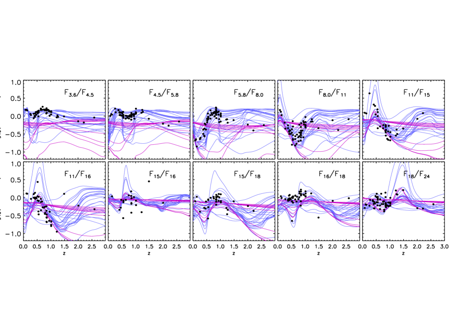
Figure 3: Observed flux ratios as a function of spectroscopic redshift (black dots) for the sample of infrared sources extracted from the GOODS-N field. Blue lines show the predicted colors from the starburst models of Takagi et al. for a subsample of representative values of the sed model parameters (see text). The predicted colors from the AGN templates exploited in the SED fitting are shown in magenta.

Fig. 3 shows the observed flux ratios as a function of the spectroscopic redshifts (black dots), and compare them to the predictions from the starburst reference templates for a representative set of SED model parameters (blue curves), and from the AGN reference templates (megenta curves). The effects of the PAH 6.2$\,\mu$m emission feature and of the 9.7$\,\mu$m silicate absorption are clearly manifest in the data. The deep “well” observed in the F_5.8/F_8.0, F_8.0/F₁₁, F₁₁/F₁₅ and F₁₁/F₁₆ diagrams at $z\sim 0.2$, $z\sim 0.6$, $z\sim 1.2$ and $z\sim 1.4$ is due to the passage of the PAH 6.2$\,\mu$m feature through the 8.0, 11, 15 and 16$\,\mu$m wavebands, respectively. The 9.7$\,\mu$m silicate absorption manifests itself as a bump in the 8.0/11$\,\mu$m flux ratios around $z\sim 0$ where the feature falls into the AKARI 11$\,\mu$m passband. As the same feature enters the 15 and 16$\,\mu$m wavebands, which occurs at $z\sim 0.5$, it produces a significant corresponding peak in the F${}_{11}/$F₁₅ and F${}_{11}/$F₁₆ diagrams. A hint of a bump due to the silicate absorption is seen also in the 15/18$\,\mu$m and 16/18$\,\mu$m flux ratios at $z\sim 0.7$, although it is not particularly prominent due to the wider wavelength coverage of the AKARI 18$\,\mu$m filter compared to the 11$\,\mu$m band. Finally, by entering the MIPS 24$\,\mu$m band, the silicate absorption induces another significant bump in the 18/24$\,\mu$m flux ratio at $z\sim 1.5$. Note that such a bump can be used for efficiently selecting ultraluminous infrared galaxies in the redshift range $1\,\lower 2.0pt\hbox{${<\atop\hbox{\raise 4.0pt\hbox{$\sim$}}}$}\,z\,\lower 2.0pt\hbox{${<\atop\hbox{\raise 4.0pt\hbox{$\sim$}}}$}\,2$ with AKARI (see Takagi $\&$ Pearson 2005). The $\sim 10\,\mu$m silicate absorption is also responsible for the behaviour in the predicted flux ratios of the AGN templates when the torus is seen edge-on. For a face-on AGN the corresponding flux ratios are almost independent of redshift, implying that for a power-law infrared spectrum the recovery of the redshift from mid-/far-IR photometry alone is extremely challenging, if not impossible.

On average the range of flux ratios spanned by the data is accounted for by the model with the sole exception of the 15/16$\,\mu$m flux ratios. Indeed we observe for few objects a significant steep increase of the flux from 15 to 16$\,\mu$m (ID28, ID39, ID42, which lie well below the theoretical expectations) or, conversely, a notable decrease of the flux when moving from 15 to 16$\,\mu$m (ID44).

4 Results of SED fitting

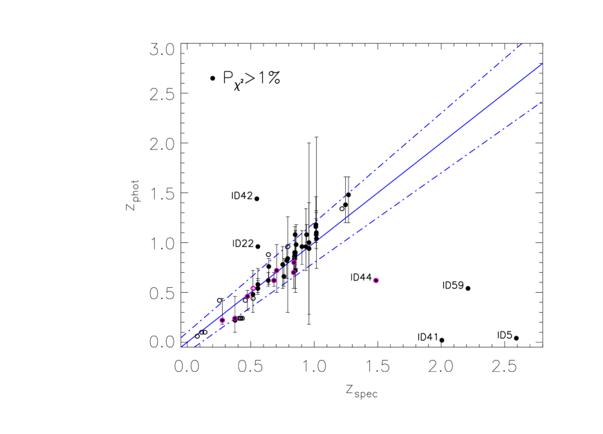
Figure 5: Photometric versus spectroscopic redshift for the sources listed in Table 2. Filled circles mark the cases of a “good” fit to the SED (i.e. $P_{\chi^{2}}>1\%$) while the open circles correspond to a bad SED fit (i.e. $P_{\chi^{2}}<1\%$). Sources with uncertain photometry at AKARI and ISO wavebands are circled in color. The dot-dashed lines delimit the region where $(z_{\rm phot}-z_{\rm spec})/(1+z_{\rm spec})<10\%$ while the solid line corresponds to the case $z_{\rm phot}=z_{\rm spec}$. Errors on photometric redshifts are in 99$\%$ confidence limit and, for reason of clarity, they are shown only for the objects with $P_{\chi^{2}}>1\%$, lying within the $10\%$-accuracy region.

The results of the SED fitting are listed in Table 3. A comparison between the photometric data and the best-fit SED model is shown in Fig. 4. The derived photometric redshifts versus the spectroscopic redshifts are presented in Fig. 5 where sources with $P_{\chi^{2}}>1\%$ are indicated by filled circles (42 in total, i.e. $\sim 70\%$ of the whole sample), and those with $P_{\chi^{2}}<1\%$ are identified by open circles. In the same figure the solid line marks the ideal case in which $z_{\rm phot}=z_{\rm spec}$, while the dot-dashed lines delimit the region where $|z_{\rm phot}-z_{\rm spec}|/(1+z_{\rm spec})<10\%$. Error bars corresponding to a 99$\%$ confidence limit have been drawn, for reason of clarity, only for objects with $P_{\chi^{2}}>1\%$ which lie within the 10$\%$ confidence region.

For almost all of the sources with $z_{\rm spec}\,\lower 2.0pt\hbox{${<\atop\hbox{\raise 4.0pt\hbox{$\sim$}}}$}\,1.5$ and $P_{\chi^{2}}>1\%$ the redshift is recovered with an accuracy $|z_{\rm phot}-z_{\rm spec}|/(1+z_{\rm spec})\,\lower 2.0pt\hbox{${<\atop\hbox{\raise 4.0pt\hbox{$\sim$}}}$}\,10\%$. The only exceptions are ID22 (at $z_{\rm spec}=0.5560$), ID42 (at $z_{\rm spec}=0.5480$) and ID44 (at $z_{\rm spec}=1.4865$).

For ID22, we would expect the PAH 6.2 and 7.7$\,\mu$m features to enter the 11$\,\mu$m AKARI filter at $z_{\rm spec}\sim 0.5$ and therefore to produce a bump in the measured flux at that waveband. This is for example what we observe in the spectrum of ID7 and ID15 whose redshifts are very close to that of ID22: a bump at 11$\mu$m followed by a plateau at longer wavelengths as a result of the convolution of the instruments filters whith the redshifted silicate absorption features at 9.7 and 18$\,\mu$m and with the PAH 11.3$\,\mu$m mission feature. On the contrary, the SED of ID22 increases monotonically in the interval 8-18$\,\mu$m. Interestingly, we found that at $z\sim 0.5$ the highest contribution to the value of the $\chi^{2}$ in Eq. 2 (after minimization over the other SED model parameters) comes from the AKARI 11$\,\mu$m waveband. By removing the data point at 11$\,\mu$m from the measured spectrum and performing the fit on the other photometric data alone we get $z_{\rm phot}=0.56$, in excellent agreement with the spectroscopic value. We also tested that none of the flux measurements at wavelengths $>11\,\mu$m have such an effect on the photo-$z$ estimate. Therefore the failure in the recovery of the redshift for ID22 seems to be determined exclusively by the AKARI photometry at 11$\,\mu$m. This result points to the conclusion that the source has an intrinsically low PAH 7.7$\,\mu$m emission that our reference SED templates are not able to account for that.

Figure 4: Comparison between the best-fit SED model (black solid curve) and the measured infrared spectrum (dots with error bars) for the infrared sources listed in Table 2. The inferred contributions from a starburst and an AGN torus, are represented by the dashed and the dot-dashed curves, respectively. Also shown are the spectroscopic redshift of the sources ($z_{\rm spec}$), the derived photometric redshifts ($z_{\rm phot}$), the corresponding value of the minimum reduced $\chi^{2}$ ($\chi^{2}_{\rm min}/\nu$) and the associated probability ($P_{\chi^{2}}$). The red solid curve is the best-fit SED model obtained by assuming a priori that the AGN component is null.

Figure 4: Continued.

Figure 4: Continued.

Figure 4: Continued.

Table 3: Best SED-fit parameters obtained for the sample of infrared sources listed in Table 2: photometric redshif ($z_{\rm phot}$, second column) with errors corresponding to a 99$\%$ confidence limit, minimum reduced $\chi^{2}$ ($\chi_{\rm min}^{2}/\nu$, third column), number of degrees of freedom ($\nu$, fourth column), probability associated to the minimum $\chi^{2}$ ($P_{\chi^{2}}$, fifth column), age of the starburst (Age, sixth column), compactness factor ($\Theta$, seventh column), extinction curve (Ext., eighth column), viewing angle of the AGN dust torus ($\theta_{\rm view}$, ninth column), luminosity contributed by the starburst component ($\log L_{\rm SB}$, tenth column), luminosity contributed by the AGN component ($\log L_{\rm AGN}$, eleventh column). The best-fit luminosities have been derived integrating the rest-frame SED from 0.1 to 1000 $\mu$m. The spectroscopic redshifts of the sources ($z_{\rm spec}$) are listed for comparison. The other columns show the results obtained by setting a priori the AGN fraction, $f_{2}$, to zero and fitting the observed SED with the starburst SED templates alone. An asterisk marks the sources with uncertain counterpart at AKARI and ISO wavebands.

ID	$z_{\rm spec}$	$z_{\rm phot}$	$\chi_{\rm min}^{2}/\nu$	$\nu$	$P_{\chi^{2}}$	Age	$\Theta$	Ext.	$\theta_{\rm view}$	$\log L_{\rm SB}$	$\log L_{\rm AGN}$	$z_{\rm phot}$	$\chi_{\rm min}^{2}/\nu$	$\nu$	$P_{\chi^{2}}$
						(Gyr)			(∘)	($L_{\odot}$)	($L_{\odot}$)
ID1	0.1389	0.10${}^{+0.04}_{-0.02}$	6.67	4	$\ll 0.01$	0.5	5.0	MW	0	10.17	6.60	0.10${}^{+0.04}_{-0.02}$	4.45	6	$\ll 0.01$
ID2	0.1133	0.10${}^{+0.04}_{-0.04}$	6.19	4	$\ll 0.01$	0.6	5.0	MW	-	10.11	-	0.10${}^{+0.04}_{-0.04}$	6.19	4	$\ll 0.01$
ID3∗	0.2759	0.22${}^{+0.22}_{-0.04}$	3.53	2	0.029	0.4	5.0	MW	27	11.09	9.52	0.24${}^{+0.14}_{-0.04}$	2.05	4	0.085
ID4	0.4573	0.42${}^{+0.08}_{-0.20}$	8.37	3	$\ll 0.01$	0.6	5.0	MW	0	11.87	10.59	0.44${}^{+0.04}_{-0.12}$	6.61	5	$\ll 0.01$
ID5	2.5920	0.04${}^{+4.96}_{-0.02}$	2.68	2	0.069	0.6	5.0	SMC	36	8.93	8.02	0.98${}^{+0.06}_{-0.06}$	7.19	4	$\ll 0.01$
ID6	0.4225	0.24${}^{+0.24}_{-0.06}$	13.31	2	$\ll 0.01$	0.6	1.8	MW	45	10.66	9.05	0.24${}^{+0.22}_{-0.04}$	7.37	4	$\ll 0.01$
ID7	0.5560	0.54${}^{+0.08}_{-0.06}$	1.71	2	0.181	0.6	3.0	MW	45	11.36	9.39	0.52${}^{+0.06}_{-0.04}$	0.97	4	0.423
ID8	0.3765	0.22${}^{+0.22}_{-0.10}$	2.41	2	0.090	0.6	5.0	MW	36	10.50	8.71	0.22${}^{+0.18}_{-0.08}$	2.14	4	0.073
ID9	0.4099	0.24${}^{+0.22}_{-0.06}$	12.87	3	$\ll 0.01$	0.4	2.6	LMC	90	10.98	9.38	0.24${}^{+0.22}_{-0.04}$	8.85	5	$\ll 0.01$
ID10	0.6382	0.62${}^{+0.08}_{-0.06}$	3.51	2	0.030	0.4	3.0	MW	0	11.81	10.86	0.60${}^{+0.12}_{-0.06}$	2.45	4	0.044
ID11	0.6393	0.88${}^{+0.08}_{-0.36}$	10.80	2	$\ll 0.01$	0.3	0.5	SMC	0	12.45	11.25	0.82${}^{+0.12}_{-0.04}$	6.05	4	$\ll 0.01$
ID12	0.4335	0.24${}^{+0.38}_{-0.10}$	11.21	2	$\ll 0.01$	0.6	2.4	LMC	45	10.87	9.38	0.90${}^{+0.06}_{-0.06}$	5.75	4	$\ll 0.01$
ID13	0.5186	0.44${}^{+0.36}_{-0.28}$	7.07	2	$\ll 0.01$	0.5	5.0	LMC	63	11.70	10.18	0.26${}^{+0.22}_{-0.06}$	4.66	4	$\ll 0.01$
ID14	0.4191	0.24${}^{+0.28}_{-0.06}$	9.79	2	$\ll 0.01$	0.4	2.6	LMC	45	10.80	9.42	0.24${}^{+0.08}_{-0.04}$	6.87	4	$\ll 0.01$
ID15	0.5560	0.58${}^{+0.16}_{-0.08}$	3.23	4	0.012	0.5	2.2	MW	81	11.36	10.09	0.54${}^{+0.06}_{-0.06}$	2.83	6	$\ll 0.01$
ID16	0.5174	0.48${}^{+0.24}_{-0.18}$	0.27	2	0.764	0.6	3.0	MW	0	10.94	9.43	0.46${}^{+0.08}_{-0.16}$	0.32	4	0.866
ID17	0.6419	0.76${}^{+0.08}_{-0.18}$	1.29	4	0.273	0.5	3.0	MW	90	11.53	8.71	0.76${}^{+0.08}_{-0.18}$	0.86	6	0.052
ID18	0.8477	0.88${}^{+0.28}_{-0.18}$	1.45	4	0.215	0.6	3.0	MW	90	11.90	9.84	0.88${}^{+0.22}_{-0.14}$	1.06	6	0.390
ID19	0.5561	0.54${}^{+0.10}_{-0.04}$	2.71	4	0.028	0.5	3.0	MW	63	11.22	9.52	0.54${}^{+0.04}_{-0.04}$	2.05	6	0.055
ID20∗	0.3758	0.24${}^{+0.22}_{-0.14}$	3.65	2	0.026	0.5	5.0	MW	36	10.32	8.87	0.28${}^{+0.16}_{-0.08}$	2.73	4	0.028
ID21	1.0164	1.10${}^{+0.22}_{-0.08}$	1.05	4	0.400	0.6	5.0	LMC	0	11.98	11.64	1.20${}^{+0.14}_{-0.28}$	1.56	6	0.154
ID22	0.5560	0.96${}^{+0.80}_{-0.30}$	0.85	4	0.494	0.3	5.0	MW	90	11.67	10.53	1.04${}^{+0.54}_{-0.30}$	1.97	6	0.067
ID23	0.7840	0.82${}^{+0.12}_{-0.18}$	1.51	2	0.221	0.4	2.6	MW	36	11.53	9.61	0.82${}^{+0.10}_{-0.12}$	0.82	4	0.512
ID24∗	0.7038	0.72${}^{+0.26}_{-0.22}$	2.10	2	0.122	0.3	2.8	LMC	36	11.39	9.92	0.58${}^{+0.26}_{-0.10}$	1.69	4	0.150
ID25∗	0.4745	0.46${}^{+0.06}_{-0.14}$	1.83	4	0.120	0.4	3.0	MW	72	11.18	9.93	0.46${}^{+0.04}_{-0.16}$	2.31	6	0.031
ID26	0.8462	0.84${}^{+0.20}_{-0.10}$	4.28	4	$<0.01$	0.4	2.8	MW	0	11.68	10.62	0.86${}^{+0.10}_{-0.12}$	3.01	6	$<0.01$
ID27	0.8497	1.08${}^{+0.10}_{-0.10}$	4.28	2	0.014	0.6	5.0	SMC	0	11.87	11.87	0.90${}^{+0.06}_{-0.12}$	3.64	4	$<0.01$
ID28	0.8446	0.86${}^{+0.36}_{-0.12}$	6.43	3	$\ll 0.01$	0.4	2.8	MW	45	11.61	7.37	0.86${}^{+0.10}_{-0.10}$	3.86	5	$<0.01$
ID29	0.7517	0.78${}^{+0.18}_{-0.24}$	0.26	4	0.902	0.5	2.2	MW	36	11.30	9.62	0.64${}^{+0.28}_{-0.10}$	0.291	6	0.941
ID30	1.0156	1.08${}^{+0.24}_{-0.14}$	1.70	2	0.182	0.3	0.9	SMC	0	12.22	11.66	1.14${}^{+0.14}_{-0.20}$	1.29	4	0.272
ID31∗	0.5196	0.54${}^{+0.14}_{-0.06}$	9.85	2	$\ll 0.01$	0.3	5.0	MW	0	10.93	9.82	0.54${}^{+0.08}_{-0.06}$	5.69	4	$\ll 0.01$
ID32	0.7913	0.84${}^{+0.42}_{-0.54}$	2.68	2	0.069	0.6	0.7	SMC	72	11.67	10.42	0.92${}^{+0.14}_{-0.10}$	2.69	4	0.029
ID33	0.8510	0.90${}^{+0.22}_{-0.12}$	3.58	3	0.013	0.4	3.0	MW	90	11.86	9.90	0.90${}^{+0.10}_{-0.10}$	2.28	5	0.044
ID34	0.7920	0.96${}^{+0.08}_{-0.18}$	9.21	2	$\ll 0.01$	0.2	0.7	SMC	0	12.61	9.62	0.96${}^{+0.06}_{-0.10}$	4.61	4	$\ll 0.01$
ID35∗	0.6827	0.62${}^{+0.08}_{-0.06}$	0.56	4	0.694	0.3	5.0	MW	-	11.29	-	0.62${}^{+0.08}_{-0.06}$	0.56	4	0.694
ID36	1.0124	1.16${}^{+0.08}_{-0.14}$	3.01	5	0.010	0.1	0.9	SMC	-	12.53	-	1.16${}^{+0.08}_{-0.08}$	3.01	5	0.010
ID37∗	0.8380	0.70${}^{+0.14}_{-0.16}$	1.52	4	0.192	0.6	1.8	MW	45	11.28	9.69	0.64${}^{+0.14}_{-0.10}$	1.34	6	0.234
ID38∗	0.8410	0.80${}^{+0.06}_{-0.10}$	0.75	6	0.609	0.4	2.4	MW	-	11.44	-	0.80${}^{+0.06}_{-0.10}$	0.75	6	0.609
ID39	1.2190	1.34${}^{+0.14}_{-0.12}$	4.26	3	$<0.01$	0.2	0.9	SMC	0	12.67	12.17	1.38${}^{+0.08}_{-0.06}$	2.86	5	0.014
ID40	0.8470	0.90${}^{+0.22}_{-0.16}$	4.65	2	$<0.01$	0.4	2.6	MW	36	11.70	10.25	0.92${}^{+0.14}_{-0.14}$	2.88	4	0.021
ID41	2.0050	0.02${}^{+0.52}_{-0.02}$	1.66	3	0.174	0.07	5.0	LMC	45	8.31	7.75	0.02${}^{+0.02}_{-0.02}$	7.57	5	$\ll 0.01$
ID42	0.5480	1.44${}^{+0.56}_{-0.64}$	1.64	4	0.162	0.2	5.0	SMC	36	12.30	11.17	1.10${}^{+0.66}_{-0.24}$	1.72	6	0.112
ID43	0.9585	1.00${}^{+0.40}_{-0.82}$	4.19	2	0.015	0.4	3.0	LMC	90	11.87	11.05	0.30${}^{+0.16}_{-0.10}$	3.86	4	$<0.01$
ID44∗	1.4865	0.62${}^{+4.38}_{-0.58}$	1.77	4	0.131	0.6	1.4	LMC	45	10.60	10.02	0.96${}^{+0.06}_{-0.24}$	2.79	6	0.010
ID45	1.0130	1.18${}^{+0.28}_{-0.14}$	3.23	2	0.040	0.2	1.2	SMC	18	12.55	11.22	1.20${}^{+0.16}_{-0.14}$	1.66	4	0.156
ID46	0.9399	1.08${}^{+0.10}_{-0.08}$	3.02	3	0.029	0.5	0.7	SMC	0	11.73	11.68	0.88${}^{+0.10}_{-0.08}$	3.28	5	$<0.01$
ID47	0.0786	0.06${}^{+0.04}_{-0.02}$	11.71	3	$\ll 0.01$	0.6	5.0	MW	0	9.96	7.33	0.06${}^{+0.04}_{-0.02}$	7.16	5	$\ll 0.01$
ID48	0.9590	0.94${}^{+1.06}_{-0.66}$	0.56	2	0.570	0.6	0.4	SMC	72	12.16	11.10	0.94${}^{+0.20}_{-0.06}$	4.69	4	$\ll 0.01$
ID49	0.9032	0.96${}^{+0.16}_{-0.18}$	2.50	2	0.082	0.5	3.0	MW	0	11.85	11.32	0.96${}^{+0.12}_{-0.10}$	1.49	4	0.202
ID50	0.7610	0.66${}^{+0.18}_{-0.10}$	1.08	2	0.339	0.3	5.0	MW	0	11.52	11.58	0.64${}^{+0.18}_{-0.08}$	0.94	4	0.442
ID51	0.9350	0.96${}^{+0.38}_{-0.24}$	1.03	2	0.356	0.3	1.8	SMC	45	12.00	10.41	1.04${}^{+0.20}_{-0.28}$	1.10	4	0.355
ID52	1.2698	1.48${}^{+0.18}_{-0.28}$	0.92	2	0.399	0.1	5.0	MW	72	12.25	11.09	1.42${}^{+0.20}_{-0.22}$	1.85	4	0.115
ID53	0.8517	0.72${}^{+0.26}_{-0.22}$	0.07	3	0.976	0.5	5.0	MW	0	11.53	10.54	0.66${}^{+0.32}_{-0.12}$	0.17	5	0.973
continued on next page

Table 3: Continued

ID	$z_{\rm spec}$	$z_{\rm phot}$	$\chi_{\rm min}^{2}/\nu$	$\nu$	$P_{\chi^{2}}$	Age	$\Theta$	Ext.	$\theta_{\rm view}$	$\log L_{\rm SB}$	$\log L_{\rm AGN}$	$z_{\rm phot}$	$\chi_{\rm min}^{2}/\nu$	$\nu$	$P_{\chi^{2}}$
						(Gyr)			(∘)	($L_{\odot}$)	($L_{\odot}$)
ID54	1.2463	1.38${}^{+0.28}_{-0.18}$	1.79	2	0.167	0.2	5.0	MW	90	12.25	10.87	1.38${}^{+0.24}_{-0.14}$	1.41	4	0.227
ID55	0.8493	0.90${}^{+0.18}_{-0.36}$	0.46	2	0.634	0.2	2.8	LMC	90	11.79	10.32	0.94${}^{+0.18}_{-0.42}$	1.50	4	0.198
ID56	1.0174	1.04${}^{+1.02}_{-0.30}$	1.33	2	0.265	0.4	3.0	MW	45	11.76	10.15	1.24${}^{+0.40}_{-0.36}$	1.09	4	0.359
ID57	0.2542	0.42${}^{+0.04}_{-0.06}$	13.95	4	$\ll 0.01$	0.4	0.3	SMC	-	11.81	-	0.42${}^{+0.04}_{-0.06}$	13.95	4	$\ll 0.01$
ID58	0.8572	0.98${}^{+0.20}_{-0.24}$	2.15	2	0.117	0.3	0.9	SMC	45	12.35	11.02	0.96${}^{+0.08}_{-0.08}$	2.21	4	0.065
ID59	2.2110	0.54${}^{+0.52}_{-0.48}$	0.18	2	0.832	0.07	0.7	SMC	90	11.16	9.88	0.54${}^{+0.12}_{-0.04}$	1.93	4	0.103

ID42 is almost at the same redshift of ID22 and its spectrum has a peculiar power-law shape above $8\,\mu$m. The ISO data suggest an emission feature at 6.5$\,\mu$m that, if due to the restframe 3.3$\,\mu$m PAH feature, would suggest a redshift $z\sim 1$ at variance with the spectroscopic value. However the measurement is affected by large uncertainties. By fitting the measured SED with the redshift fixed to its spectroscopic value we get a minimum reduced $\chi^{2}$ of $\sim 3.5$. Examining the contribution of the individual wavebands to the value of the minimum $\chi^{2}$ we find the AKARI and the 4.5$\,\mu$m Spitzer photometry to have the highest discrepancy between observation and theoretical predictions. The fluxes at 4.5, 11 and 18 appear lower than expected. These results indicate the limitation of our reference SED templates in accounting for the infrared spectrum of ID42. Therefore ID42 represents a challenge for the SED models exploited here.

Failure in recovering the redshift of ID44 is quite certainly due to flux “contamination”. In fact, this object lies in a crowded field (see Fig. 2): there are two sources individually detected by Spitzer (with comparable fluxes at 24$\,\mu$m) which are blended at AKARI (and ISO) wavebands. The spectrum of ID44 displays two bumps at 15 and 18$\,\mu$m that the SED fitting interprets as redshifted PAH 7.7 and 11.3 $\mu$m features, respectively, thus implying $z_{\rm phot}<1$. Adopting the flux measurements at 15 and 18$\mu$m as upper limits does not improve the fit because the SED would assume a featureless power-law shape. Therefore the only way to obtain a better photo-$z$ estimate for this object is to use optical and radio photometry with higher spatial resolution.

For sources at $z_{\rm spec}\,\lower 2.0pt\hbox{${>\atop\hbox{\raise 4.0pt\hbox{$\sim$}}}$}\,2$ the photometric redshift is found to be systematically and significantly lower than the spectroscopic value, i.e. $z_{\rm phot}\leq 0.5$. This is not surprising if examine the measured spectrum of the three objects (see Fig. 4). The SEDs of ID5 and ID41 are completely featureless, resembling a power-law functional form, thus making the estimate of the redshift impossible without the support of photometric data at other wavelengths. On the other hand the SED of ID59 seems to indicate an absorption at $\sim 15\,\mu$m (apart from that the SED is very close to a power-law). Our SED-fitting procedure interprets this feature as due to the redshifted $9.7\,\mu$m silicate absorption in the spectrum of a young starburst, providing $z_{\rm phot}\sim 0.5$. In fact, at the spectroscopic redshift of the source (i.e. $z_{\rm spec}\sim 2.2$), the $9.7\,\mu$m absorption falls above the 24$\,\mu$m waveband covered by MIPS. It is therefore plausible that the observed absorption is due to the transition between the rest-frame 3.3 and 6.2$\mu$m PAH features. In that case the source would have a much higher intrinsic luminosity than the value we obtained for $z_{\rm phot}=0.54$. An independent constraint on the infrared luminosity of the source, e.g. from measurements at submillimeter and/or decimetric radio wavelengths, would be crucial for better recovering the redshift of this source. We plan to test the addition of extra data on the photo-$z$ estimates (and on SED model parameters) in a future paper.

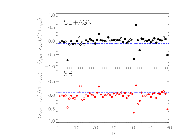
Figure 6: Comparison of the photometric redshift accuracy achieved by fitting the infrared spectrum of the sources listed in Table 2 with 2 SED components (i.e. starburst + AGN; upper panel) and with the starburst templates alone (lower panel). The meaning of the lines is the same as in Fig. 5.

We note that the estimated 99$\%$ error on the photometric redshift is particularly large for few sources lying in the redshift range $0.8\,\lower 2.0pt\hbox{${<\atop\hbox{\raise 4.0pt\hbox{$\sim$}}}$}\,z_{\rm spec}\,\lower 2.0pt\hbox{${<\atop\hbox{\raise 4.0pt\hbox{$\sim$}}}$}\,1$, i.e. ID32, ID43, ID48, and ID56. This follows from the shape of the SED of these objects. For ID32, ID43 and ID48 the measured spectrum is close to a power law for $\lambda\,\lower 2.0pt\hbox{${>\atop\hbox{\raise 4.0pt\hbox{$\sim$}}}$}\,8\mu$m, and this induces a degeneracy between the redshift and the normalization of the AGN sed component ($f_{2}$) around the minimum value of the $\chi^{2}$. The case of ID56 is more peculiar. At the redshift of the source (i.e. $z_{\rm spec}=1.017$), the rest-frame 9.7$\,\mu$m silicate absorption enters the AKARI 18$\,\mu$m filters, which is the broadest among the AKARI filters (FWHM$\sim$10$\,\mu$m); as a consequence the measured SED appears relatively flat between $15$ and $24\,\mu$m. However, while for objects like ID21, ID30, ID36, ID45, ID46 (all at $z=1$), a hint of the silicate absorption at $18\,\mu$m is still visible, in the case of ID56 the SED is featureless above 15$\,\mu$m. Consequently, the observed spectrum can be still reasonably well fitted by a mixture of starburst and AGN emission in a large redshift interval around $z\sim 1$.

According to our SED fitting results, sources with $P_{\chi^{2}}>1\%$ and $|\delta z|/(1+z_{\rm spec})\sim 10\%$ manifest different levels of AGN emission in their SED. In same cases the SED is well described by a starburst template (e.g. ID17, ID35, ID38), while in other cases an underlying AGN activity is found to contribute to the measured fluxes either at all wavebands (e.g. ID24, ID42, ID48, ID52, ID58) or only at longest wavelengths, i.e. 18 and 24$\,\mu$m (e.g. ID3, ID16). There are also some very peculiar/interesting cases of sources at $z_{\rm spec}\sim 1$ for which the flux above $\lambda\sim 10\,\mu$m is completely or significantly accounted for by the emission from an edge-on viewed dusty torus (e.g. ID21, ID27, ID30, ID39, ID46).

It is worth noticing that our SED-fitting procedure is meant to combine the SB and AGN SED components in such a way to minimize the value of the $\chi^{2}$ in Eq. 2 and not to maximize the probability associated to the minimum value of the $\chi^{2}$. In fact, while the value of $P_{\chi^{2}}$ depends on the number of degree of freedom of the problem (and on the assumption that the quantity in Eq. 2 follows exactly a $\chi^{2}$-distribution), that of the minimum $\chi^{2}$ does not. Consequently, there may be some sources for which the best fit to their SED gives a smaller value for $P_{\chi^{2}}$ when the fit is performed by setting a priori $f_{2}$ to zero than when both $f_{1}$ and $f_{2}$ are taken as free parameters, even if the resulting minimum $\chi^{2}$ is smaller in the latter case. In Table 3 we show, for comparison, the minimum reduced $\chi^{2}$ and the associated probability $P_{\chi^{2}}$ obtained when the measured SED is fitted with the starburst templates alone.
We note that there are several cases for which the value of $P_{\chi^{2}}$ is slightly lowered when using two SED components and in two cases it drops below the $1\%$ limit (ID39, ID40). On the other hand, accounting for an AGN component improves the goodness of the fit for many other objects in the sample, particularly when the measured SED is close to a power-law (see e.g. ID5, ID41 and ID48). However, for these extreme cases, a better fit doesn’t imply a better redshift accuracy which instead remains quite poor. In Fig. 6 we compare the photometric redshift accuracy, $(z_{\rm phot}-z_{\rm spec})/(1+z_{\rm spec})$, achieved by our two-SED fitting procedure (upper panel) with that obtained by fitting the observed SED with the starburst templates alone (lower panel). In both panels filled circles mark the sources with $P_{\chi^{2}}>1\%$ while open circles indicate sources with $P_{\chi^{2}}<1\%$. There are few cases in which, the redshift of the source is better recovered when accounting for an AGN component: ID24, ID29, ID43, however, we do not see on average a significant difference in the achieved redshift accuracy between the two-SED fitting approach and that based on the starburst templates alone.

For comparison, we also show in Fig 4 the result of the best-fit obtained when $f_{2}=0$. There are some sources, mainly at redshift $z\,\lower 2.0pt\hbox{${<\atop\hbox{\raise 4.0pt\hbox{$\sim$}}}$}\,0.5$, e.g. ID1, ID2, ID4, ID12, ID13, ID47 and ID57, for which the fit to the SED is very poor (i.e. $P_{\chi^{2}}\ll 1\%$) independently on the adopted SED fitting approach. Failure in reproducing the infrared spectrum of these sources could be due to an underestimate of the fluxes at 11 and 18$\,\mu$m. In fact, AKARI photometry were obtained under the assumption of point sources (see Pearson et al. 2008 for details), while most of the objects listed above are significantly extended in optical images (see Fig. 2). Moreover, ID1 and ID47 appear to be elliptical galaxies whose spectrum is not expected to be well-recovered by the starburst SED templates exploited here.

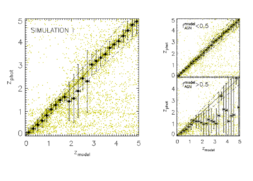
Figure 7: Simulation of photometric redshift accuracy with the AKARI NEP Deep Survey. The simulated spectra have been derived from the same models used for constructing the reference SED templates, i.e. Takagi et al. (2003, 2004) for the starburst and Efstathiou $\&$ Rowan-Robinson (1995) for the AGN. The filled circles with error bars are the mean value and the 1$\sigma$ dispersion provided by the Gaussian fit to the histogram of the $z_{\rm phot}$ values in intervals of 0.2 in $z_{\rm model}$. Only simulated spectra for which $P_{\chi^{2}}>1\%$ are taken into account (4919 over 5000). The dot-dashed lines delimit the region where $(z_{\rm phot}-z_{\rm model})/(1+z_{\rm model})<10\%$, while the solid line corresponds to the case $z_{\rm phot}=z_{\rm model}$. The photometric redshift accuracy achieved for the whole sample is shown in the left-hand panel while that derived for the subsamples of spectra with $f_{\rm AGN}^{\rm model}<0.5$ and $f_{\rm AGN}^{\rm model}>0.5$ is shown in the right-hand panels.

Table 4: 5$\sigma$ flux limits for the AKARI NEP-Deep Survey used in the simulations (from Wada et al. 2008).

$\lambda_{c}$ ($\mu$m)	2.43	3.16	4.14	7.3	9.1	10.7	15.7	18.3	23.0
Slim (mJy)	14.2	11.0	8.0	48.9	58.5	70.9	117.0	121.4	275.8

5 Simulations of the AKARI NEP Deep Survey

In order to investigate the photometric redshift accuracy achievable with the AKARI NEP Deep Survey we have generated three different sets of 5000 simulated spectra, including contributions from both starburst and AGN.

In all the simulations, which are described in the next subsections, the derived starburst and AGN components are linearly combined together with a relative contribution to the bolometric luminosity randomly selected between 0 and 1. Redshifts are randomly assigned in the range 0-5, assuming a uniform distribution, and the spectra are then normalized to the 24$\,\mu$m fluxes generated from the source count model of Lagache et al. (2003). A minimum 24$\,\mu$m flux of 100$\,\mu$Jy is assumed. The spectra are then convolved with the nine AKARI/IRC filters, spanning the wavelength range 2-24$\,\mu$m (they are shown in Fig. 1). We require the simulated spectra to be detected in at least five of the observed bands, according to the adopted 5$\sigma$ detection limits shown in Table 4 (from Wada et al. 2008). The corresponding 1$\sigma$ limits are used to introduce Gaussian fluctuations on the simulated fluxes and are adopted as the estimated error on the resulting fluxes. When a simulated spectrum is undetected at a certain waveband than both its flux and the accompanying error are set equal to half the 5$\sigma$ detection limit at that waveband.

For all the three sets of simulations, the resulting fluxes are fitted using the reference SED templates presented in subsection 2.3. A description of the SED models used to build the simulations and of the derived photometric accuracy is provided in the following subsections.

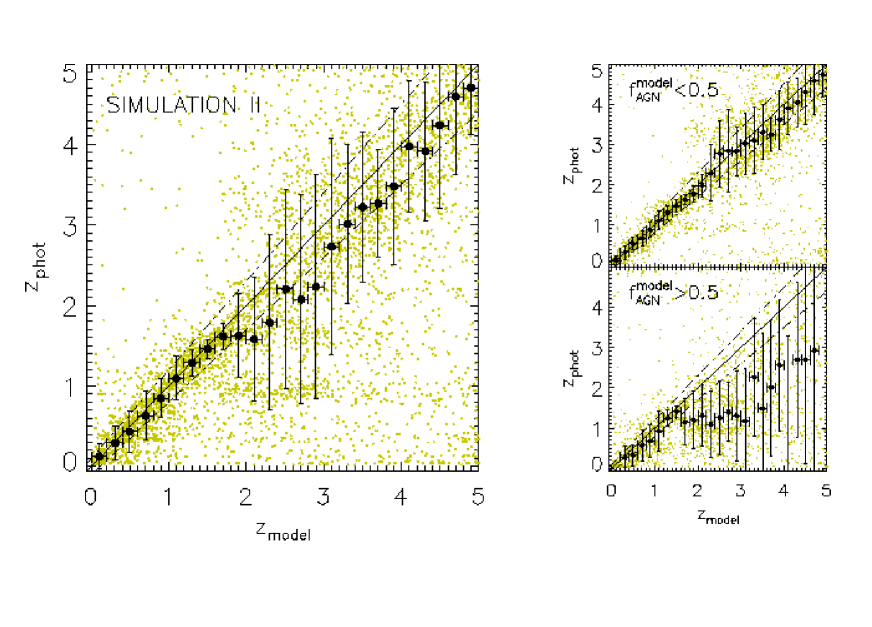
Figure 8: Photometric redshift accuracy with the AKARI NEP Deep Survey derived from the set of simulated spectra generated using the models of Efstathiou et al. (2000, 2003) and of Efstathiou $\&$ Rowan-Robinson (1995) for the starburst/cirrus and AGN infrared emissions, respectively. The meaning of the symbols and of the lines is the same as in Fig. 7. For 4859 simulated spectra (out of 5000) the fit has provided $P_{\chi^{2}}>1\%$.

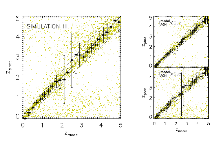
Figure 9: Photometric redshift accuracy with the AKARI NEP Deep Survey derived for the set of simulated spectra generated using the SWIRE SED templates. The meaning of the symbols and of the lines is the same as in Fig. 7. The simulated spectra for which the fit has provided $P_{\chi^{2}}>1\%$ are 4060 out of 5000.

5.1 Simulation I

The first set of simulated flux measurements (5000 spectra in total) have been obtained from the same SED models used to construct the reference SED templates, i.e. TAH03 model for the starburst and ER95 for the AGN. Each SED component is derived by randomly selecting the values of the SED parameters within the intervals specified in subsection 2.3.

The derived photometric redshifts, $z_{\rm phot}$, versus the simulated redshifts, $z_{\rm model}$, are shown in the left-hand panel of Fig. 7 where the filled circles with error bars represent the mean value and the 1$\sigma$ dispersion obtained by fitting a Gaussian to the histogram of the $z_{\rm phot}$ values in intervals of 0.2 in $z_{\rm model}$. Only simulated spectra with $P_{\chi^{2}}>1\%$ have been taken into account (they are represented by the small dots in the same figure). On average, the accuracy achievable on ($1+z$) is close to 10$\%$ (a limit indicated by the dot-dashed lines in the same figure) below $z\sim 2$ and above $z\sim 3$, while in the redshift interval $1.8\,\lower 2.0pt\hbox{${<\atop\hbox{\raise 4.0pt\hbox{$\sim$}}}$}\,z\,\lower 2.0pt\hbox{${<\atop\hbox{\raise 4.0pt\hbox{$\sim$}}}$}\,2.8$ the dispersion on the photo-$z$ estimates is particularly high. This behavior is mainly due to a significant number of points lying below the 10$\%$-accuracy region. Interestingly, we found that these data correspond to spectra with a dominant AGN component, and therefore with almost featureless power-law shape. To prove this we have splitted the whole set of simulated spectra into two subsamples according to the input value of the AGN fraction, i.e. $f_{\rm AGN}^{\rm model}<0.5$ and $f_{\rm AGN}^{\rm model}>0.5$ and calculated the photometric accuracy for each subsample. The results are presented in the right-hand panels of Fig. 7. Power-law like spectra have photometric redshifts which are systematically and significantly lower than the input redshifts. Once they are removed from the sample the achieved accuracy on $(1+z)$ gets close to 10$\%$ over the whole range of redshifts probed by the simulation.

5.2 Simulation II

The second set of 5000 simulated spectra has been constructed using the model of Efstathiou et al. (2000, hereafter ERS00) for the starburst emission while the AGN component has been modelled using the prescription of ER95, as done before. We have also included a third SED component describing the emission from the diffuse interstellar dust heated by old stars and/or quiescent star formation (infrared cirrus), for which we have followed the model of Efstathiou $\&$ Rowan-Robinson (2003, hereafter ER03).

According to ERS00 stars form primarily within optically thick giant molecular clouds (GMCs) and their model provides prescriptions for the evolution of the GMCs owing to the ionization-induced expansion of the HII regions. The evolution of the stellar population within the GMC is accounted for by using the Bruzual $\&$ Charlot (1993) stellar population synthesis models with a Salpeter Initial Mass Function (IMF) and a star mass range of 0.1-125 M_⊙. The absorption/emission properties of the dust within the GMCs are derived according to the model of Siebenmorgen $\&$ Krugel (1992) which assume three different populations of dust grains: large grains, small graphite particles and PAHs. Starburst galaxies are treated as an ensemble of GMCs at different evolutionary stages. The star formation rate is modeled with an exponential functional form $\dot{M}\propto e^{-t/\tau_{\rm SB}}$. Here we set the e-folding time of the star-formation rate, $\tau_{\rm SB}$, to 20 Myr while the age of the HII region phase, Age_SB, and the initial optical depth of GMCs, $\tau_{0}$, are treated as free parameters, with Age${}_{\rm SB}=0-72$ Myr and $\tau_{0}=50-200$.

Figure 10: Upper panel: photometric redshift accuracy, $\delta z/(1+z_{\rm model})$, as a function of the input value of the AGN fraction, $f_{\rm AGN}^{\rm model}$, derived from the three sets of simulations presented here. The filled circles with error bars are the mean value and the 1$\sigma$ dispersion provided by the Gaussian fit to the histogram of the $\delta z/(1+z_{\rm model})$ values in intervals of 0.2 in $f_{\rm AGN}^{\rm model}$. Only spectra with $P_{\chi^{2}}>1\%$ have been taken into account. Lower panels: corresponding accuracy achieved on the AGN fraction. Again, the filled circles with error bars are the mean value and the 1$\sigma$ dispersion provided by the Gaussian fit to the histogram of the $(f_{\rm AGN}^{\rm fit}-f_{\rm AGN}^{\rm model})/f_{\rm AGN}^{\rm model}$ values in intervals of 0.2 in $f_{\rm AGN}^{\rm model}$.

The infrared cirrus is characterized by lower optical depth and lower temperatures of the dust ( ${<\atop\hbox{\raise 4.0pt\hbox{$\sim$}}}$  30 K), compared to what occurs in starburst regions. However, as in ERS00, stars are assumed to have formed within GMCs but their evolution is followed well beyond the complete dispersion of the GMCs (i.e. after $\sim 72$ Myr), when the starlight can be absorbed only by the general interstellar medium. The input stellar radiation field is computed from the stellar population synthesis model of Bruzual $\&$ Charlot (1993) while the grain model of Siebenmorgen $\&$ Krugel (1992) is used again to derive the absorption/emission properties of the dust. The extinction parameter $A_{V}$ regulates the proportion of the UV to near-IR light that is absorbed by the ISM and re-emitted in the far-IR and sub-mm bands. The temperature of the interstellar dust is determined by the intensity of the radiation field. ER03 characterize this in terms of the ratio $\Phi$ of the bolometric intensity of the radiation field to that in the stellar radiation field in the solar neighborhood. Since the value of $\Phi$ influences only the far-infrared shape of the SED, i.e. the position of the peak of the SED (the higher $\Phi$, the hotter the dust and the lower the wavelength of the peak), the exact choice of its value is not relevant for our purpose and therefore we just set it to 1. Before the complete evaporation of the GMC, the non-spherical evolution of the molecular cocoon may allow a fraction $f$ of the starlight to escape without any dust absorption from the GMC. Here we set $f=1$ after 3 Myr as in ER03. The age of the cirrus component, Age_CIR, and the e-folding time of the star-formation rate, $\tau_{\rm CIR}$, are treated as free parameters and varied consistently with the redshift of the source (i.e. always assuring that Age_CIR and $\tau_{\rm CIR}$ are lower than the age of the Universe at the redshift of the source). The visual extinction is chosen within the range $A_{V}=0-3$.

Each simulated SED component, i.e. starburst, cirrus and AGN, is derived by randomly selecting the values of the SED parameters within the intervals mentioned before. The fractions of the bolometric luminosity contributed by the AGN and by the starburst+cirrus are selected at random between 0 and 1. The contribution from the starburst+cirrus is then randomly divided between the two components (i.e. starburst and cirrus); in this way we guarantee that the final sample of simulated spectra include almost 50$\%$ of AGN dominated SED, as in the previous sample.

The results on the photometric redshift accuracy are shown in Fig. 8, where the meaning of the symbols and of the lines is the same as in Fig. 7. The achieved accuracy on $(1+z)$ is close to $10\%$ below $z\sim 1.8$ but decreases significantly above $z\sim 2$, particularly in the interval $z\sim 2-3$. Although AGN power-law like spectra are found to be responsible for the significant fraction of data points lying below the $10\%$-accuracy region (see right-hand panels in the same figure), this effect alone does not account for the relatively low accuracy achieved in the interval $2\,\lower 2.0pt\hbox{${<\atop\hbox{\raise 4.0pt\hbox{$\sim$}}}$}\,z\,\lower 2.0pt\hbox{${<\atop\hbox{\raise 4.0pt\hbox{$\sim$}}}$}\,3$. In this redshift range the only valuable redshift indicators are the 1.6$\,\mu$m bump and the PAH 3.3$\,\mu$m emission feature. The simulated spectra including a cirrus component are more challenging for our reference SED templates to reproduce. In fact the latter are meant for fitting relatively young starburst galaxies only, with (eventually) an additional AGN component. It is also worth noting that for $2\,\lower 2.0pt\hbox{${<\atop\hbox{\raise 4.0pt\hbox{$\sim$}}}$}\,z\,\lower 2.0pt\hbox{${<\atop\hbox{\raise 4.0pt\hbox{$\sim$}}}$}\,3$ the 1.6$\,\mu$m bump is shifted to wavelengths $4.8\,\lower 2.0pt\hbox{${<\atop\hbox{\raise 4.0pt\hbox{$\sim$}}}$}\,\lambda\,\lower 2.0pt\hbox{${<\atop\hbox{\raise 4.0pt\hbox{$\sim$}}}$}\,6.4$, where the AKARI coverage is quite poor (see Fig. 1). This contributes to the observed decrease in the photo-z accuracy in that redshift interval.

5.3 Simulation III

The third simulation is built from the empirical spectra used to fit the SED of different types of sources in the Spitzer Wide-Area Infrared Extragalactic(SWIRE) survey (see Polletta et al. 2008 and references therein). The SWIRE template library contains 25 templates: 3 ellipticals, 7 spirals, 6 starbursts, 7 AGNs (3 type 1 AGNs, 4 type 2 AGNs), and 2 composite (starburst+AGN). The elliptical, spiral and starburst templates were generated using the the GRASIL code (Silva et al. 1998). The ellipticals correspond to three different ages: 2 ,5 and 13 bilion years. The 7 spirals range from early to late types (S0-Sdm). The starburst templates correspond to the SEDs of NGC6090, NGC6240, M82, Arp220, IRAS22491-1808, and IRAS20551-4250. In all of the spirals and starburst templates the spectral region between 5 and 12$\,\mu$m, where PAH broad emission and silicate absorption features are observed, was replaced using observed infrared spectra from the PHT-S spectrometer on the ISO and from IRS on Spitzer.

AGN templates corresponding to Seyfert 1.8 and Seyfert 2 galaxies were obtained by combining models, broadband photometric data (NED) and ISO PHT-S spectra of a random sample of 28 Seyfert galaxies. Three other AGN templates represent optically selected QSOs with different values of infrared/optical flux ratios, derived by combining the Sloan Digital Sky Survey (SDSS) quasar composite spectrum and rest-frame IR data of a sample of 35 SDSS/SWIRE quasars and then assuming three different IR SEDs. Of the remaining AGN templates (type 2 QSOs) one was obtained by combining the observed optical/near-IR spectrum of the red quasar FIRST J013435.7-093102 and the rest-frame IR data from the quasars in the Palomar-Green sample with consistent optical SEDs. The other type 2 QSO template corresponds to the model used to fit the SED of a heavily obscured type 2 QSO, SWIRE$\underline{~{}}$J104409.95+585224.8 (Polletta et al. 2006)

The composite (AGN+SB) templates are empirical templates created to fit the SEDs of the heavily obscured BAL QSO Mrk 231 (Berta 2005) and the Seyfert 2 galaxy IRAS 19254-7245 South (Berta et al. 2003). They both contain a powerful starburst component, responsible for their large infrared luminosities, and an AGN component that contributes to the mid-IR luminosities.

Elliptical, spirals, starburst and AGN+SB templates were randomly selected within the available sample. If the SED did not already include an AGN component (i.e. it was not one of the two SWIRE composite spectra) than an AGN templates was chosen at random from the SWIRE sample and added to the SED, with a relative contribution to the bolometric luminosity randomly selected from a uniform distribution between 0 and 1.

The results of the photometric redshift accuracy are presented in Fig. 9. Again we observe a large scatter in the photo-z estimates in the interval $2\,\lower 2.0pt\hbox{${<\atop\hbox{\raise 4.0pt\hbox{$\sim$}}}$}\,z\,\lower 2.0pt\hbox{${<\atop\hbox{\raise 4.0pt\hbox{$\sim$}}}$}\,3$ where the main infrared features are shifted outside the range of wavelengths covered by AKARI and the 1.6$\,\mu$m feature is not well sampled because of the lack of coverage around $\lambda\sim 5-6\,\mu$m. Despite this, the accuracy achieved on $(1+z)$ is better than 10$\%$ up to $z=5$.

5.4 Discussion

Figure 11: Example of a simulated SED with a dominant AGN component ($f_{\rm AGN}^{\rm model}>0.8$) for which the best-fit provides low AGN fraction ($f_{\rm AGN}^{\rm fit}<0.2$). The input SED model is shown in the upper panel: the solid line is the total SED and includes contributions from a starburst (dashed line) and an AGN (dot-dashed), as derived from the models of Takagi et al. (2003) and Efsathiou $\&$ Rowan-Robinson (1995), respectively. The SED best-fit is shown in the lower panel. The meaning of the lines is the same as above.

The results of the simulations suggest that for $z_{\rm model}\,\lower 2.0pt\hbox{${<\atop\hbox{\raise 4.0pt\hbox{$\sim$}}}$}\,1.8$, i.e. when the photo-$z$ estimate is based on the passage of the PAH features through the AKARI filters, the achieved accuracy on redshift does not depend significantly on the precise details of the underlying starburst model and the estimated redshift can be considered reliable, irrespective of the AGN fraction. At higher redshifts instead, featureless AGN-dominated spectra make the recovery of redshift extremely challenging from infrared data alone. The effect of the AGN infrared emission on the photo-$z$ accuracy is made even clearer in the top panels of Fig. 10 where the quantity $(z_{\rm phot}-z_{\rm model})/(1+z_{\rm model})$ is shown as a function of the input value of the AGN fraction for the three sets of simulations presented here. The dispersion on ($1+z$) increases from $\,\lower 2.0pt\hbox{${<\atop\hbox{\raise 4.0pt\hbox{$\sim$}}}$}\,10\%$ to $\,\lower 2.0pt\hbox{${>\atop\hbox{\raise 4.0pt\hbox{$\sim$}}}$}\,30\%$ as the AGN fraction passes from 0.1 to 0.5, while for $f_{\rm AGN}^{\rm model}\,\lower 2.0pt\hbox{${>\atop\hbox{\raise 4.0pt\hbox{$\sim$}}}$}\,0.5$ the photometric estimate of the redshift becomes totaly unreliable, at least according to the results based on the first two sets of simulations. On the other hand, the recovery of the AGN fraction itself becomes very challenging when $f_{\rm AGN}^{\rm model}\,\lower 2.0pt\hbox{${>\atop\hbox{\raise 4.0pt\hbox{$\sim$}}}$}\,0.2$ as demonstrated in the lower panel of the same figure. An example of such a case is shown in Fig. 11.

These results indicates that infrared data alone are a valuable tool for redshift estimate but they are not very efficient in constraining the AGN fraction, at least when the infrared SED is AGN dominated. In such cases the support of data at other wavelengths (e.g. optical and near-infrared, radio, X-ray) is needed to recover the real nature of the infrared emission.

We note however that AGN power-law like spectra can be easily singling out by fitting a line to the observed $\log S-\log\lambda$ diagram ($S$ being the measured flux and $\lambda$ the observing wavelength) and analyzing the probability associated to the corresponding $\chi^{2}$, $P_{\chi^{2}}^{\rm pl}$. In Fig. 12 we show the photometric redshift accuracy achieved in the three sets of simulations after dividing the spectra into those with $P_{\chi^{2}}^{\rm pl}>1\%$ (i.e. power-law shape) and those with $P_{\chi^{2}}^{\rm pl}<1\%$. In all cases, the criterion of selection of the SED based on fitting a line to the observed $\log S-\log\lambda$ diagram acts exactly in the same way as the one relying on the input value of the AGN fraction (see right-hand panels of Figs 7 to 9). Therefore we suggest the following rules as a practical guideline for interpreting photometric redshifts in AKARI NEP Deep Survey when using the methods illustrated here: if the observed spectrum is poorly described by a power-law than the photometric redshift can be considered accurate up to $z_{\rm phot}\sim 5$. When instead the observed spectrum is very close to a power-law, it is high probable that the redshift of the source has been significantly underestimated and it should be rejected.

Figure 12: Simulated photometric redshift accuracy with the AKARI NEP Deep Survey for power-law like spectra ($P_{\chi^{2}}^{\rm pl}>1\%$, bottom panels) and for spectra which are poorly fitted by a power-law ($P_{\chi^{2}}^{\rm pl}<1\%$, top panels). The panels refers from left to right to simulations based on the Takagi et al. (2003) model for the starbursts, the Efstathiou et al. (2000, 2003) models for the starburst/cirrus and the SWIRE sed templates (Polletta et al. 2008).

6 Conclusions

We have tested the reliability of the photometric redshift estimates based on infrared photometry alone on a sample of 59 galaxies with spectroscopic redshifts $0.5\,\lower 2.0pt\hbox{${<\atop\hbox{\raise 4.0pt\hbox{$\sim$}}}$}\,z_{\rm spec}\,\lower 2.0pt\hbox{${<\atop\hbox{\raise 4.0pt\hbox{$\sim$}}}$}\,1.5$ drawn from the GOODS-N field, combining together infrared data from literature (i.e. Spitzer and ISO) and new AKARI 11 and 18$\,\mu$m photometric data. Our SED fitting procedure allows for the contribution to the infrared emission from both starburst and AGN, described according to the models of Takagi et al. (2003) and Efstathiou $\&$ Rowan-Robinson (1995), respectively. Three different sets of simulations derived from both theoretical SED models and empirical spectra have been used to tested the photo-z accuracy achievable with the AKARI NEP Deep Survey.
The main conclusions are summarized as follows.

• The SEDs of 42 out of our 59 sources are well fitted (i.e. $P_{\chi^{2}}>1\%$) by our starburst+AGN SED reference templates. For all the sources in the sample bar 7 the achieved accuracy on $(1+z)$ is close to or better than $10\%$. Even in the case of a “bad” fit (i.e. $P_{\chi^{2}}<1\%$) the mean features in the spectrum are recognized and the redshift is still reasonably well recovered. Sources at $z\,\lower 2.0pt\hbox{${>\atop\hbox{\raise 4.0pt\hbox{$\sim$}}}$}\,2$ (three in total) display in general a power-law infrared spectrum, whose lack of any evident feature make the estimate of redshift quite difficult on the basis of infrared data alone. In such cases data at longer wavelengths, near or beyond the peak associated to the dust emission or at decimetric radio wavelengths, are needed to remove the degeneracies in redshifts.

• Simulations show that the infrared data alone produced by the AKARI NEP Deep Survey will provide photometric redshifts with a typical accuracy of $|z_{\rm phot}-z_{\rm spec}|/(1+z_{\rm spec})\sim 10\%$ (1$\,\sigma$) at $z\,\lower 2.0pt\hbox{${<\atop\hbox{\raise 4.0pt\hbox{$\sim$}}}$}\,2$, in agreement with our findings for the spectroscopic sample. At higher redshifts the PAH features are shifted outside the wavelength range covered by AKARI and the 1.6$\,\mu$m stellar bump is then exploited as a redshift indicator; the accuracy achievable in this case on $(1+z)$ is $\sim 10-15\%$, provided that the AGN contribution to the infrared emission is subdominant.

  Although our reference SED templates allow for an AGN contribution to the infrared emission, the AGN fraction is poorly constrained when the SED is AGN dominated and therefore does not exhibit any evident features. In these cases the support of photometric data at other wavelengths (e.g. X-ray, submillimeter or decimeter radio wavelengths) can help to better constrain the relative contributions of starburst and AGN to the observed SED.

References

- [1] Adelberger K. L., Steidel C. C., Shapley A. E., Hunt M. P., Erb D. K., Reddy N. A., Pettini M., 2004, ApJ, 607, 226
- [2] Arimoto N., Yoshii Y., Takahara F., 1992, AA, 253, 21
- [3] Avni Y., 1976, ApJ, 210, 642
- [4] Aussel H. Cesarsky C.J., Elbaz D., Starck J.L., 1999, ApJ, 342, 313
- [5] Berta S. 2005, Ph.D. thesis, Univ. Padua
- [6] Berta S., Fritz J., Francescini A., Bressan A., Pernechele C., 2003, AA, 403, 119
- [7] Bertin E. Arnouts S., 1996, AAS, 117, 393
- [8] Bolzonella M., Miralles J.-M., Pello R., 2000, AA, 363, 476
- [9] Bruzual A. Charlot S., 1993, ApJ, 405, 538
- [10] Capak P. et al. 2004, AJ, 127, 180
- [11] Cowie L.L., Barger A.J., Hu E.M., Capak P., Songaila, A, 2004, AJ, 127, 3137
- [12] Chapman S. C., Blain A. W., Smail I., Ivison R. J., 2005, ApJ, 622, 772
- [13] Chapman, S. C., Smail I., Windhorst R., Muxlow T., Ivison R. J., 2004, ApJ, 611, 732
- [14] Dickinson M. et al., 2001, BAAS, 33, 820
- [15] Efstathiou A. Rowan-Robinson M., 1995, MNRAS, 273, 649 (ER95)
- [16] Efstathiou A. Rowan-Robinson M., 2003, MNRAS, 343, 322 (ER03)
- [17] Efstathiou A., Rowan-Robinson M. Siebenmorgen R., 2000, MNRAS, 313, 734 (ERS00)
- [18] Farrah D., Lonsdale C.J., Weedman D.W., Spoon H.W.W., Rowan-Robinson M., Polletta M., Oliver S., Houck J.R., Smith H.E., 2008, ApJ, 677, 957
- [19] Giacconi R. et al. 2000, AAS, 197, 9001
- [20] Hughes D.H. et al. 1998, Nature, 394, 241
- [21] Kessler M.F. et al. 1996, AA, 315, L27
- [22] Kodawa T., Arimoto N., 1997, AA, 320, 41
- [23] Lagache G., Puget J.-L., Dole H., 2005, ARAA, 43, 727
- [24] Lagache G., Dole H., Puget J.-L., 2003, MNRAS, 338, 555
- [25] Lee H. M. et al. 2008, PASJ, submitted
- [26] Oke J.B., et al. 1995, PASP, 107, 375
- [27] Pearson C. et al. 2008, in preparation
- [28] Polletta M. et al. 2006, ApJ, 642, 673
- [29] Polletta M. et al. 2008, ApJ, 663, 81
- [30] Reddy N. A., Steidel C. C., Erb D. K., Shapley A. E., Pettini M., 2006, ApJ, 653, 1004
- [31] Rowan-Robinson M., 1992, MNRAS, 258, 787
- [32] Sawicki M., 2002, AJ, 124, 3050
- [33] Serjeant S. et al., 2003, MNRAS, 344, 887
- [34] Siebenmorgen R., Krugel E., 1992, AA, 259, 614
- [35] Silva L., Granato G.L., Bressan A. Danese L., 1998, ApJ, 509, 103
- [36] Steidel C. C., Adelberger K. L., Shapley A. E., Pettini M., Dickinson M., Giavalisco M., 2003, ApJ, 592, 728
- [37] Steidel C. C., Shapley A. E., Pettini M., Adelberger K. L., Erb D. K., Reddy N. A., Hunt M. P., 2004, ApJ, 604, 534
- [38] Takagi T., Arimoto N., Hanami H., 2003, MNRAS, 340, 813 (TAH03)
- [39] Takagi T., Hanami H., Arimoto N., 2004, MNRAS, 355, 424 (THA04)
- [40] Takagi T. C. P. Pearson, 2005, MNRAS, 357, 165
- [41] Takagi T. et al. 2007, PASJ, 59, 557
- [42] Teplitz H.I., Charmandaris V., Chary R., Colbert J.W., Armus L., Weedman D., 2005, ApJ, 634, 128
- [43] Wada T. et al. 2008, PASJ in press
- [44] Williams R.E. et al. 1996, AJ, 112, 1335
- [45] Wirth G.D. et al., 2004, AJ, 127, 3121