Diffraction from the $\beta$-sheet crystallites in spider silk

Abstract

We analyze the wide angle x-ray scattering from oriented spider silk fibers in terms of a quantitative scattering model, including both structural and statistical parameters of the $\beta$-sheet crystallites of spider silk in the amorphous matrix. The model is based on kinematic scattering theory and allows for rather general correlations of the positional and orientational degrees of freedom, including the crystallite’s size, composition and dimension of the unit cell. The model is evaluated numerically and compared to experimental scattering intensities allowing us to extract the geometric and statistical parameters. We show explicitly that for the experimentally found mosaicity (width of the orientational distribution) inter-crystallite effects are negligible and the data can be analyzed in terms of single crystallite scattering, as is usually assumed in the literature.

1 Introduction

Spider silk is a material which is since long known to everybody, but which only more recently receives great appreciation by the scientific community for its outstanding material properties grubb97 ; properties . Interest here has focused on the so-called dragline fiber, the high strength fibers which orb web spiders produce from essentially only two proteins to build their net’s frame and radii, and also to support their own body weight after an intentional fall down during escape. Evolution has optimized dragline fibers for tensile strength, extensibility and energy dissipation. Dragline silk can support relatively large strains and has a tensile strength comparable to steel or Kevlar. For the energy density which can be dissipated in the material before breaking, the so-called tenacy (toughness), values of $160\,{\rm MJ/m^{3}}$ have been reported gosline ; silkpolymers , e.g. for different Nephila species, on which most studies have been carried out. An understanding of the structural origins of these mechanical properties is of fundamental interest, and may at the same time serve the development of biomimetic material design scheibel2004 ; scheibel2006 , using recombinant and synthetic approaches ScheibelAPA ; KaplanAPA ; BauschAPA . As for other biomaterials, the correlation between structure and the mechanical properties can only be clarified by advanced structural characterization accompanied by numerical modelling. To this end, not only the mechanical properties VollrathAPA ; ZbilutAPA resulting from the structure, but also the structure itself has to be modelled to exploit and to interpret the experimental data. Such efforts have in the past led to a quantitative understanding of many biomaterials like bone, tendons and wood fratzl1 ; fratzl2 .

As deduced from x-ray scattering warwicker ; grubb97 ; becker ; grubb_jelinski1 and NMR experiments nmr , spider silks are characterized by a seemingly rather simple design: the alanine-rich segments of the fibroin polypeptide chain fold into $\beta$-sheet nano-crystallites (similar to poly-L-alanine crystals) embedded in an amorphous network of chains (containing predominately glycine). The crystalline component makes up an estimated 20%-30% of the total volume, and may represent cross-links in the polymer network, interconnecting several different chains. At the same time the detailed investigation of the structure is complicated, at least on the single fiber level, by the relatively small diameters in the range of $1-10\,{\rm\mu m}$, depending on the species. Using highly brilliant microfocused synchrotron radiation, diffraction patterns can be obtained not only on thick samples of fiber bundles, but also on a single fiber vollrath1999 ; vollrath2000 ; vollrath2001 ; riekel99 ; vollrath2004 ; vollrath2005 . Single fiber diffraction was then used under simultaneous controlled mechanical load in order to investigate changes of the molecular structure with increasing strain up to failure Glisovic08 . Note that single fiber diffraction, where possible, is much better suited to correlate the structure to controlled mechanical load, since the strain distribution in bundles is intrinsically inhomogeneous, and the majority of load may be taken up by a small minority of fibers.

While progress of the experimental diffraction studies has been evident, the analysis of the data still relies on the classical classification and indexing scheme introduced by Warwicker. According to Warwicker, the $\beta$-sheet cristallites of the dragline of Nephila fall into the so-called system 3 of a nearly orthorhombic unit cell warwicker ; marsh with lattice constants $10.6\times 9.44\times 6.95$ Å warwicker . To fix the coordinate system, they define the $x$-axis to be in the direction of the amino acid side chains connecting different $\beta$-sheets with a lattice constant of $a_{x}=10.6$ Å  while the $y$-axis denotes the direction along the hydrogen bonds of the $\beta$-sheets with a lattice constant of $a_{y}=9.44$ Å. Finally the $z$-axis corresponds to the axis along the covalent peptide bonds (main chain) with a lattice constant $a_{z}=6.95$ Å. The $z$-axis with small lattice constant is well-aligned along the fiber axis. Note that while we follow this commen convention, other notations and choices of axis are also used in the literature. While helpful, the indexing scheme does not give any precise information on the exact structure of the unit cell, and on the fact whether the $\beta$-pleated sheets are composed of parallel or antiparallel strands, and how the two-dimensional sheets are arranged to stacks. To this end, not only peak positions but the entire rather broad intensity distribution has to be analyzed. To interpret the scattering image it is essential to know, whether correlations between different crystallites are important or whether the measured data can be accounted for by the scattering of single crystallites, averaged over fluctuating orientations. It is also not clear, whether correlations between translational and rotational degrees of freedom are important. Finally, the powder averaging taking into account the fiber symmetry experimental mosaicity (orientational distribution) must be quantitatively taken into account.

In this work we built a scattering model based on kinematic scattering theory and compare the numerically calculated scattering intensity with the experimental wide angle scattering distribution measured from aligned silk fibers. The numerical calculations allow for a quantitative comparison to the experimental data and yield both structural and statistical parameters. Note that the small size of crystallites, leading to correspondingly broad reflections, and a generally rather low number of external peaks exclude a standard crystallographic approach. The structural parameters concern the crystal structure, in particular the atomic positions in the unit cell, and the crystallite size. The composition is assumed to be that of ideal polyalanine without lattice defects. This assumption is partly justified by the fact that the small size of the crystallite is the ’dominating defect’ in this material. The statistical parameters relate to the orientational distribution of the crytallite symmetry axis with respect to the fiber axis and the correlations between crystallites. The model is constructed based on a quite general approach, allowing independently for correlations between center-of-mass positions (translations) and crystallite orientations (rotations).

The paper is organized as follows. In Sec. 2 we introduce the basic model with parameters for the crystallite size, lattice constants and statistical parameters for the crystallites’ position and orientation. Subsequently, in Sec. 3 we compute the scattering function for our model. Sec. 4 specifies the different atomic configurations which are conceivable for polyalanine. The main results and the comparison of calculated and measured intensities are presented in section 5, before the paper closes with a short conclusion.

2 Model

In this section we present a simple model of spider silk which allows us to compute the scattering function

$$G({\bf q})=\left\langle\left|\sum\nolimits_{j}f_{j}\exp(i{\bf q}{\bf r}_{j})\right|^{2}\right\rangle$$ (1)

as measured in X-ray scattering experiments. The atomic positions are denoted by ${\bf r}_{j}$ and the atomic form factors by $f_{j}$. The modeling proceeds on three different levels: 1) On the largest lengthscales spider silk is modelled as an ensemble of crystallites embedded in an amorphous matrix and preferentially oriented along the fiber axis. 2) Each crystallite is composed of parallel or antiparallel $\beta$-sheets. 3) Each unit cell contains a given number of amino acids, whose arrangements have been classified by Warwicker warwicker . In Fig. (1, bottom) we show an illustration of Bombyx mori by Geis Zubay .

In the following we shall build up a model, starting on the smallest scales and working up to the whole system. Subsequently we will compare our calculated scattering functions with experimental data. Thereby we are able to determine the arrangement of atoms in the unit cell which optimizes the agreement between model and experiment.

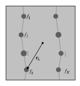
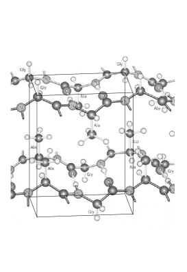
Figure 1: Top: Schematic view of the unit cell. Atom $k$ is loacted at position ${\bf r}_{k}$, and the atom type is specified by the form factor $f_{k}$ of the atom. For simplification schematic illustrations are in 2D, if possible, even though the model refers to three space dimensions, $D=3$. Bottom: Possible configuration inside the unit cell (illustration adapted from Zubay ).

2.1 Unit cell

One unit cell of a crystallite is described as a set of atoms at positions ${\bf r}_{k}$ relative to the center of the unit cell, where $k=1,2,...,K$ runs through the atoms of the unit cell (see Fig. 1, top panel, for a schematic drawing). Each atom is assigned a form factor $f_{k}$, specifying the scattering strength of the respective atom type.

2.2 Crystallite

A crystallite is composed of $M=M_{x}M_{y}M_{z}$ unit cells, replicated $M_{x}$, $M_{y}$ and $M_{z}$ times along the primitive vectors ${\bf a}_{x}$, ${\bf a}_{y}$ and ${\bf a}_{z}$, respectively. The unit cells in a crystallite are numbered by a vector index ${\bf m}=(m_{x},m_{y},m_{z})$, where $m_{\nu}=1,2,...,M_{\nu}$ for $\nu=x,y,z$. Hence the center of mass of unit cell ${\bf m}$ has position vector

$${\bf\tilde{s}}_{\bf m}=m_{x}{\bf a}_{x}+m_{y}{\bf a}_{y}+m_{z}{\bf a}_{z}.$$

Actually it is more convenient to measure all distances with respect to the center of the whole crystallite

$${\bf s}_{\rm cm}=\frac{(M_{x}+1){\bf a}_{x}+(M_{y}+1){\bf a}_{y}+(M_{z}+1){\bf a}_{z}}{2}$$

so that ${\bf{s}}_{\bf m}={\bf\tilde{s}}_{\bf m}-{\bf s}_{\rm cm}$ denotes the position of unit cell ${\bf m}$ relative to the center of the crytallite to which it belongs (see Fig. 2) and the position of atom $k$ in unit cell ${\bf m}$ relative to the center of the crystallite is

$${\bf r}_{{\bf m},k}={\bf s}_{\bf m}+{\bf r}_{k}$$ (2)

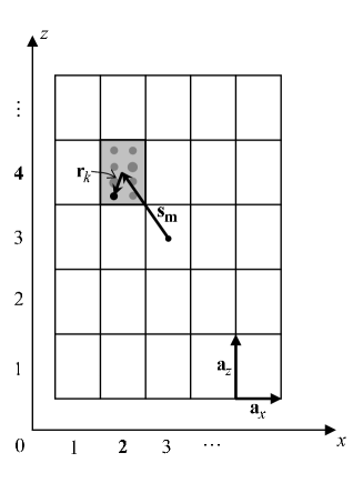
Figure 2: Schematic view of the crystallite. The vector ${\bf s}_{\bf m}$ goes from the center of the crystallite to the unit cell ${\bf m}$. From there ${\bf r}_{k}$ goes to atom $k$.

2.3 Ensemble of Crystallites

The whole system is composed of $N$ such crystallites at positions ${\bf R}^{(j)}$ with $j=1,2,...N$ (see Fig. 3). The crystallites are not perfectly aligned with the fiber axis, instead their orientation fluctuates. The orientation of a single crystallite is specified by three Euler angles $\phi^{(j)},\theta^{(j)},\psi^{(j)}$ (see Fig. 4, bottom). Here we have chosen the $z$-axis as the fiber axis and $\theta$ denotes the angle between the $z$-direction of the crystallites (direction of covalent bonds) and the fiber axis. The atomic positions of the rotated crystallite are obtained from the configuration which is perfectly aligned with the $z$-axis by applying a rotation matrix $\underline{\underline{D}}^{(j)}$ (see Fig. 4, top):

$${\bf r}_{{\bf m},k}^{(j)}={\bf R}^{(j)}+\underline{\underline{D}}^{(j)}{\bf r}_{{\bf m},k}\,.$$ (3)

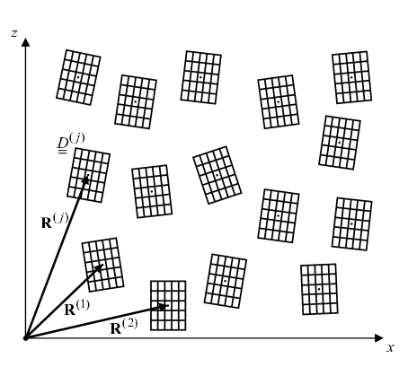
Figure 3: The whole system is composed of crystallites at positions ${\bf R}^{(j)}$. They can be rotated by rotation matrices $\underline{\underline{D}}^{(j)}$.

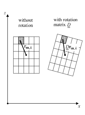
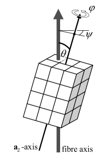
Figure 4: Top: The position of atom $k$ in unit cell ${\bf m}$ of the rotated crystallite is obtained by applying the rotation matrix $\underline{\underline{D}}{\bf r}_{{\bf m},k}$ to the position vector in the aligned configuration. Bottom: Illustration of Euler angles in 3D. The angle $\theta$ specifies the deviation of the crystallite’s ${\bf a}_{z}$-axis from the fiber axis of the strand. $\phi$ is the rotation of the crystallite about it’s own ${\bf a}_{z}$-axis, and $\psi$ is the rotation of the ${\bf a}_{z}$-axis about the fiber axis (after the $\theta$-rotation).

In the experiment the scattering intensity is obtained for a large system, consisting of many crystallites. Hence it is reasonable to assume that the scattering function is self-averaging and hence can be averaged over the positions and orientations of the crystallites. We use angular brackets $\langle\,\,\rangle$ to denote the average of an observable $\mathcal{O}$ over crystallite positions ${\bf R}^{(j)}$ and orientations $\underline{\underline{D}}^{(j)}$:

$$\left\langle\mathcal{O}\right\rangle=\int\prod_{j=1}^{N}\left(d^{3}{\!R}^{(j)}\mathcal{D}\underline{\underline{D}}^{(j)}\right)\,\mathcal{P}_{\rm pos}({\bf R}^{(1)},...,{\bf R}^{(N)})\mathcal{O}\,.$$ (4)

Here, the crystallite positions follow the distribution function $\mathcal{P}_{\rm pos}({\bf R}^{(1)},...,{\bf R}^{(N)})$ which in general includes correlations. In contrast the orientation of each crystallite is assumed to be independent of the others. The average over all orientations

$$\mathcal{D}\underline{\underline{D}}^{(j)}=d\phi^{(j)}d\theta^{(j)}d\psi^{(j)}\sin\theta^{(j)}\,\mathcal{P}_{\rm angle}(\phi^{(j)},\theta^{(j)},\psi^{(j)})$$ (5)

involves the angular distribution function $\mathcal{P}_{\rm angle}(\phi,\theta,\psi)$, which is the same for each crystallite. In the simplest model we assume a Gaussian distribution for the deviations of the crystallite axis from the fiber axis $\mathcal{P}_{\rm angle}(\phi,\theta,\psi)$ $\sim\exp(-\frac{\theta^{2}}{\theta_{0}^{2}})$ while all values of $\phi$ and $\psi$ between $0$ and $2\pi$ are equally likely.

2.4 Continuous background

The space between the crystallites is filled with water molecules and strands connecting the crystallites, which are called amorphous matrix. In the scope of this work, we are not interested in the details of its structure and model it as a continuous background density $\varrho_{0}$, chosen to match the average scattering density of the crystallite (see Fig. 5): $\varrho_{0}=\sum_{k=1}^{K}f_{k}/V_{\rm uc}$. Here $V_{\rm uc}$ is the volume of the unit cell. Inside the crystallite there is no background intensity which is achieved in our model by cutting out a spherical cavity, $V({\bf r})$, around each atom ${\bf r}={\bf r}_{{\bf m},k}^{(j)}$. For simplicity we assume a Gaussian cavity

$$V({\bf r})=\frac{\bar{f}}{(2\pi\xi^{2})^{3/2}}\exp\left(-\frac{{\bf r}^{2}}{2\xi^{2}}\right)\,.$$ (6)

and choose the amplitude such that the average density inside the crystallites is zero:

$$0=\int_{\rm crystallite}d^{3}r\left(\varrho_{0}-\sum_{{\bf m}}^{\bf M}\sum_{k=1}^{K}V({\bf r}-{\bf r}_{{\bf m},k})\right)\,,$$ (7)

where the sum over the vector index $\sum_{{\bf m}}^{\bf M}$ means $\sum_{m_{x}=1}^{M_{x}}$ $\sum_{m_{y}=1}^{M_{y}}\sum_{m_{z}=1}^{M_{z}}$. With this assumption $\bar{f}=\sum_{k=1}^{K}f_{k}/K$ is simply the average form factor. The typical size of the cavity $\xi$ has to be comparable to the nearest neighbour distance to make sure that there is no “background” inside the crystallites. Models with and without continuous background are compared in Appendix A.

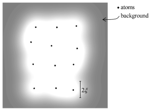
Figure 5: Illustration of the continuous background, modelling the amorphous matrix. Outside the crystallites it has a homogeneous scattering density $\varrho_{0}$, which matches the mean scattering density of the crystallites. In this illustration $\xi$ is $0.45$ times the mean nearest neighbour distance.

This completes the specification of our model and we proceed to compute the scattering function as predicted by the model.

3 Scattering function

Given the atomic positions ${\bf r}_{{\bf m},k}^{(j)}$, the background density $\varrho({\bf r})$ and the statistics of the crystallites’ orientations and positions, we calculate the scattering function:

$$G({\bf q})=$$

$$\Biggl{\langle}\Biggl{|}\sum_{j=1}^{N}\sum_{{\bf m}}^{\bf M}\sum_{k=1}^{K}f_{k}\exp(i{\bf q}{\bf r}_{{\bf m},k}^{(j)})+\int d^{3}r\,\varrho({\bf r})\exp(i{\bf q}{\bf r})\Biggr{|}^{2}\Biggr{\rangle}$$

(8)

Here $\varrho({\bf r})$ is the background intensity whose Fourier transform reads:

$$\int d^{3}r\,\varrho({\bf r})\exp(i{\bf q}{\bf r})$$ (9)

$$= \int d^{3}r\exp(i{\bf q}{\bf r})\left(\varrho_{0}-\bar{f}\sum_{j=1}^{N}\sum_{{\bf m}}^{\bf M}\sum_{k=1}^{K}V({\bf r}-{\bf r}_{{\bf m},k}^{(j)})\right)$$

$$= \varrho_{0}V\delta_{{\bf q},{\bf 0}}-\tilde{V}({\bf q})\sum_{j=1}^{N}\sum_{{\bf m}}^{\bf M}\sum_{k=1}^{K}\exp(i{\bf q}{\bf r}_{{\bf m},k}^{(j)})\,$$

The uniform density, giving rise to a contribution proportional to $\delta_{{\bf q},{\bf 0}}$, does not contain information about the structure of the system. Furthermore the central beam has to be gated out in the analysis of the experimental data. Hence we neglect the uniform contribution and obtain for the scattering intensity (8)

$$G({\bf q})=\left\langle\Bigg{|}\sum_{j=1}^{N}\sum_{{\bf m}}^{\bf M}\sum_{k=1}^{K}\underbrace{\left(f_{k}-\tilde{V}({\bf q})\right)}_{F_{k}({\bf q})}\exp(i{\bf q}\cdot{\bf r}_{{\bf m},k}^{(j)})\Bigg{|}^{2}\right\rangle\,.$$ (10)

The cavities give rise to effective form factors $F_{k}({\bf q})=f_{k}-\tilde{V}({\bf q})$ accounting for the scattering of the atoms themselves, $f_{k}$, and the cavities around them, $\tilde{V}({\bf q})$. Note that, if we want to switch off the background $\bar{f}\to 0$, we return to the original form factors $F_{k}({\bf q})\to f_{k}$.

Inserting the average $\langle\;\;\rangle$ and multiplying out the magnitude squared in (10) yields:

$$G({\bf q})= {\displaystyle\int} \prod_{j=1}^{N}\left(d^{3}{\!R}^{(j)}\mathcal{D}\underline{\underline{D}}^{(j)}\right)\,\mathcal{P}_{\rm pos}({\bf R}^{(1)},...,{\bf R}^{(N)})$$ (11)

$$\times \sum_{j,j^{\prime}=1}^{N}\exp\left(i{\bf q}({\bf R}^{(j)}-{\bf R}^{(j^{\prime})})\right)$$

$$\times \sum_{{\bf m},{\bf m}^{\prime}}^{\bf M}\sum_{k,k^{\prime}=1}^{K}F_{k}({\bf q})F_{k^{\prime}}^{*}({\bf q})$$

$$\times \exp\!\left(i{\bf q}(\underline{\underline{D}}^{(j)}{\bf r}_{{\bf m},k}-\underline{\underline{D}}^{(j^{\prime})}{\bf r}_{{\bf m}^{\prime},k^{\prime}})\right)$$

Note, that the double sum over the crystallites $j$ and $j^{\prime}$ also applies to the rotation matrices $\underline{\underline{D}}^{(j)}$ and $\underline{\underline{D}}^{(j^{\prime})}$ in the second line. We now split the scattering function in two terms $G({\bf q})=G_{1}({\bf q})+G_{2}({\bf q})$: The first one, $G_{1}({\bf q})$, only includes the terms $j=j^{\prime}$ of that sum and thus incorporates scattering of the same crystallite, but not scattering from different crystallites. The second one, $G_{2}({\bf q})$, only including the terms with $j\neq j^{\prime}$, takes into account coherent scattering of two different crystallites.

3.1 Incoherent part

We first consider the case $j=j^{\prime}$ of the sum, i.e. the contribution to the scattering function which is incoherent with respect to different crystallites. Here, the term $\exp(i{\bf q}({\bf R}^{(j)}-{\bf R}^{(j^{\prime})}))$ gives $1$, and therefore the integral over the crystallite positions ${\bf R}^{(j)}$ can be performed and trivially gives 1 due to the normalization of the spatial distribution $\mathcal{P}_{\rm pos}({\bf R}^{(1)},...,{\bf R}^{(N)})$. Furthermore, for each summand $j$, all integrations over the orientations $\underline{\underline{D}}^{(1)},...,\underline{\underline{D}}^{(N)}$, except $\underline{\underline{D}}^{(j)}$, can be performed and also yield 1. Therefore, the $N$ terms with $j=j^{\prime}$ simplify to:

$$G_{1}({\bf q}) = N\int\mathcal{D}\underline{\underline{D}}\,\sum_{{\bf m},{\bf m}^{\prime}}^{\bf M}\sum_{k,k^{\prime}=1}^{K}F_{k}({\bf q})F_{k^{\prime}}^{*}({\bf q})$$ (12)

$$\qquad\qquad\qquad\times\exp\!\left(i{\bf q}(\underline{\underline{D}}{\bf r}_{{\bf m},k}-\underline{\underline{D}}{\bf r}_{{\bf m}^{\prime},k^{\prime}})\right)$$

$$= N\int\mathcal{D}\underline{\underline{D}}\left|\sum_{{\bf m}}^{\bf M}\sum_{p=1}^{P}F_{k}({\bf q})\exp\!\left(i(\underline{\underline{D}}^{T}{\bf q})\cdot{\bf r}_{{\bf m},k}\right)\right|^{2}$$

$$= N\int\mathcal{D}\underline{\underline{D}}\left|A(\underline{\underline{D}}^{T}{\bf q})\right|^{2},$$

where $\underline{\underline{D}}^{T}$ is the transpose of the matrix $\underline{\underline{D}}$ and

$$A({\bf q}):=\sum_{{\bf m}}^{\bf M}\sum_{k=1}^{K}F_{k}({\bf q})\exp(i{\bf q}\cdot{\bf r}_{{\bf m},k})$$ (13)

is the unaveraged scattering amplitude of a single unrotated crystallite. Hence the interpretation of the incoherent part $G_{1}({\bf q})$ is straightforward: Each crystallite contributes independently, each with a given orientation. The orientation can be absorbed in the scattering vector ${\bf q}\to\underline{\underline{D}}^{T}{\bf q}$, so that the contributions of two crystallites with different orientations are simply related by a rotation of the scattering vector. In the macroscopic limit we are allowed to average over all possible orientations and get a sum of $N$ identical terms.

3.2 Coherent part

We now consider the contribution to the scattering intensity from different crystallites, i.e. the case $j\neq j^{\prime}$ in Eq.(11). In analogy to the above calculation all integrations over the orientations $\underline{\underline{D}}^{(1)},...,\underline{\underline{D}}^{(N)}$, can be performed except for $\underline{\underline{D}}^{(j)}$ and $\underline{\underline{D}}^{(j^{\prime})}$:

$$G_{2}({\bf q}) = \int d^{3}\!R^{(1)}\cdots d^{3}\!R^{(N)}\,\mathcal{P}_{\rm pos}({\bf R}^{(1)},...,{\bf R}^{(N)})$$ (14)

$$\times \sum_{j\neq j^{\prime}}\exp\!\left(i{\bf q}({\bf R}^{(j)}-{\bf R}^{(j^{\prime})})\right)$$

$$\times \int\mathcal{D}\underline{\underline{D}}\,\mathcal{D}\underline{\underline{D}}^{\prime}\sum_{{\bf m},{\bf m}^{\prime}}^{\bf M}\sum_{k,k^{\prime}=1}^{K}F_{k}({\bf q})F_{k^{\prime}}^{*}({\bf q})$$

$$\times \exp\!\left(i{\bf q}(\underline{\underline{D}}{\bf r}_{{\bf m},k}-\underline{\underline{D}}^{\prime}{\bf r}_{{\bf m}^{\prime},k^{\prime}})\right)$$

where we have used that the angular distribution is the same for all crystallites. We introduce the structure factor of the crystallite positions:

$$S({\bf q}) = \frac{1}{N}\left\langle\sum_{j,j^{\prime}=1}^{N}\exp\!\left(i{\bf q}({\bf R}^{(j)}-{\bf R}^{(j^{\prime})})\right)\right\rangle$$ (15)

$$= 1+\frac{1}{N}\int d^{3}\!R^{(1)}\cdots d^{3}\!R^{(N)}\,\mathcal{P}_{\rm pos}({\bf R}^{(1)},...,{\bf R}^{(N)})$$

$$\qquad\qquad\times\sum_{j\neq j^{\prime}}\exp\!\left(i{\bf q}({\bf R}^{(j)}-{\bf R}^{(j^{\prime})})\right)\,$$

and observe that the two upper lines in (14) are just $N\left(S({\bf q})-1\right)$. Hence $G_{2}$ can be simplified to:

$$G_{2}({\bf q}) = N\left(S({\bf q})-1\right)$$ (16)

$$\times\left|\int\mathcal{D}\underline{\underline{D}}\,\sum_{{\bf m}}^{\bf M}\sum_{k=1}^{K}F_{k}({\bf q})\exp\!\left(i(\underline{\underline{D}}^{T}{\bf q})\cdot{\bf r}_{{\bf m},k}\right)\right|^{2}$$

$$= N\left(S({\bf q})-1\right)\left|\int\mathcal{D}\underline{\underline{D}}\,A(\underline{\underline{D}}^{T}{\bf q})\right|^{2}$$

Again the interpretation is straightforward: For coherent scattering the amplitudes of individual crystallites with different orientations add up, as expressed by $\int\mathcal{D}\underline{\underline{D}}\,A(\underline{\underline{D}}^{T}{\bf q})$. Spatial correlations of the centers of the crystallites are accounted for by the structure function.

The total scattering function

$$\frac{G({\bf q})}{N}=\int\mathcal{D}\underline{\underline{D}}\left|A(\underline{\underline{D}}^{T}{\bf q})\right|^{2}+\left(S({\bf q})-1\right)\left|\int\mathcal{D}\underline{\underline{D}}\,A(\underline{\underline{D}}^{T}{\bf q})\right|^{2}$$ (17)

is reduced to the scattering amplitude of a single crytallite $A({\bf q})$, which we compute next. Note that if the angular spread of the crystallites can be neglected, in other words all crystallites are approximately aligned, then the above expression reduces to $G({\bf q})=NS({\bf q})\left|A({\bf q})\right|^{2}$, as one would expect.

If there is thermal motion of the atoms around their equilibrium positions due to finite temperature, the intensity of the scattering function $G({\bf q})$ is weakened for larger $q$-values (e.g. willis75, ). The resulting scattering function has to be multiplied with the Debye-Waller factor

$$G_{\text{D}W}({\bf q})=G({\bf q})\cdot\exp(-{\bf q}^{2}\langle u^{2}\rangle)\,,$$ (18)

where $\langle u^{2}\rangle$ is the mean square displacement of the atoms in any direction.

3.3 Scattering amplitude of a single crystallite

The calculation of the scattering amplitude of a single crystallite $A({\bf q})$ (defined in Eq. 13) follows standard procedures. We substitute the atomic positions of Sec. 2.2 and note that the sums over $m_{x}$, $m_{y}$ and $m_{z}$ are geometric progressions which can easily be performed, yielding:

$$A({\bf q})=L_{M_{x}}({\bf q}{\bf a}_{x})L_{M_{y}}({\bf q}{\bf a}_{y})L_{M_{z}}({\bf q}{\bf a}_{z})\sum_{k=1}^{K}F_{k}({\bf q})\exp(i{\bf q}{\bf r}_{k})\,.$$ (19)

Here $L_{M_{\nu}}({\bf q}{\bf a}_{\nu})=\frac{\sin({\bf q}{\bf a}_{\nu}M_{\nu}/2)}{\sin({\bf q}{\bf a}_{\nu}/2)}$ is the well-known Laue function, which has an extreme value, when its argument ${\bf q}{\bf a}_{\nu}$ is a multiple of $2\pi$. It is noteworthy, however, that the position of the extremum of the magnitude of the scattering amplitude $A({\bf q})$ may be shifted, if the form factor of the unit cell $\sum_{k=1}^{K}F_{k}({\bf q})\exp(i{\bf q}{\bf r}_{k})$ has a non-vanishing gradient at that position and $M_{\nu}$ is finite (and therefore the peak width of the Laue function is nonzero). In this case the resultant peak may be shifted by a value of the order of its peak width. Consequently care has to be taken, when determining lattice constants from experimental peak positions.

4 Atomic configuration of the unit cell

The computation of the scattering function $G({\bf q})$ requires the atomic configuration $\{{\bf r}_{k}\}_{k=1}^{K}$ of the unit cell, which we discuss next.

4.1 Unshifted unit cells

It is known that the crystallites are composed of poly-alanine strands (see arnott67 ; grubb97 ). In Fig. 6, two alanine amino acids of this strand are shown. Its conformation, shown on the right side, is well established and was created with Yasara meling2006 . There are two constraints for the strand: First, the subsequent alanines in the strand must have the same orientation so that the strand does not have a “twist” and can produce periodic structures. Second, the distance between adjacent alanines has to match the size of the unit cell. These two constraints allow for a unique choice of the two degrees of freedom, namely the Ramachandran angles ramachandran $\Phi$ and $\Psi$ which are the dihedral angles for the bonds C_α-N and C_α-C, respectively.

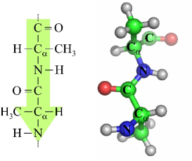
Figure 6: (Color online) Chemical structure (left) and conformation (right) of a poly-alanine strand. Two alanines are shown. The CH₃ group is characteristic for the alanine amino acid and is bound to the so called C_α atom. The arrow indicates the direction ${\rm C}\rightarrow{\rm C}_{\alpha}\rightarrow{\rm N}$ of the backbone.

Many of the described poly-alanine strands side by side form a stable crystalline configuration, the $\beta$-pleated-sheet. We assume an orthorombic unit cell , consisting of four alanine strands, as illustrated in Fig. 7. Thus one unit cell contains 8 alanine amino acids. Furthermore we define the spatial directions in the usual way (e.g. warwicker, ):

• Direction of the CH₃-groups and Van-der-Waals interactions between sheets lying upon each other.

• Direction of the hydrogen bonds between the O-atom of one strand and the H-atom of the neighboring strand.

• Direction of the covalent bonds along the backbone.

Accordingly, ${\bf a}_{x}$, ${\bf a}_{y}$ and ${\bf a}_{z}$ are the principal vectors pointing in these directions and $a_{x}$, $a_{y}$, $a_{z}$ their magnitudes. Note furthermore that due to symmetry the distance between the strands has to be $a_{x}/2$ in the $x$-direction and $a_{y}/2$ in the $y$-direction.

In general one has to distinguish between the parallel and antiparallel structure. In the parallel structure the direction of the atom sequence ${\rm C}\rightarrow{\rm C}_{\alpha}\rightarrow{\rm N}$ in the strand’s backbone is the same for all strands (left side of Fig. 7). For the antiparallel structure, this direction is alternating along the $y$-axis (right side of fig. 7). Both will be considered in the following analysis.

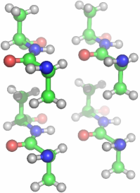
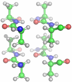
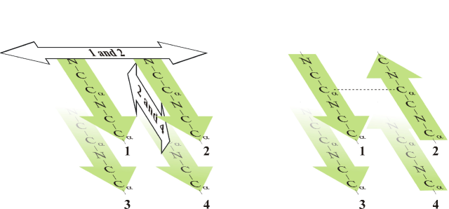
Figure 7: (Color online) Illustration of one unit cell, containing four neighboring poly-alanine strands. Top: configuration of the atoms. Center: Schematic view displaying only the backbone atoms. The arrows illustrate two possible adjustments of the structure, which are to be optimzied to match the experimental scattering image. Bottom: Simplified schematic view along the backbone axis ${\bf a}_{z}$, where $\odot$ indicates an arrow pointing towards the reader and $\otimes$ pointing away from the reader. Here the unit cell is shown as a gray rectangle. In each case, a parallel structure is shown on the left side, and an antiparallel structure on the right side. The illustration shows an unshifted configuration, that means: The C_α atoms of neighboring strands are aligned and have no shift in $z$-direction (indicated as dashed line in the middle right image). Furthermore, the strands are exactly aligned in the $x$- and $y$-direction.

4.2 Possible shifts inside the unit cell

The scattering intensity is not only sensitive to the conformation of the poly-alanine strands, but also to the distance and orientation of different strands relative to each other. Besides the question of parallel or antiparallel structure, the four strands can also be shifted with respect to each other. In principle there are four ways to displace them (see Fig. 7):

• Shifting strands 1 and 2 in the $y$-direction by a value $\Delta y_{12}$. This displacement is performed in Fig. 8.

• Shifting strands 1 and 2 in the $z$-direction by a value $\Delta z_{12}$. Because of the CH₃-groups extending into the layers above and below (as seen in Fig. 7, top panel), a displacement like this is only possible, if those two strands have a shift in the $y$-direction of $\Delta y_{12}\approx\pm{\bf a}_{y}/4$, as well. In this case the CH₃-groups can pass each other without overlapping.

• Shifting strands 2 and 4 in the $z$-direction by a value $\Delta z_{24}$. This shift was originally suggested by Arnott et al. arnott67 .

• Shifting strands 2 and 4 in the $x$-direction. However this displacement would have a high energy cost, because it would break the hydrogen bonds between the H- and O-atoms of neighboring strands. Since, moreover, no reasonable result could be achieved performing such shifts, it will not be included in our discussion any further.

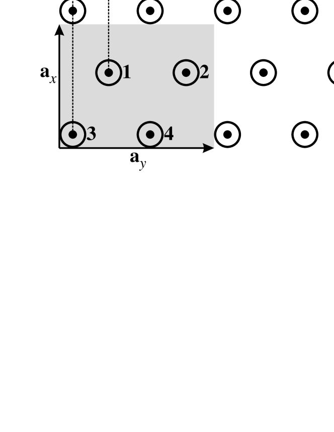
Figure 8: Illustration of the unit cell, as at the bottom of Fig. 7, but with the conducted shift $\Delta y_{12}=a_{y}/4$ of strands 1 and 2 the in $y$-direction.

Note that shifting strands 1 and 2 in the $x$-direction or strands 2 and 4 in the $y$-direction is associated with resizing the unit cell in the $x$- or $y$-direction, respectively.

4.3 Variations between crystallites

For real systems, the composition of the crystallite is certainly not fixed, but may vary from crystallite to cyrstallite. These variations can easily be included into our model introducing a probability distribution $P(\{r_{{\bf m},k}\})$ for the crystallite configuration $\{r_{{\bf m},k}\}$, with the normalization $\sum_{\{r_{{\bf m},k}\}}P(\{r_{{\bf m},k}\})=1$. The calculation is performed completely analogous to orientational distribution. The scattering function becomes

$$\frac{G({\bf q})}{N} = \sum_{\{r_{{\bf m},k}\}}P(\{r_{{\bf m},k}\})\int\mathcal{D}\underline{\underline{D}}\left|A(\underline{\underline{D}}^{T}{\bf q})\right|^{2}$$

$$+ \left(S({\bf q})-1\right)\left|\sum_{\{r_{{\bf m},k}\}}P(\{r_{{\bf m},k}\})\int\mathcal{D}\underline{\underline{D}}\,A(\underline{\underline{D}}^{T}{\bf q})\right|^{2}\,.$$

Later (sec. 5.2) we will investigate the effect of variable crystallite sizes as well as the influence of small fractions of glycine inside the crystallites.

5 Results

5.1 Experimental scattering function

Two types of samples have been investigated: fiber bundles and single fiber preparations. Single fibers demand a highly collimated and brilliant beam, but are better defined in orientation and are amenable tosimultaneous strain-stress measurements.

An oriented bundle of major ampullate silk (MAS) of Nephilia Clavipes was measured at the D4 bending magnet of HASYLAB/DESY in Hamburg. The fibers were reeled on a steel holder and oriented horizontally in the beam. The estimated number of threads was 400-600. Photon energy was set to $E=10.9$ keV by a Ge(111) crystal monochromator located behind a mirror to suppress higher harmonics. Data was collected with a CCD x-ray camera (SMART Apax, AXS Bruker) with 60$\,\mu$m pixel size and an active area of $62\,{\rm cm}\times 62\,{\rm cm}$. Illumination was triggered by a fast shutter. The momentum transfer was calibrated by a standard (corrundum). Raw data was corrected by empty image (background subtracted).

The single fiber experiments have been carried out at the microfocus beamline ID13 at ESRF, Grenoble id13 . A 12.7 keV x-ray beam was focused with a pair of short focal length Kirkpatrick Baez (KB) mirrors KB to a $7\mu m$ spot at the sample. This focusing scheme provides a sufficient flux density ($6.8\cdot 10^{15}cps/mm^{2}$) to obtain diffraction patterns from single dragline fibers. The single fiber diffraction patterns were recorded with a CCD detector positioned 131 mm behind the sample (Mar 165 detector, Mar USA, Evanston, IL). One of the beamline’s custom made lead beamstops (approx. 300$\mu m$ diameter) was used to block the intense primary beam. The raw data was treated as follows: (i) both the image and the background (empty beam) were corrected by dark dark current, and (ii) the (empty beam) background was subtracted from the image. The peaks which are significantly broadened by the small crystallite size (see below) can then be indexed to the orthorombic lattice described above. Typical scattering distribution for both types of sample preparations are shown in fig. 9 as a function of parallel and vertical momentum transfer. More details on experimental procedures and on the sample preparation by forced silking can be found in GlisovicAPA07 ; Glisovic08 .

5.2 Scattering function from the model

It is our aim to determine those crystallites’ parameters, which best match the experimental result. The free parameters of our model are the three shifts $\Delta y_{12}$, $\Delta z_{12}$ and $\Delta z_{24}$, the unit cell dimensions $a_{x}$, $a_{y}$ and $a_{z}$, the crystallite size in the three directions $M_{x}$, $M_{y}$ and $M_{z}$, as well as $\theta_{0}$, the tilting angle of the crystallites away from the fiber axis.

The parameters of our model affect the scattering intensity in different ways, which allows us to at least partially separate the effects of different parameters. The crystallite size $(M_{x},M_{y},M_{z})$ determines the peak widths, whereas the length of the principal vectors ${\bf a}_{x}$, ${\bf a}_{y}$ and ${\bf a}_{z}$ determine the peak position. (We have to keep in mind, however, that the peak position can differ from the extremal values of the Laue functions, as explained in section 3.3.) The shifts $\Delta y_{12}$, $\Delta z_{12}$ and $\Delta z_{24}$, as described in Sec. (4.2), affect the relative peak intensities via the form factors of the unit cell, $\sum_{k=1}^{K}F_{k}({\bf q})\exp(i{\bf q}{\bf r}_{k})$. Finally, the parameter $\theta_{0}$ is responsible for the peak widths in the azimuthal direction on the scattering image.

	presented calculation		Warwicker warwicker54	Marsh marshShort	Arnott arnott67
structure of	Nephila clavipes		Bombyx mori	Tussah Silk	poly-L-alanine
alignement	parallel	anti-parallel	anti-parallel	anti-parallel	anti-parallel
$a_{x}$	$10.0\;\text{\AA}$	$10.0\;\text{\AA}$	$10.6\;\text{\AA}$	$10.6\;\text{\AA}$	$10.535\;\text{\AA}$
$a_{y}$	$9.3\;\text{\AA}$	$9.3\;\text{\AA}$	$9.44\;\text{\AA}$	$9.44\;\text{\AA}$	$9.468\;\text{\AA}$
$a_{z}$	$6.95\;\text{\AA}$	$6.95\;\text{\AA}$	$6.95\;\text{\AA}$	$6.95\;\text{\AA}$	$6.89\;\text{\AA}$
$M_{x}$	1.5 (∗)	1.5 (∗)	-	-	-
$M_{y}$	5	5	-	-	-
$M_{z}$	9	9	-	-	-
$\Delta y_{12}$	$a_{y}/4$	$a_{y}/4$	0	$a_{y}/4$	$\pm a_{y}/4$ (∗∗)
$\Delta z_{12}$	$0$	$0$	0	0	0
$\Delta z_{24}$	$0$	$-a_{z}/6$	0	0	$-a_{z}/10$
$\theta_{0}$	$7.5^{\circ}$	$7.5^{\circ}$	-	-	-
$\langle u^{2}\rangle$	0.1 Å2	0.1 Å2	-	-	-

Table 1: Summary of parameters. The left two columns show the best match between experimental and calculated scattering functions. For $a_{z}=6.95\;\text{\AA}$, the resulting Ramachandran angles are $\Phi=-139.0^{\circ}$ and $\Psi=136.9^{\circ}$. $\langle u^{2}\rangle$ was used for the Debye-Waller factor in eq. (18). The three right columns compare our obtained parameters with the literature.
^(∗) Note that each unit cell contains two layers of alanin-strands in $x$-direction. Therefore $M_{x}=1.5$ corresponds to three layers of $\beta$-sheets in a single crystallite.
^(∗∗) Statistical model: A layer is shifted by a value $+a_{y}/4$ or $-a_{y}/4$ with respect to the previous layer, where $+$ and $-$ are equally likely.

From Eq. (19) it is clear that the $z$-components of the atom positions $\{{\bf r}_{k}\}_{k=1}^{K}$ are irrelevant for the scattering amplitude $A({\bf q})$ in the $xy$-plane, i.e. if the $z$-component of ${\bf q}$ is zero. Therefore, parameters affecting only the $z$-components – especially the mentioned shifts in the $z$-direction – will not influence the intensity profile of $G({\bf q})$ in the $xy$-plane. Analogously, the scattering profile in the $z$-direction is independent of parameters influencing the $x$- and $y$-directions. Consequently, the sections of the scattering profile along and perpendicular to the fiber axis can be matched to subsets of the parameters separately. The intensity profile off the $z$- and $xy$-axes, taking into account all dimensions of the crystallite, can be seen as a consistency check for the found parameters.

The experimental scattering data clearly reveal a (002) peak, Fig. 9. This peak is allowed by symmetry, however it is extremely weak in the antiparallel structure suggested by Marsh marshShort and shown in Fig. 10. The reason is the following: the electron density within the unit cell projected along the $z$-axis is almost uniform, varying by approximately $10\%$. We therefore propose two alternative mechanisms generalizing the classical (Marsh) model of the antiparallel unit cell. By both mechanisms the intensity of the (002) peak will increase in agreement with the experiment:

• the shift of strands 2 and 4 in the $z$-direction, i.e. a nonzero $\Delta z_{24}$-shift or

• structural disorder affecting the almost uniform electron density.

We first discuss case a). The uniform electron density is disturbed by a shift $\Delta z_{24}\neq 0$. The intensity of the (002)-reflection grows accordingly with an increasing shift $\Delta z_{24}$. Adjusting the $\Delta z_{24}$-shift yields results consistent with experiment.

In table 1 we present the results for the parameters of the model, obtained from optimising the agreement between the calculated scattering function and the experimental one. For comparison we show the set of parameters for both, the parallel and the antiparallel structure. On the basis of the experimental data, one can not discriminate between the parallel and the antiparallel structure.

The scattering intensities, as calculated with these values, are shown in Fig. 11. The crystallites are randomly tilted with respect to the fiber axis, so that on average the system is invariant under rotations around the fiber axis. Consequently the scattering image also has rotational symmetry about the $z$-axis and the $q_{x}$- and $q_{y}$-axis are indistinguishable and denoted by $q_{xy}$. A section along the $q_{xy}$-axis is shown in fig. 12, top panel. The mismatch for $q$-values slightly larger than the (120)-peak is plausible, because in this region the amorphous matrix contributes noticeably to the experimental scattering intensity, but has been neglected in the model. The oscillations of the calculated scattering image for low $q$-values are side maxima which are suppressed by fluctuations in the crystallite sizes (see sec. 4.3). The corresponding scattering intensities are shown in Fig. 12 and Fig. 14, left. Clearly the side maxima have been suppressed.

We now discuss an alternative mechanism to generate a stronger (002) peak, e.g. by introduction of disorder in the amino acid composition of the unit cell (case b). Poly-alanine as a model for the crystallites in spider silk is an over-simplification, since the amino acid sequence hardly allows for a pure poly-alanine crystallite. Instead we expect that other residues must be incorporated into the crystallite even if energetically less favorable to compromise the given sequence. In particular, it is highly likely that also glycine amino acids are embedded in the crystallites marsh . This can be easily implemented by replacing randomly selected alanine amino acids of the crystallites with glycine (see sec. 4.3). It is found that the intensity of the (002) peak increases with the fraction of susbstituted alanines. In Fig. 10 we compare the original Marsh-structure (without gylcine) to a structure with the same parameters, but with alanine replaced with glycine randomly with a probability $p_{\text{gl}}=0.375$. The random substitution has clearly produced an intensity of the (002) peak comparable to experiment.

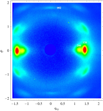
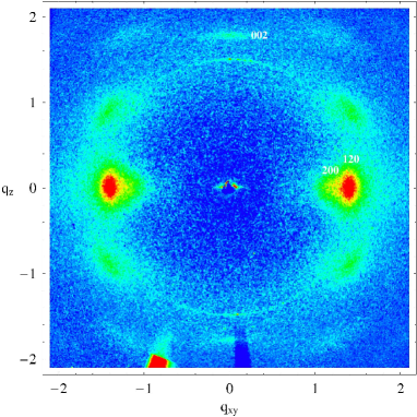
Figure 9: (Color online) Scattering images of spider silk. The fiber axis runs vertical. On top, the colorbar shows scattering intensities, which are normalized by the intensity of the (120)-peak. Below the experimental scattering image of spider silk from Nephila clavipes is shown, both for bundle measurements (left) and single fiber diffraction (right)

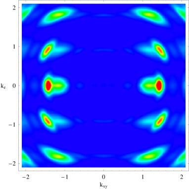
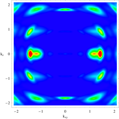
Figure 10: (Color online) Calculated scattering images of the structure proposed by Marsh et al. marshShort . Unit cell size: $(a_{x},a_{y},a_{z})=(10.6,9.44,6.95)$ and we used the crystallite size $(M_{x},M_{y},M_{z})=(1.5,6,9)$. Left: The crystallites are purely made of alanine amino acids. Right: The crystallites’ alanine amino acids are replaced with glycine with a probability $p_{\text{gl}}=0.375$.

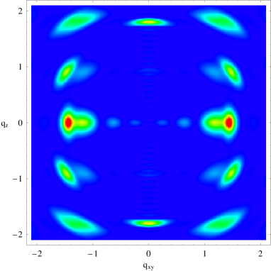
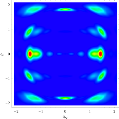
Figure 11: (Color online) Scattering images, as calculated from eq. (17), for the parallel structure on the left side and the antiparallel structure on the right side.

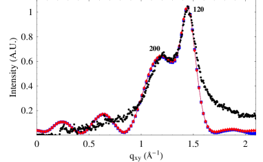
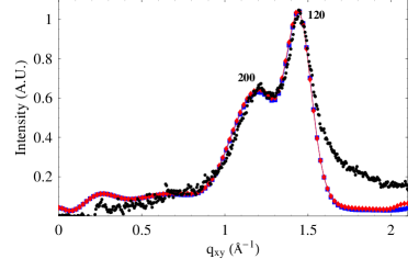
Figure 12: (Color online) Top: Comparison of a section of the experimental ($\bullet$) and the calculated scattering intensity ( ${\color[rgb]{0,0,1}{\scriptstyle\blacksquare}\!\!\!\!\!\!\frac{\;\;\;\;\,}{\,}}$ parallel,  ${\color[rgb]{1,0,0}{\blacklozenge}\!\!\!\!\!\!\frac{\quad}{\,}}$ antiparallel). Sections of the profiles in Fig. 11 along the $q_{xy}$-axis, i.e. the scattering profile perpendicular to the fiber axis, are shown. Bottom: as top, but with a Gaussian distribution (rounded to integers) of the crystallite sizes $M_{x}$, $M_{y}$ and $M_{z}$. The widths are $\Delta M_{x}=2$, $\Delta M_{y}=0.75$ and $\Delta M_{z}=3$ respectively.

6 Conclusions

We have developed a microscopic model of the structure of spider silk. The main ingredients of the model are the following:

• Many small crystallites are distributed randomly in an amorphous matrix,

• the orientation of the crystallites fluctuate with a preferential alignment along the fiber axis,

• each crystallite is composed typically of $5\times 2\times 9$ unit cells,

• each unit cell contains four alanine strands, constructed with Yasara and shifted with respect to each other. Disorder can be generated by randomly replacing alanine with glycine.

We have computed the scattering intensity of our model and compared it to wide-angle x-ray scattering data of spider silk. Possible inter-crystallite correlations are unimportant, given the measured orientational distribution. In other words, even if significant center-of-mass correlations between crystallites were present, the orientational distribution would suppress interference effects, with the exception of the (002) peak, which is least sensitive to orientational disorder. The contribution of coherent scattering is discussed in detail in Appendix B.

A homogeneous electron density background is a necessary feature of the scattering model. Calculation of the crystal structure factor in vacuum does not only lead to an incorrect overall scaling prefactor (which is important if absolute scattering intensities are measured), but also leads to a scattering intensity distribution with artifacts at small and intermediate momentum transfer.

The comparison between model and data fixes the parameters of the unit cell and the crystallite for the two possible cases, the parallel and the antiparallel structure, respectively, as shown in Table 1. The two models with parallel and antiparallel alignment of the alanine strands yield comparable agreement with the experimental data. Also a refined model in which alanine is randomly replaced with glycine give reasonable results. Hence we cannot rule out one of these structures.

Our model is similar to the model of the poly-L-alanine of Arnott et al. arnott67 . Their model does incorporate a $\Delta z_{24}$-shift. However, our structure shows a better agreement with the experimentally measured scattering function using a value of $\Delta z_{24}=-a_{z}/6$.

While we have concentrated here on the wide-angle scattering reflecting the crystalline structure on the molecular scale, we note that the same model can be used for small-angle scattering to analyze the short range order between crystallites in the presence of orientational and positional fluctuations. In particular, the model can describe the entire range of momentum transfer and the transition from wide angle scattering (WAXS) to small angle scattering (SAXS). Note that WAXS is usually described only in the single object approximation, neglecting inter-particle correlations. Contrarily, SAXS is mostly described in contiunuum models without crystalline parameters. Here both are treated by the same approach, which is a significant advantage for systems where the length scales are not decoupled.

Acknowledgments

We thank Martin Meling for a beneficial discussions and cooperation on the construction of the parallel and antiparallel raw structures of the $\beta$-sheets. We gratefully acknowledge financial support by the Deutsche Forschungsgemeinschaft (DFG) through Grant SFB 602/B6.

Appendix

Appendix A Effect of the continuous background

In this section we explain why it is necessary to include the continuous background between the crystallites, introduced in section 2.4.

Without the background, the system has vast, unphysical density fluctuations on the length scale of the crystallite distances, resulting in a large scattering function $G({\bf q})$ for small $q$-values. As already explained in section 2.4, these density fluctuations are unphysical, because the space between the crystallites is filled with the amorphous matrix and water molecules. Fig. 13 shows the the scattering profiles in $xy$-direction with and without the continuous background. As expected the system without the background shows a large increase of the scattering function for small $q$-values. The countinous background, howerver, acts as a low-pass filter on the scattering density and therefore annihilates the large intensities for small $q$.

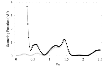
Figure 13: Scattering function in $xy$-direction with ($\scriptstyle\square$) and without ($\scriptstyle\blacksquare$) continuous background. Without background, density fluctuations on large length scales cause an increase of the scattering function for small $q$-values.

Appendix B Relevance of the coherent part of the scattering function

Here we discuss the infulence of the coherent part of the scattering function of eq. (17). Fig. 14 shows a comparison of the incoherent part

$$G_{1}({\bf q})=\int\mathcal{D}\underline{\underline{D}}\left|A(\underline{\underline{D}}^{T}{\bf q})\right|^{2}\,,$$ (21)

which is used to calculated the scattering function in this paper, and the contribution

$$G^{\prime}_{2}({\bf q}):=\left|\int\mathcal{D}\underline{\underline{D}}\,A(\underline{\underline{D}}^{T}{\bf q})\right|^{2}$$ (22)

of the coherent part $G_{2}({\bf q})=\left(S({\bf q})-1\right)\left|\int\mathcal{D}\underline{\underline{D}}\,A(\underline{\underline{D}}^{T}{\bf q})\right|^{2}$.

Neglecting the coherent part is plausible for two reasons. Firstly, because the contribution of $G^{\prime}_{2}({\bf q})$ is small compared to the incoherent part $G_{1}({\bf q})$, as seen in the figure. And secondly, the length scale for the distances between the crystallites is much larger than atom length scales investigated here. On length scales we are interested in, we expect $S({\bf q})\approx 1$, assuming that the crystallite positions have no long range order. Therefore, the prefactor $\left(S({\bf q})-1\right)$ additionally reduces contribution of the coherent term.

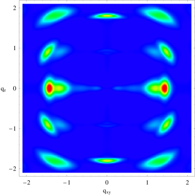
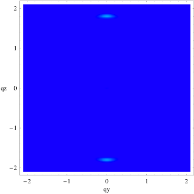
Figure 14: (Color online) Left: Calculated scattering images as in Fig. 11, but for a Gaussian distribution (rounded to integers) of the crystallite sizes $M_{x}$, $M_{y}$ and $M_{z}$. The widths are $\Delta M_{x}=2$, $\Delta M_{y}=0.75$ and $\Delta M_{z}=3$ respectively. Right: correlated part $G^{\prime}_{2}({\bf q})$ of the scattering function eq. (17) in comparison to the uncorrelated part (left).

The (002)-peak is special for the coherent scattering term $G^{\prime}_{2}({\bf q})$. All peaks except for the (002)-peak have a very small contribution in $G^{\prime}_{2}({\bf q})$ because of the white average of the crystallites’ rotations about the fiber axis, which makes coherent scattering from different crystallites less likely, no matter how the crystallites are arranged in space. Since there is a preferential alignment of the crystallites in $z$-direction, however, contributions of coherent scattering from different crystallites (which are contained in the term $G^{\prime}_{2}({\bf q})$) are not completely destroyed; therefore, if the crystallites’ distance in $z$ direction is a multiple of the unit cell size $a_{z}$, causing a large contribution in the prefactor $\left(S({\bf q})-1\right)$ at the position of the (002)-peaks, a contribution of $G_{2}({\bf q})$ would be present.

References

- (1) D. Grubb, L. Jelinski, Macromolecules 30, 2860 (1997)
- (2) S. Fossey, D. Kaplan, Polymer Data Handbook (Oxford University Press, 1999), chap. Silk Protein
- (3) J. Gosline, P. Guerette, C. Ortlepp, K. Savage, The Journal of Experimental Biology 202, 3295 (1999)
- (4) D. Kaplan, W. Adams, B. Farmer, C. Viney, eds., Silk Polymers - Material Science and Biotechnology, ACS Symposium Series 554 (American Chemical Society, Washington, DC, 1994)
- (5) D. Huemmerich, T. Scheibel, F. Vollrath, S. Cohen, U. Gat, S. Ittah, Current Biology 14, 2070 (2004)
- (6) T. Scheibel, Microbial Cell Factories 3, 14 (2004)
- (7) D. Huemmerich, U. Slotta, T. Scheibel, Applied Physics A 82, 219 (2006)
- (8) A.W.P. Foo, E. Bini, J. Huang, S. Lee, D. Kaplan, Applied Physics A 82, 193 (2006)
- (9) S. Rammensee, D. Huemmerich, K. Hermanson, T. Scheibel, A. Bausch, Applied Physics A 82, 261 (2006)
- (10) F. Vollrath, D. Porter, Applied Physics A 82, 205 (2006)
- (11) J. Zbilut, T. Scheibel, D. Huemmerich, C. Webber, M. Colafranceschi, A. Guiliani, Applied Physics A 82, 243 (2006)
- (12) R. Puxkandl, I. Zizak, O. Paris, J. Keckes, W. Tesch, S. Bernstorff, P. Purslow, P. Fratzl, Philosophical Transactions of the Royal Society of London, Series B 357, 191 (2002)
- (13) P. Roschger, B. Grabner, S. Rinnerthaler, W. Tesch, M. Kneissel, A. Berzlanovich, K. Klaushofer, P. Fratzl, Journal of Structural Biology 136, 126 (2001)
- (14) J.O. Warwicker, J. Mol. Biol. 2, 350 (1960)
- (15) D. Kaplan, W. Adams, B. Farmer, C. Viney, eds., Silk Polymers, ACS Symposium 544 (American Chemical Society, Washington, DC, 1994)
- (16) D. Grubb, L. Jelinski, Macromolecules 30, 2860 (1997)
- (17) J. van Beek, S. Hess, F. Vollrath, B. Meier, Proceedings of the National Academy of Sciences of the United States of America (PNAS) 99, 10266 (2002)
- (18) C. Riekel, M. Mueller, F. Vollrath, Macromolecules 32, 4464 (1999)
- (19) C. Riekel, B. Madsen, B. Knight, F. Vollrath, Biomacromolecules 1, 622 (2000)
- (20) C. Riekel, F. Vollrath, International Journal of Biological Macromolecules 29, 203 (2001)
- (21) C. Riekel, C. Bränden, C. Craigc, C. Ferreroa, F. Heidelbacha, M. Müller, International Journal of Biological Macromolecules 24, 187 (1999)
- (22) C. Riekel, M. Rössle, D. Sapede, F. Vollrath, Naturwissenschaften 91, 30 (2004)
- (23) D. Sapede, T. Seydel, V. Forsyth, M. Koza, R. Schweins, F. Vollrath, C. Riekel, Macromolecules 38, 8447 (2005)
- (24) A. Glišović, T. Vehoff, R.J. Davies, T. Salditt, Macromolecules 41, 390 (2008)
- (25) R. Marsh, R. Corey, L. Pauling, Biochimica et Biophysica Acta 16, 1 (1955)
- (26) G. Zubay, Biochemistry, 4th edn. (McGraw-Hill Education, 1998)
- (27) B.T.M. Willis, A.W. Pryor, Thermal Vibrations in Crystallography (Cambridge University Press, 1975), chap. 4, 1st edn.
- (28) S. Arnott, S.D. Dover, A. Elliot, J. Mol. Biol. 30, 201 (1967)
- (29) M. Meling, Modellierung und Strukturanalyse von -Faltblattkristalliten in Spinnenseide, Diploma Thesis, Göttingen University (2006)
- (30) C. Ramakrishnan, G.N. Ramachandran, Biophys J. 5, 909 (1965)
- (31) C. Riekel, R.J. Davies, Current Opinion in Colloid & Interface Science 9, 396 (2005)
- (32) P. Kirkpatrick, A.V. Baez, J. Opt. Soc. Am. 38, 766 (1948)
- (33) A. Glišović, T. Salditt, Applied Physics A 87, 63 (2007)
- (34) J.O. Warwicker, Acta Cryst. 7, 565 (1954)
- (35) R. Marsh, R. Corey, L. Pauling, Acta Cryst. 8, 710 (1955)