Anisotropic profiles in the spin polarization of multichannel semiconductor rings with Rashba spin orbit coupling

Abstract

We investigate the spin accumulation effect in eccentric semiconductor multichannel rings with Rashba spin-orbit interaction and threaded by a magnetic flux. Due to the finite eccentricity, the spin polarization induced at the borders of the sample is anisotropic and exhibits different patterns and intensities at specific angular directions. This effect, reminiscent of the spin polarization drift induced by the application of an in plane electric field, could be used to manipulate and functionalize the spin polarization in electronic nanorings.

I Introduction

The spin manipulation and detection in all electrical devices have been the subjects of an impressive amount of research in the last years Awschalom et al. (2002). In particular semiconductors in which the spin orbit (SO) interaction plays a significant role, are the main candidates to accomplish such challenges. Among them, ring shaped geometries are particularly attractive to analize different interference phenomena in the presence of SO effects. As an example, Aharonov Bohm (AB) rings with uniform SO interaction have been proposed as spin interference devices nitta, meijer and takayanagi (1999) to explore the non trivial spin dependent Aharonov-Casher (AC) phase aharonov and casher (1984); Berry (1984); Aronov and Lyanda? Geller (1993). Indeed, in recent years the AC effect has been measured in a series of transport experiments on AB conductance oscillations performed in semiconductor rings, for different intensities of the SO interaction Morpurgo et al (1998); Meijer et al. (2004); koning et al (2006); Bergsten et al (2006).

So far most of the theoretical analysis of SO effects in quantum rings have been restricted to 1D geometries meir gefen and entil-wohlman (1989); loss and goldbart (1992); Balatsky and Althsuler (1993); Chaplik and Magarill (1995); Splettstoesser, Governale and Zülicke (2002); lobos and Aligia (2008). However realistic rings have a multichannel nature and many interesting phenomena rely on this fact. As an example, in Ref.Lozano, Sanchez, 2005 it was shown that in a AB multichannel ring with Rashba SO coupling Bychkov and Rashba (1984), a spin accumulation effect develops at the borders of the sample. Eventhough for an even number of electrons, a finite spin polarization in the direction perpendicular to the plane of the ring is generated and can be controlled with the magnetic flux. This phenomena, although sharing some analogies with the intrinsic Spin Hall Effect (SHE) studied in bar or strip geometries designed on 2DEG Kato et  al. (2004); Sinova et al. (2004); Wunderlich et al. (2005), does not require neither external currents nor electric fields or voltage drops applied usaj and balseiro (2005); reynoso2 .

Actually in real semiconductor quantum rings (QRs) imperfections of the structure often occurs. Micrograph views of GaAs QRs suggests that real rings may present some degree of eccentricity Bang Yau et al. (2002). In addition, recent advances in oxidation lithography enables the fabrication of semiconductor QRs grbic et al. (2007) in which non perfect symmetric structures can be constructed.

The effect of a finite eccentricity has been considered in previous studies of energy spectrum and electric polarization in QRs egydio, mijolaro (2004); bruno, latge (2005). However these works have not taken into account the SO interaction, which is particularly strong in most of the QRs heterostructures.

The goal of the present work is to show that by a combined effect of the Rashba SO interaction and the finite eccentricity, the spin accumulation develops anisotropic patterns along the sample. This effect, that shall be described in detail later on, will lead to different intensities of the total spin polarization in the angular direction. The typical spatial separation of the anisotropic patterns may render possible to sense the effect employing usual magneto optical detection techniques Crooker et al (2005).

The article is organized as follows. Sec.II introduces the model hamiltonian for the eccentric QR with Rashba SO interaction. After giving some details of the calculations, the energy spectrum and eigenfunctions are obtained for different magnetic fluxes. These results are analyzed and compared to the ones of the concentric QR. In Sec.III the spin polarization is computed and the different anisotropic patterns in the spin accumulation effect are analyzed in detailed. The last section IV is devoted to the conclusions and to elaborate on the experimental feasibility to detect the anisotropic profiles in the spin accumulation effect.

II Eigenfunctions and eigenvalues of the eccentric QR with Rashba SO interaction

We start by considering a 2D electron gas in the $xy$ plane confined to an annular region delimited by two circles of radii $a$ and $b$ whose centers $O$ and $O^{{}^{\prime}}$ are separated by a distance $d<b-a$, that defines the eccentricity of the QR. A magnetic flux $\Phi$ threads the structure (see Fig.1).

The single particle Hamiltonian describing an electron of effective mass $m^{*}$ subjected to the Rashba spin orbit (RSO) coupling reads

$$H=\frac{{\bf p}^{2}}{2m^{*}}+V+\frac{\alpha}{\hbar}({\bf p}\times{\bf\hat{\sigma}})\cdot\hat{z}\;,$$ (1)

where $\alpha$ is the strength of the Rashba spin orbit (RSO) coupling and the Pauli matrices ${\bf\hat{\sigma}}$ are defined as standard. Let the polar coordinates be $(\rho,\theta)$ and $(\rho^{\prime},\theta^{\prime})$ with respect to $O$ and $O^{\prime}$ respectively. The confining potential defining the eccentric QR is

$$V(\rho,\theta)=\left\{\begin{array}[]{l}0\;\;\mbox{for $a<\rho<\rho_{ext}\equiv\sqrt{b^{2}+d^{2}-2\;b\;d\;\cos\theta\sqrt{1-(\frac{d}{b}\sin\theta)^{2}}}$ }\\ \infty\;\;\mbox{otherwise}\;.\end{array}\right.$$ (2)

The vector potential which is introduced in the Hamiltonian via the substitution, ${\bf p}=\hbar{\bf k}=-i\hbar{\bf\nabla}-\frac{e}{c}{\bf A}$, is written in the axial gauge as ${\bf A}=(\Phi/2\pi\rho)\hat{\theta}$ . Using , $\hat{\sigma}_{\rho}=\cos\theta\hat{\sigma}_{x}+\sin\theta\hat{\sigma}_{y}$ and $\hat{\sigma}_{\theta}=-\sin\theta\hat{\sigma}_{x}+\cos\theta\hat{\sigma}_{y}$ we can rewrite the Hamiltonian as

$$H=-\frac{\hbar^{2}}{2m^{*}}\left[\frac{1}{\rho}\partial_{\rho}\left(\rho\partial_{\rho}\right)-\frac{1}{\rho^{2}}(i\partial_{\theta}+\nu)^{2}\right]$$

$$+i\alpha\hat{\sigma}_{\theta}\partial_{\rho}-\frac{\alpha}{\rho}\hat{\sigma}_{\rho}\Bigl{(}i\partial_{\theta}+\nu\Bigr{)}\,\,,$$ (3)

where $\nu=\frac{\Phi}{\Phi_{0}}$ is the magnetic flux in units of the flux quantum $\Phi_{0}={hc}{/e}$.

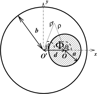
Figure 1: Schematic of the annular cavity with RSO threaded by a finite flux $\Phi$, where $a$ and $b$ are the internal and external radii respectively, and $d$ the eccentricity. $\rho(\rho^{\prime}),\theta(\theta^{{}^{\prime}})$ are the polar coordinates referred to the origin $O(O^{{}^{\prime}})$.

In what follows it will be useful to define the dimensionless coordinates $\xi=\rho/b$, $\xi^{\prime}=\rho^{\prime}/b$, the aspect ratio $\lambda=b/a$ and

$$\epsilon=\frac{2m^{*}b^{2}}{\hbar^{2}}E\equiv\frac{E}{E_{0}}\,\,,\,\,\beta=2\frac{m^{*}\alpha}{\hbar^{2}}b\;.$$ (4)

Due to the RSO, the bulk spectrum has two branches Bychkov and Rashba (1984)

$$\epsilon={(bk)}^{2}\pm\beta\;{(bk)}\;,$$ (5)

and for a given value of $\epsilon$ there are two non-trivial solutions for the momentum $k$ that we denote $k^{+}$ and $k^{-}$ respectively.

For the concentric ring ($d=0$), the total angular momentum $J_{z}=l_{z}+\frac{1}{2}\hbar\hat{\sigma}_{z}$ is a constant of motion and $j=m+\frac{1}{2}$ is a good quantum number even for finite RSO coupling. In Ref.Lozano, Sanchez, 2005 the complete set of eigenfunctions (eigenspinors labeled by the quantum number $j=m+1/2$) and eigenvalues have been found for the concentric QR with RSO.

For a finite $d>0$, the angular momentum is no longer conserved. In this case, we expand the solution of the Helmholtz equation associated to the hamiltonian Eq.(II) in a basis of eigenfunctions of the total angular momentum, expressed in polar coordinates $(\rho,\theta)$ referred to the origin O (see Fig. 1),

$$\psi(\rho,\theta)=\left(\begin{array}[]{c}\sum_{m=-\infty}^{\infty}e^{im\theta}\varphi^{\uparrow}_{m-\nu}\left(\rho\right)\\ \\ \sum_{m=-\infty}^{\infty}e^{i(m+1)\theta}\varphi^{\downarrow}_{m-\nu+1}\left(\rho\right)\;,\end{array}\right)$$ (6)

where $\varphi^{\uparrow}_{m-\nu}\left(\rho\right)$ and $\varphi^{\downarrow}_{m-\nu+1}\left(\rho\right)$ are linear combinations of Bessels functions of first and second kind $J_{m-\nu}(k^{+,-}\rho),J_{m-\nu+1}(k^{+,-}\rho)$ and $Y_{m-\nu}(k^{+,-}\rho)$, $Y_{m-\nu+1}(k^{+,-}\rho)$ that satisfy the boundary condition at the inner circle $\psi(\rho=a,\theta)=0;\forall\theta$, i.e:

$$\varphi^{\uparrow}_{m-\nu}\left(\rho\right) = A_{m}\left(F^{\prime}_{m-\nu}J_{m-\nu}(k^{+}\rho)+F_{m-\nu}Y_{m-\nu}(k^{+}\rho)+J_{m-\nu}(k^{-}\rho)\right)$$

$$+ B_{m}\left(G^{\prime}_{m-\nu}J_{m-\nu}(k^{+}\rho)+G_{m-\nu}Y_{m-\nu}(k^{+}\rho)+Y_{m-\nu}(k^{-}\rho)\right)$$

$$\varphi^{\downarrow}_{m-\nu+1}\left(\rho\right) = A_{m}\left(F^{\prime}_{m-\nu}J_{m-\nu+1}(k^{+}\rho)+F_{m-\nu}Y_{m-\nu+1}(k^{+}\rho)-J_{m-\nu+1}(k^{-}\rho)\right)$$

$$+ B_{m}\left(G^{\prime}_{m-\nu}J_{m-\nu+1}(k^{+}\rho)+G_{m-\nu}Y_{m-\nu+1}(k^{+}\rho)-Y_{m-\nu+1}(k^{-}\rho)\right)\;.$$

with the coefficients $F_{m-\nu},F^{\prime}_{m-\nu},G_{m_{-}\nu}$ and $G^{\prime}_{m-\nu}$ given by :

$$F_{m-\nu} \equiv D\left(J_{m-\nu+1}(k^{-}a)J_{m-\nu}(k^{+}a)-J_{m-\nu}(k^{-}a)J_{m-\nu+1}(k^{+}a)\right)$$

$$F^{\prime}_{m-\nu} \equiv D\left(J_{m-\nu+1}(k^{-}a)Y_{m-\nu}(k^{+}a)-J_{m-\nu}(k^{-}a)Y_{m-\nu+1}(k^{+}a)\right)$$

$$G_{m-\nu} \equiv D\left(Y_{m-\nu+1}(k^{-}a)J_{m-\nu}(k^{+}a)-Y_{m-\nu}(k^{-}a)Y_{m-\nu+1}(k^{+}a)\right)$$

$$G^{\prime}_{m-\nu} \equiv D\left(Y_{m-\nu+1}(k^{+}a)Y_{m-\nu}(k^{-}a)-Y_{m-\nu}(k^{+}a)Y_{m-\nu+1}(k^{-}a)\right)\;,$$

$$D = {\left(J_{m-\nu}(k^{+}a)Y_{m-\nu+1}(k^{+}a)-J_{m-\nu+1}(k^{+}a)Y_{m-\nu}(k^{+}a)\right)}^{-1}\;.$$ (8)

The boundary condition $\psi(\rho_{ext},\theta)=0\;,\forall\theta$ leads to a very complicated set of equation for determining the eigenvalues. One way to tackle this problem is to start by expanding the function $\psi(\rho,\theta)$ into a Fourier series in $\theta^{{}^{\prime}}$;

$$\psi(\rho,\theta)=\left(\begin{array}[]{c}\sum_{n=-\infty}^{\infty}\sum_{m=-\infty}^{\infty}Q_{mn}^{\uparrow}e^{in\theta^{\prime}}\\ \sum_{n=-\infty}^{\infty}\sum_{m=-\infty}^{\infty}Q_{mn}^{\downarrow}e^{in\theta^{\prime}}\end{array}\right)$$

where the matrices $Q_{mn}^{\uparrow}$ and $Q_{mn}^{\downarrow}$ are defined as :

$$Q_{mn}^{\uparrow}=\frac{1}{\pi}\int_{-\pi}^{\pi}\varphi_{m-\nu}^{\uparrow}\left(\rho\right)e^{im\theta}e^{-in\theta^{\prime}}d\theta^{\prime}$$ (9)

$$Q_{mn}^{\downarrow}=\frac{1}{\pi}\int_{-\pi}^{\pi}\varphi_{m-\nu+1}^{\downarrow}\left(\rho\right)e^{i(m+1)\theta}e^{-in\theta^{\prime}}d\theta^{\prime}\;.$$

The fully calculations of the above integrals are rather cumbersome since $\rho$ and $\theta$ are functions of $\rho^{\prime},\theta^{\prime}$. To evaluate Eqs.(9) at the external boundary $\rho=\rho_{ext}$, i.e $\rho^{\prime}=b$, we employ addition theorems of Bessel functions singh, kothari (1984) and solve the integrals analytically by means of a perturbative expansion to order ${\cal O}(2)$ in the parameter $\nu\;\delta\lesssim 1$ ($\delta\equiv d/b$). After a lengthly derivation, we arrive to the following set of equations :

$$\sum_{n}\sum_{m}\hat{Q}_{mn}^{\uparrow}=0$$

$$\sum_{n}\sum_{m}\hat{Q}_{mn}^{\downarrow}=0\;,$$ (10)

where it is understood that $-\infty<n,m<\infty$ being

$$\hat{Q}_{mn}^{\uparrow} = A_{m}\left(F^{\prime}_{m-\nu}Z_{mn}(k^{+},J)+F_{m-\nu}Z_{mn}(k^{+},Y)+Z_{mn}(k^{-},J)\right)$$

$$+ B_{m}\left(G^{\prime}_{m-\nu}Z_{mn}(k^{+},J)+G_{m-\nu}Z_{mn}(k^{+},Y)+Z_{mn}(k^{-},Y)\right)$$

$$\hat{Q}_{mn}^{\downarrow} = A_{m}\left(F^{\prime}_{m-\nu}W_{mn}(k^{+},J)+F_{m-\nu}W_{mn}(k^{+},Y)-W_{mn}(k^{-},J)\right)$$ (11)

$$+ B_{m}\left(G^{\prime}_{m-\nu}W_{mn}(k^{+},J)+W_{m-\nu}Z_{mn}(k^{+},Y)-W_{mn}(k^{-},Y)\right)\;,$$

with the functions $Z_{mn}(k^{*},C)$ and $W_{mn}(k^{*},C)$ defined as:

$$Z_{mn}(k^{*},C) = a_{1}C_{n-\nu}(k^{*}b)J_{n-m}(k^{*}d)-a_{2}C_{n-\nu+1}(k^{*}b)J_{n-m+1}(k^{*}d)$$

$$+ a_{2}C_{n-\nu-1}(k^{*}b)J_{n-m-1}(k^{*}d)+a_{3}C_{n-\nu+2}(k^{*}b)J_{n-m+2}(k^{*}d)$$

$$+ a_{4}C_{n-\nu-2}(k^{*}b)J_{n-m-2}(k^{*}d))$$

$$W_{mn}(k^{*},C) = a_{1}C_{n-\nu}(k^{*}b)J_{n-m-1}(k^{*}d)-a_{2}C_{n-\nu+1}(k^{*}b)J_{n-m}(k^{*}d)$$ (12)

$$+ a_{2}C_{n-\nu-1}(k^{*}b)J_{n-m-2}(k^{*}d)+a_{3}C_{n-\nu+2}(k^{*}b)J_{n-m+1}(k^{*}d)$$

$$+ a_{4}C_{n-\nu-2}(k^{*}b)J_{n-m-3}(k^{*}d))\;.$$

In the last set of equation we denote $k^{*}=k^{+},k^{-}$ and the coefficients $a_{i},i=1,2,3,4$ are $a_{1}=2-\frac{(\nu\delta)^{2}}{2}$, $a_{2}=\nu\delta$, $a_{3}=\frac{\nu\delta^{2}}{2}\left(\frac{\nu}{2}-1\right)$ and $a_{4}=\frac{\nu\delta^{2}}{2}\left(\frac{\nu}{2}+1\right)$. $C\equiv J,Y$ is a Bessel function of first or second kind whenever it corresponds.

For a given set of parameters $\beta$, $\lambda$ and $\delta$, we solve Eqs.(LABEL:det)-(II) for different values of the flux $\nu$. The number of equations (defined by the maximum values of $m,n$) is increased until convergence in the solution is reached. The (dimensionless) energies $\epsilon(k^{+},k^{-})$ are found by the bisection method with a precision $\sim 10^{-10}$. We denote by $\psi_{\epsilon_{i}}$ the associated eigenspinor built with the expansion coefficients $(A_{m},B_{m})$ that solve Eq.(LABEL:det) for a given $\epsilon_{i}$.

In order to fix numerical estimates for the parameters we consider characteristic values extracted from experiments. Rings with external radius $b\sim 400-500nm$ and an aspect ratio $\lambda\sim 2$ have been recently employed as devices Meijer et al. (2004). Typical values for the Fermi wavelength are $\lambda_{F}\sim 40-50nm$ that give $k_{F}\sim 0.1nm^{-1}$. For an effective mass $m^{*}\sim 0.042m_{e}$, a Rashba coupling constant $\alpha=8meV\cdot nm$ and $b\sim 400nm$ we obtain $\beta\sim 4$. These parameters characterize the sample S studied in the present work.

In the case of concentric QRs ($d=0$), the total angular momentum $J$ is a constant of motion but the SO interaction breaks the degeneracy between states differing in one unit of $j$. The degeneracy between states with opposite values of $j$ is removed by the finite magnetic flux $\nu$, being the charge persistent currents the signature of this broken time reversal symmetry R. Deblock, R. Bel, B. Reulet, H. Bouchiat, D. Mailly (2002). The energy spectrum exhibits a structure of level crossings as a function of $\nu$, that are a signature of the Aharonov-Casher phase generated by the RSO coupling Lozano, Sanchez (2005).

For $d>0$ the total angular momentum is no longer conserved due to the lost of rotational symmetry induced by the finite eccentricity. As a consequence, the quantum spectrum exhibits avoided crossings that are the manifestation of the dynamical tunneling between formerly degenerated states egydio, mijolaro (2004).

We display in Fig.2 the energy spectrum as a function of the flux $\nu$ for $d=0.05$ (black filled circles). This value of $d$ is chosen to emphasize that a rather small eccentricity ($\sim 20nm$ for the sample S) is enough to generate qualitative changes in the quantum spectrum and its associated eigenfunctions, as we will show below. For comparison we show the spectrum for $d=0$ (turquoise empty circles), already studied in Ref.Lozano, Sanchez, 2005.

The left panel of Fig.2 shows the lowest eigenvalues of the QR S. Only the first transverse mode is active in this region and the spectrum shares some characteristics with the one of a $1D$ ring (due to the symmetry respect to $\nu=0.5$ the spectrum is shown for $0\leq\nu\leq 0.5$). However, for $d=0.05$ the lower levels are almost flat as a function of the flux, with associated eigenfunctions that are highly localized in one side of the QR. They are formed mainly by contributions from low angular momentum eigenstates of the concentric ring, being these states highly affected by the finite eccentricity. In Fig.3 a) we plot a contour plot of the probability amplitude of the ground state $|\psi_{\epsilon_{1}}|^{2}$ at $\nu=0.2$, which it is mostly concentrated around $\theta=\pi$. Notice that the finite eccentricity produces a similar effect than an in plane electric field, although it does not depend on the charge of the particlebruno, latge (2005).

The other type of levels which lay higher in the spectrum have a finite slope $\partial\epsilon_{i}/\partial\nu$ (current carrying states) and resemble the ones of the unperturbed ring with higher values of the total angular momentum $j$. However, due to the finite eccentricity, energy splittings and avoided crossings appear at $\nu\geq 0$. A blow up image of one of these avoided crossings is displayed in Fig.2 in the box label a). Regarding the associated eigenfunctions, they are mainly generated by combination of whispering gallery modes of the concentric ring egydio, mijolaro (2004) and therefore are not much affected by the finite eccentricity. In Fig.3 b) we display for $\nu=0.2$ a contour plot of the probability amplitude for one of these states ($\epsilon=49.11$) which is quite homogeneously distributed in the angular direction.

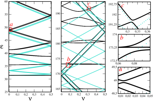
Figure 2: Color on-line. Dimensionless energies $\epsilon$ as a function of the magnetic flux $\nu$ for the annular cavity $\bf{S}$ with RSO coupling defined in the text. The spectrum for the concentric ring $d=0$ is plotted by turquoise open circles and for the eccentric QR, $d=0.05$, by black dotted lines. Left panel: Lowest eigenvalues. Central panel: Intermediate energy eigenvalues displaying avoided crossings for $d=0.05$. The regions inside the red boxes $a,b,c$ are enlarged in the right panels to show details of the avoided crossings.

When higher transverse channels are active, the spectrum for the eccentric QR is more involved. It displays additional avoided crossings generated by the mixing of levels that for $d=0$ were degenerated belonging to different transverse channels. Two detailed images of these avoided crossings are displayed in the right panel of Fig.2 in boxes $b$ and $c$.

Again, localized (flat levels) and current carrying states coexist in this region of the spectrum. As an example, in Fig.3 c) we plot for $\nu=0.2$ a contour plot of the probability amplitude for one of the angular localized states with $\epsilon=164.97$. In displays maxima and minima along the radial direction which are the fingerprint of basis states belonging to the second transverse channel of the concentric QR.

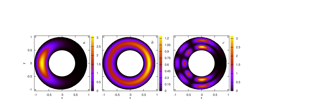
Figure 3: Contour plots of the probability amplitudes in the sample $S$ for $\nu=0.2$ and an eccentricity $d=0.05$. a) ground state with $\epsilon=26.96$, b) eigenstate with $\epsilon=49.11$ and c) eigenstate with $\epsilon=164.97$. The values of $\epsilon$ are given at $\nu=0$.

Taking into account that a given eigenspinor $\psi_{\epsilon_{i}}$ is an expansion in a basis of functions of total angular momentum, its probability amplitude has an angular profile which originates in the interference terms $\propto\sum_{m,m^{\prime}}\left(\varphi^{\uparrow}_{m-\nu}\varphi^{\uparrow}_{m^{\prime}-\nu}+{\varphi^{\downarrow}_{m-\nu+1}}\varphi^{\downarrow}_{m^{\prime}-\nu+1}\right)\cos(m-m^{\prime})\theta$ (see Eq.6). As we have shown in Fig.3, the angular profile depends on the specific eigenstate. This effect will also influence the spin accumulation describe in the next section.

III Spin accumulation effect

As a result of the RSO interaction, the spin projection is not a good quantum number. Given an eigenspinor $\psi_{\epsilon_{i}}$ whose general form is given by the Eq.6 the mean value of the z-projection of the spin density is proportional to

$$\sigma_{z}(\xi,\theta)=\psi_{\epsilon_{i}}^{\dagger}\hat{\sigma}_{z}\psi_{\epsilon_{i}}=\sum_{m=-M}^{M}\left(|\varphi^{\uparrow}_{m-\nu}|^{2}-|\varphi^{\downarrow}_{m-\nu+1}|^{2}\right)+$$

$$+2\sum_{m=-M}^{M}\sum_{m^{\prime}=m+1}^{M}\left(\varphi^{\uparrow}_{m-\nu}\varphi^{\uparrow}_{m^{\prime}-\nu}-{\varphi^{\downarrow}_{m-\nu+1}}\varphi^{\downarrow}_{m^{\prime}-\nu+1}\right)cos{((m-m^{\prime})\theta)}\;,$$ (13)

where we have used the fact that the radial part of the up and down components of an eigenspinor are real functions. Thus the products ${\varphi^{\uparrow,\downarrow}_{m-\nu}}\varphi^{\uparrow,\downarrow}_{m^{\prime}-\nu}$ are even under the interchange $m\leftrightarrow m^{\prime}$. The sum is for $-M\leq m\leq M$, where $M$ is given by the cut off in the expansion in the basis of total angular momentum eigenspinors.

In Ref.Lozano, Sanchez, 2005 it has been shown that in a multichannel concentric QR with RSO interaction, a spin accumulation effect (SAE) develops for finite values of the magnetic flux $\nu$. The SAE is the tendency of the total spin density for N particles, ${\Sigma}_{z}\equiv\sum_{N}\sigma_{z}$, to be different from zero, positive on one border of the sample and negative on the other one usaj and balseiro (2005).

In the concentric geometry and for $\nu=0$, states with opposite value of $j$ have opposite values of ${\sigma}_{z}\neq 0$ and then for even number of particles $N=2p$, is ${\Sigma}_{z}=0$. A finite $\nu\neq 0$ breaks the spatial symmetry between single particle states with opposite value of $j$. This can be understood in terms of the effective orbital index of the Bessel functions $m_{eff}\equiv m-\nu$, which turns to be $m-\nu$ and $-m-1-\nu$ for $j_{1}=m+1/2$ and $j_{2}=-j_{1}$, respectively. Thus the modulus of $m_{eff}$ decreases for $j_{1}$ and increases for $j_{2}$. As a consequence $\sigma_{z}$ is “pushed” toward the internal (external) boundary of the sample for the state label by $j_{1}$ ($j_{2}$). This is the main ingredient that contributes to generate the SAE in the concentric QRs Lozano, Sanchez (2005),i.e a total spin polarization $\Sigma_{z}$ that has opposite signs on each border of the sample $S$. However neither $\sigma_{z}$ nor $\Sigma_{z}$ depend on the angle $\theta$.

In the eccentric QR, the SAE develops an anisotropic angular profile due to the interference (last) term in Eq.LABEL:dsigma. The particular profile depends on the specific eigenspinor, exhibiting different characteristics for localized or current carrying states. As an example in Fig.4, we plot the contours plots of $\sigma_{z}(\xi,\theta)$ calculated for the three eigenspinors analyzed in Sec.II. The anisotropic angular pattern is clearly observed for the two localized states a) and c), where it is almost uniform for the current carrying state b).

Figure 4: Left panel:contour plot of the spin density $\sigma_{z}(\xi,\theta)$ for the three eigenspinors displayed in Fig.3. The anisotropic pattern in the angular direction is clearly observed for a) and c), where for panel b) the angular profile is almost uniform. The right panels show $\sigma_{z}$ vs $\xi$ for two specific angular directions selected in order to stress the effect. In all the cases is $\nu=0.2$.

As the particle number $N$ is increased to relevant experimental values, transverse channels are activated and the description of the effect becomes more involved. Nevertheless, mainly due to the existence of localized states along all energy ranges, the anisotropy in the SAE is a generic feature of the eccentric QR pierced by a magnetic flux.

As an illustration, in the left panels of Fig.5 we show the contour plots of the total spin density $\Sigma_{z}(\xi,\theta)\equiv\sum^{N}\sigma_{z}$ for $N=100$ particles and for two different values of the magnetic flux $\nu=0.2,0.45$.

The sensitivity of the SAE to the value of the magnetic flux $\nu$, is due to the qualitative changes that the eigenspinors experience at the avoided crossings in the flux-energy landscape. For this particular filling, the anisotropy in the SAE is more pronounced for $\nu=0.2$ than for $\nu=0.45$.

Besides the accumulation effect, the total spin density per unit area $M_{z}$, is different from zero and its value depends on $\theta$. Let the differential area be $dA=(b^{2}-a^{2})d\theta$ ($A=0.75\pi b^{2}$ is the area of sample $S$). It is easy to verify that $M_{z}(\theta)=\frac{4}{3}\int_{.5}^{1}\Sigma_{z}(\xi,\theta)\;\xi\;d\xi$. Taking $b=0.4\mu m$ and for $N=100$ particles, $M_{z}$ ranges from $M_{z}(\theta=0)=-0.3{\mu m}^{-2}$ to $M_{z}(\theta=100^{\circ})=0.48{\mu m}^{-2}$ for $\nu=0.2$. For $\nu=0.45$, $M_{z}$ is generally smaller, but the differences are still important and maxima between $M_{z}(\theta=0)=1.33\times 10^{-3}{\mu m}^{-2}$ and $M_{z}(\theta=180^{\circ})=-0.046{\mu m}^{-2}$. Thus, $M_{z}$ experiences important changes and even reverses it sign on distances of the order $1\mu m$. This is scketched in the right panels of Fig.5, where we show $\Sigma_{z}$ vs $\xi$ for the two angular directions $\theta$ especially selected to stress the anistropy.

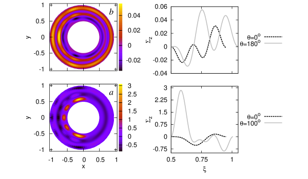
Figure 5: Left panels: Contour plot of the total spin density $\Sigma_{z}(\xi,\theta)$ for $N=100$ particles. Right panels: $\Sigma_{z}$ vs $\xi$ for the two angular directions $\theta$ selected to stress the anistropy. Lower (upper) panels correspond to $\nu=0.2$ ($\nu=0.45$).

IV Discussion and Summary

We have shown that a finite magnetic flux in an eccentric multichannel QR with SO interaction induces a spin accumulation effect (SAE) that exhibits an anisotropic profile in the angular direction. The effect, which is reminiscent to the drift of the spin polarization induced by the application of an in plane electric field, remains appreciable for filling numbers $(N\sim 100)$ which are experimentally realized in actual semiconductor QRs.

The spatial structure of the SAE which can be $\sim 1\mu m$ in the sample $S$ (see Fig.5), is not far from the sensitivity of detection methods based on scanning Kerr microscopy, which has been recently employed to image spin polarization in semiconductor channels Kato et  al. (2004); Crooker et al (2005).

In addition, the total spin density per unit area $M_{z}$, reaches at some angular directions, values $\sim 0.5{\mu m}^{-2}$. These values are comparable to the spin densities measured so far in the Spin Hall Effect in semiconductor channels Kato et  al. (2004).

In the presence of an external magnetic field perturbation, the spin magnetization should be proportional to $M_{z}$. With the help of new experimental techniques based on microresonators R. Deblock, R. Bel, B. Reulet, H. Bouchiat, D. Mailly (2002) or scanning magnetic force microscopes that can reach resolutions of $\sim 10nm$ magn08 , it should be feasible to sense differences in the values of $M_{z}$ bewteen sample regions separated $~{}1\mu m$.

We believe that our results could help to manipulate and functionalize the spin polarization in QRs with SO interaction, without using applied electric fields or external currents.

Partial financial support by ANPCyT Grants 06-483/03-13829 and CONICET are gratefully acknowledged. We would like to thank G. Usaj and C. Balseiro for helpful discussions.

References

- Awschalom et al. (2002) D. Awschalom, N. Samarth, and D. Loss, eds., Semiconductor Spintronics and Quantum Computation (Springer, New York, 2002).
- nitta, meijer and takayanagi (1999) J. Nitta, F.E Meijer and H. Takayanagi, Appl. Phys. Lett. 75, 695 (1999).
- aharonov and casher (1984) Y. Aharonovand A. Casher Phys. Rev. Lett. 53, 319 (1984).
- Berry (1984) M. V. Berry, Proc. R. Soc. London A 392, 45 (1984).
- Aronov and Lyanda? Geller (1993) A. G. Aronov and Y. B. Lyanda–Geller, Phys. Rev. Lett. 70, 343 (1993).
- Morpurgo et al (1998) A. F Morpurgo, J. P Heida, T.M Klapwijk and B.J van Wees,Phys. Rev. Lett. 80, 1050 (1998).
- Meijer et al. (2004) F. Meijer, A. Morpurgo, T. Klapwijk, T. Koga, and J. Nitta, Phys. Rev. B. 69, 035308 (2004).
- koning et al (2006) M. König, A. Tschetschetkin, E.M. Hankiewicz, J. Sinova,V. Hock,V. Daumer, M. Schäfer, C.R. Becker, H. Buhmann and L.W. Molenkamp, Phys. Rev. Lett. 96, 076804 (2006).
- Bergsten et al (2006) T. Bergsten, T. Kobayashi, Y. Sekine and J. Nitta, Phys. Rev. Lett. 97, 196803 (2006).
- meir gefen and entil-wohlman (1989) Y. Meir, Y. Gefen and O. Entil-Wohlman, Phys. Rev. Lett. 63, 798 (1989).
- loss and goldbart (1992) D. Loss and P. M. Goldbart, Phys. Rev. B. 45, 13544 (1992).
- Balatsky and Althsuler (1993) A. V. Balatsky and B. L. Althsuler, Phys. Rev. Lett. 70, 1678 (1993).
- Chaplik and Magarill (1995) A. V. Chaplik and L. I. MaGarill, Superlattices and Microstructures 18, 321 (1995).
- Splettstoesser, Governale and Zülicke (2002) J. Splettstoesser, M. Governale and U. Zülicke,Phys. Rev. B 68,165341 (2003).
- lobos and Aligia (2008) A.M. Lobos and A.A. Aligia Phys. Rev. Lett. 100, 016803 (2008).
- Lozano, Sanchez (2005) G.S. Lozanoand M. J. Sánchez Phys. Rev. B 72, 205315 (2005).
- Bychkov and Rashba (1984) Y. A. Bychkov and E. I. Rashba, JETP Letters 39, 78 (1984).
- Kato et al. (2004) Y.K Kato, R.C Myers, A.C Gossard and D.D Awschalom, Science 306, 1910 (2004).
- Sinova et al. (2004) J. Sinova, D. Culcer, Q. Niu, N. A. Sinitsyn, T. Jungwirth and A. H.MacDonald, Phys. Rev. Lett. 92, 126603 (2004).
- Wunderlich et al. (2005) J. Wunderlich,B. Kaestner, J. Sinova and T. Jungwirth, Phys. Rev. Lett. 94, 047204 (2005).
- usaj and balseiro (2005) G. Usaj and C.A Balseiro, Eur. Phys. Lett. 72, 631 (2005).
- (22) A. Reynoso, G. Usaj and C. A. Balseiro, Phys. Rev. B, 73, 115342, (2006).
- Bang Yau et al. (2002) Jeng-Bang Yau, E. P De Poortere and M. Shayegan, Phys. Rev. Lett. 88, 146801 (2002).
- grbic et al. (2007) B. Grbić,R. Leturcq, T. Ihn,K. Ensslin, D. Reuter and A.D. Wieck, Phys. Rev. Lett. 99, 176803 (2007).
- egydio, mijolaro (2004) R. Egydio de Carvalho and A.P. Mijolaro, Phys. Rev. B 70, 056212 (2004).
- bruno, latge (2005) A. Bruno-Alfonso and A. Latgé, Phys. Rev. B 71, 125312 (2005).
- Crooker et al (2005) S.A. Crooker, M. Furis ,X. Lou, , C. Adelmann ,D.L. Smith, C.J. Palmstrom ,P.A. Crowell, Science 309, 2191 (2005).
- singh, kothari (1984) G.S. Singh and L.S. Kothari, J. Math. Phys. 25, 810 (1984).
- R. Deblock, R. Bel, B. Reulet, H. Bouchiat, D. Mailly (2002) R. Deblock, R. Bel, B. Reulet, H. Bouchiat and D. Mailly, Phys. Rev. Lett. 89, 206803 (2002).
- (30) M. R. Koblischka, J. D. Wei, C. Richter, T. H. Sulzbach and U. Hartmann, Scanning 30, 27 (2008).