Topological Phases of Noncentrosymmetric Superconductors: Edge States, Majorana Fermions, and the Non-Abelian Statistics

Abstract

The existence of edge states and zero energy modes in vortex cores is a hallmark of topologically nontrivial phases realized in various condensed matter systems such as the fractional quantum Hall states, $p+ip$ superconductors, and ${\bm{Z}}_{2}$ insulators (quantum spin Hall state). We examine this scenario for two dimensional noncentrosymmetric superconductors which allow the parity-mixing of Cooper pairs. It is found that even when the $s$-wave pairing gap is nonzero, provided that the superconducting gap of spin-triplet pairs is larger than that of spin-singlet pairs, gapless edge states and zero energy Majorana modes in vortex cores emerge, characterizing topological order. Furthermore, it is shown that for Rashba superconductors, the quantum spin Hall effect produced by gapless edge states exists even under an applied magnetic field which breaks time-reversal symmetry provided that the field direction is perpendicular to the propagating direction of the edge modes. This result making a sharp contrast to the ${\bm{Z}}_{2}$ insulator is due to an accidental symmetry inherent in the Rashba model. It is also demonstrated that in the case with magnetic fields, the non-Abelian statistics of vortices is possible under a particular but realistic condition.

I Introduction

Topological phases of matter are quantum many-body states with topologically non-trivial structures of the Hilbert spaces Wen and Niu (1990). They are characterized by the existence of both topologically-protected gapless modes on the edges and a bulk energy gap which separates the ground state and excited states Wen (1990); Moore and Read (1991); Nayak and Wilczek (1996); Fradkin et al. (1998); Hatsugai (1993). Recently, topological phases are of interest in connection with wide ranges of subjects in condensed matter physics, such as the quantum Hall effect Thouless et al. (1982), $p+ip$ superconductors Moore and Read (1991); Nayak and Wilczek (1996); Fradkin et al. (1998); Read and Green (2000); Ivanov (2001); Stern et al. (2004), and ${\bm{Z}}_{2}$ topological insulators (quantum spin Hall effect) Kane and Mele (2005a); Sheng et al. (2005); Bernevig and Zhang (2006). The gapless edge states are topologically stable against the perturbations that do not break symmetries of systems, and play a crucial role in transport properties such as quantum (spin) Hall effects, which is, currently, inspiring applications to spintronics Wen (1990); Bernevig and Zhang (2006); Murakami et al. (2004). The total number of topologically-protected edge modes in a given system is associated with topological numbers, i.e. the TKNN number (the first Chern number of the U(1) bundle describing the many-body wave function) for systems without time-reversal symmetry Thouless et al. (1982); Hatsugai (1993), and the ${\bm{Z}}_{2}$ invariant (the parity of the spin-resolved TKNN number) for time-reversal invariant systems Kane and Mele (2005a).

The presence of low-energy edge modes also implies the fractionalization of quasiparticles in the bulk Lee et al. (2007). For instance, in a vortex core of a spinless $p+ip$ superconductor, there is a zero energy mode which is described by a Majorana fermion, i.e. a half of a conventional fermion Kopnin and Salomaa (1991). A vortex with a Majorana fermion is a quasiparticle obeying the non-Abelian statistics Read and Green (2000); Ivanov (2001); Sato (2003); Stone and Chung (2006); Stern et al. (2004): The braiding of vortices with Majorana fermions gives rise to the superposition of the degenerate many-body ground states. Owing to this entangled character, non-Abelian anyons can be utilized for the construction of fault-tolerant quantum computers Freedman et al. (2003); Stone and Chung (2006); Sarma et al. (2005); Tewari et al. (2007a); Nayak et al. . When there are odd number of vortices with Majorana fermions, the edge state must be also Majorana, since an isolated Majorana fermion is unphysical, and should be paired with another Majorana fermion Stone and Roy (2004). In this sense, the Majorana edge state is a concomitant of a zero energy Majorana mode in a vortex core, and the existence of both of them characterizes the topological order.

A more precise argument is given in terms of the low-energy effective theory. The low-energy effective theory for topological phases is the Chern-Simons theory, and both edge states and topological quasiparticles in the bulk are described by the corresponding conformal field theory. In the case with the level-$k$ SU(2) symmetry, it is the SU(2)_k Wess-Zumino-Witten theory, which is decomposed into the U(1) gaussian theory with the central charge $c=1$ and the ${\bm{Z}}_{k}$ parafermion theory with $c=\frac{2(k-1)}{k+2}$ Moore and Read (1991); Nayak and Wilczek (1996); Fradkin et al. (1998). For superconductors, where quasiparticles are superpositions of particles and holes, the U(1) gaussian part describing fractional charges for the fractional quantum Hall state is absent, and thus, the low-energy effective theory for edge states and quasiparticles is the ${\bm{Z}}_{k}$ parafermion theory. The topological phase of $p+ip$ superconductors corresponds to $k=2$, i.e. the Ising conformal field theory, the operator content of which includes Majorana fermions Stone and Chung (2006); Kitaev (2006).

The search for possible realization of topological phases is an intriguing and challenging issue involving the development of novel concepts for quantum condensed states as well as potential technological applications. In this paper, we demonstrate that two dimensional (2D) noncentrosymmetric superconductors (NCS) under certain circumstances provide another candidate for the physical realization of a topological phase, which supports the existence of edge states and zero energy modes in vortex cores. In NCS, asymmetric spin-orbit (SO) interactions play crucial roles in various exotic superconducting phenomena such as parity-mixing of Cooper pairs, magnetoelectric effects, and helical vortex phases Edelstein (1989, 1995); Gor’kov and Rashba (2001); Yip (2002); Frigeri et al. (2004); Samokhin (2004); Kaur et al. (2005); Fujimoto (2005, 2007a). It is found that the asymmetric SO interaction is also a key to realize topological phases in NCS. We investigate the edge states and the zero energy vortex core states in NCS by using both numerical and analytical methods, and verify the condition for the realization of topological phases in NCS.

The main results of this paper are as follows. For 2D NCS with the admixture of $s$-wave pairing and $p$-wave pairing, as long as the $p$-wave gap is larger than the $s$-wave gap, topological phases are realized. The classification of the topological phases in NCS is completed by examining topological numbers. In the absence of magnetic fields, a ${\bm{Z}}_{2}$ topological phase with two gapless edge modes emerges, which leads to the quantum spin Hall effect; i.e. when an electric field or a temperature gradient is applied, a spin Hall current carried by the edge state flows in the direction perpendicular to the applied external field. Moreover, it is shown that in the case of the Rashba SO interaction, the gapless edge modes are stable against weak magnetic field applied perpendicular to the direction in which the edge modes propagate. This is a bit surprising because the magnetic field which breaks time-reversal symmetry flaws the ${\bm{Z}}_{2}$ classification of the topological phase, and also the TKNN number is still zero for such a weak magnetic field. In fact, the stability of this topological phase is due to an accidental symmetry for particular symmetry points in the Brillouin Zone specific to the Rashba model, which is characterized by another topological number, “winding number”. We will clarify the condition for the nonzero winding number in this paper. In addition to these spin Hall states, there is also a topological phase with the nonzero TKNN number, which is analogous to the quantum Hall state, and realized for a particular electron density with a magnetic field. The implication of these gapless edge states for experimental observations will be also discussed.

Furthermore, we examine the vortex core state for these topological phases by solving the Bogoliubov-de Gennes equations. On the basis of both numerical and analytical methods, it is found that zero energy Majorana fermion modes exist in the vortex cores. It is also verified how the non-Abelian statistics of vortices is realized in NCS. The non-Abelian statistics of vortices in superconductors has been considered so far for the chiral $p+ip$ state.Read and Green (2000); Ivanov (2001) In the case of spinless $p+ip$ state, there is only one zero energy Majorana mode in a vortex, which is a non-Abelian anyon. In the case of spinful $p+ip$ state, there are two Majorana fermions in a vortex corresponding to spin up and spin down states, which form a usual complex fermion. The non-Abelian statistics is not realized for this situation. As Ivanov elucidated, when there is a half quantum vortex which suppresses one of two Majorana fermions in a vortex core, vortices behave as non-Abelian anyons Ivanov (2001). For NCS, however, this scenario is not applicable, because the half-quantum vortex is a texture of the $d$-vector of $p$-wave pairing, and the $d$-vector in NCS is locked by the strong SO interaction. As proposed by one of the authors Fujimoto (2008), when one tunes a chemical potential so as that the Fermi level crosses the $\Gamma$ point in the Brillouin zone at which the electron band is a Dirac cone, and applies a Zeeman field parallel to the $z$-direction, a Majorana fermion associated with the Dirac cone is eliminated, and only one Majorana fermion survives in a vortex core, which makes the non-Abelian statistics of vortices possible. We examine this strategy by using an analytical approach based on the index theorem for zero modes developed by Tewari, Sarma and Lee in the case of $p+ip$ superconductors Tewari et al. (2007b). It is found that when the spin-triplet gap is larger than the spin-singlet gap, the non-Abelian statistics of vortices is realized for the situation mentioned above.

It would be useful to comment on some recent other studies related to the present paper. 1) Some topological properties of the Rashba type NCS, such as the nodal structure of the gap function and the edge state, were discussed in Sato (2006); Tanaka et al. . While these literatures assumed the time-reversal symmetry and were based on the ${\bm{Z}}_{2}$ topological number, we complete the topological classification by taking into account the TKNN number simultaneously. We also find that the “winding number” mentioned above is useful to characterize topological phases of the Rashba superconductors. 2) In Fujimoto (2008), a possibility of zero energy states in vortex cores for purely $s$-wave noncentrosymmetric superconductors under strong magnetic fields was suggested. Later, unfortunately, it was turned out that the zero energy vortex core state found in Fujimoto (2008) is spurious, and there is no zero energy state in purely s-wave cases. The misleading conclusion in Fujimoto (2008) is due to the erroneous assumption that the unitary transformation which diagonalizes the spin index is commutative with the center of mass coordinate of Cooper pairs raised by the presence of vortices. This assumption is valid only when the quasiclassical approximation is justified. This is not the case for the issue of zero energy vortex core states. This point will be discussed in more detail in Sec. IV.2 of the current paper. 3) Independently, Lu and Yip elucidated that in NCS with parity-mixing, the zero energy vortex core state is possible only when the gap of the spin-triplet pairs is larger than that of the spin-singlet pairs Lu and Yip . They examined the condition for zero energy modes of the Bogoliubov-de Gennes (BdG) equations without obtaining explicit solutions. However, to investigate the possible realization of the non-Abelian statistics of vortices, it is desirable to derive the explicit zero energy solutions which enable us to see whether a zero energy mode in a vortex core is a Majorana fermion or a usual complex fermion. This issue is addressed in the current paper.

The organization of this paper is as follows. In Sec. II, we start with a general topological argument, which enables us to understand edge and vortex core states clearly, providing the complete classification of topological phases in NCS. In Sec. III, gapless edge states in NCS are investigated by using the general topological argument and numerical methods. The implication for transport properties associated with edge states is also discussed. In Sec. IV, we explore zero energy vortex core states for NCS on the basis of numerical solutions for the Bogoliubov-de Gennes equations and an analytical approach based on the index theorem for zero energy states, and clarify the condition for the realization of the non-Abelian statistics of vortices. We conclude in Sec. V with a summary of our results.

II Topological numbers for noncentrosymmetric superconductors

In this paper, we consider type II NCS with Rashba-type SO interaction Rashba (1960) in two dimensions. For concreteness, we define our model on the square lattice, though the following argument does not rely on the particular choice of the crystal structure. Then the model Hamiltonian is

$${\mathcal{H}} = \sum_{{\bm{k}},\sigma}\varepsilon_{\bm{k}}c_{{\bm{k}}\sigma}^{\dagger}c_{{\bm{k}}\sigma}-\mu_{\rm B}H_{z}\sum_{{\bm{k}},\sigma}(\sigma_{z})_{\sigma\sigma^{\prime}}c_{{\bm{k}}\sigma}^{\dagger}c_{{\bm{k}}\sigma}+\alpha\sum_{{\bm{k}},\sigma,\sigma^{\prime}}{\bm{\mathcal{L}}}_{0}({\bm{k}})\cdot{\bm{\sigma}}_{\sigma\sigma^{\prime}}c_{{\bm{k}}\sigma}^{\dagger}c_{{\bm{k}}\sigma^{\prime}}$$ (1)

$$+ \frac{1}{2}\sum_{{\bm{k}}\sigma\sigma^{\prime}}\Delta_{\sigma\sigma^{\prime}}({\bm{k}})c_{{\bm{k}}\sigma}^{\dagger}c_{-{\bm{k}}\sigma^{\prime}}^{\dagger}+\frac{1}{2}\sum_{{\bm{k}}\sigma\sigma^{\prime}}\Delta_{\sigma^{\prime}\sigma}^{*}({\bm{k}})c_{-{\bm{k}}\sigma}c_{{\bm{k}}\sigma^{\prime}},$$

where $c_{{\bm{k}}\sigma}^{\dagger}$ ($c_{{\bm{k}}\sigma}$) is a creation (an annihilation) operator for an electron with momentum ${\bm{k}}=(k_{x},k_{y})$, spin $\sigma$. The energy band dispersion is $\varepsilon_{\bm{k}}=-2t(\cos k_{x}+\cos k_{y})-\mu$ with the hopping parameter $t$ and the chemical potential $\mu$, and the Rashba SO coupling is ${\bm{\mathcal{L}}}_{0}({\bm{k}})=(\sin k_{y},-\sin k_{x})$. For simplicity, we assume that $t>0$ and $\mu<0$. Because of parity mixing of Cooper pairs, the gap function $\Delta({\bm{k}})$ has both a spin-triplet component ${\bm{d}}({\bm{k}})$ and a spin-singlet one $\psi({\bm{k}})$ at the same time, $\Delta({\bm{k}})=i\psi({\bm{k}})\sigma_{y}+i{\bm{d}}({\bm{k}}){\bm{\sigma}}\sigma_{y}$. Due to the strong SO coupling, the spin-triplet component ${\bm{d}}({\bm{k}})$ is aligned with the Rashba coupling, ${\bm{d}}({\bm{k}})=\Delta_{\rm t}{\bm{\mathcal{L}}_{0}}({\bm{k}})$ Frigeri et al. (2004). For the spin-singlet component $\psi$, we assume a $s$-wave pairing, $\psi({\bm{k}})=\Delta_{\rm s}$. The amplitudes $\Delta_{\rm t,s}$ are chosen as real. The Zeeman coupling $\mu_{\rm B}H_{z}\sum_{\bm{k}}(c^{\dagger}_{{\bm{k}}\uparrow}c_{{\bm{k}}\uparrow}-c^{\dagger}_{{\bm{k}}\downarrow}c_{{\bm{k}}\downarrow})$ with $H_{z}$ a magnetic field in the $z$ direction has been also introduced for later use.

Before going to study topological properties of the system, we first examine the bulk spectrum of the system. Topological nature of the system changes only when the gap of the bulk spectrum closes. The bulk spectrum $E({\bm{k}})$ of the system is obtained by diagonalizing the following matrix,

$$H({\bm{k}})=\left(\begin{array}[]{cc}\varepsilon_{\bm{k}}-\mu_{\rm B}H_{z}\sigma_{z}+\alpha{\bm{\mathcal{L}}}_{0}({\bm{k}})\cdot{\bm{\sigma}}&i\Delta_{\rm s}\sigma_{y}+i\Delta_{\rm t}{\bm{\mathcal{L}}}_{0}({\bm{k}})\cdot{\bm{\sigma}}\sigma_{y}\\ -i\Delta_{\rm s}\sigma_{y}-i\Delta_{\rm t}{\bm{\mathcal{L}}}_{0}({\bm{k}})\sigma_{y}\cdot{\bm{\sigma}}&-\varepsilon_{\bm{k}}+\mu_{\rm B}H_{z}\sigma_{z}+\alpha{\bm{\mathcal{L}}}_{0}({\bm{k}})\cdot{\bm{\sigma}}^{*}\end{array}\right),$$ (4)

and we have

$$E({\bm{k}})=\pm\sqrt{\varepsilon_{\bm{k}}^{2}+(\alpha^{2}+\Delta_{\rm t}^{2}){\bm{\mathcal{L}}}_{0}({\bm{k}})^{2}+\mu_{\rm B}^{2}H_{z}^{2}+\Delta_{\rm s}^{2}\pm 2\sqrt{(\varepsilon_{\bm{k}}\alpha+\Delta_{\rm s}\Delta_{\rm t})^{2}{\bm{\mathcal{L}}}_{0}({\bm{k}})^{2}+(\varepsilon_{\bm{k}}^{2}+\Delta_{\rm s}^{2})\mu_{\rm B}^{2}H_{z}^{2}}}.$$ (5)

The gap of the system closes only when

$$\varepsilon_{\bm{k}}^{2}+(\alpha^{2}+\Delta_{\rm t}^{2}){\bm{\mathcal{L}}}_{0}({\bm{k}})^{2}+\mu_{\rm B}^{2}H_{z}^{2}+\Delta_{\rm s}^{2}=2\sqrt{(\varepsilon_{\bm{k}}\alpha+\Delta_{\rm s}\Delta_{\rm t})^{2}{\bm{\mathcal{L}}}_{0}({\bm{k}})^{2}+(\varepsilon_{\bm{k}}^{2}+\Delta_{\rm s}^{2})\mu_{\rm B}^{2}H_{z}^{2}},$$ (6)

which is equivalent to

$$\varepsilon_{\bm{k}}^{2}+\Delta_{\rm s}^{2}=\mu_{\rm B}^{2}H_{z}^{2}+(\alpha^{2}+\Delta_{\rm t}^{2}){\bm{\mathcal{L}}}_{0}({\bm{k}})^{2},\quad\varepsilon_{\bm{k}}\Delta_{\rm t}{\bm{\mathcal{L}}}_{0}({\bm{k}})=\Delta_{\rm s}\alpha{\bm{\mathcal{L}}}_{0}({\bm{k}}).$$ (7)

When $\Delta_{\rm t}\neq 0$, (7) is met either when

$$\varepsilon_{\bm{k}}=\frac{\Delta_{\rm s}}{\Delta_{\rm t}}\alpha,\quad\left(1+\frac{\alpha^{2}}{\Delta_{\rm t}^{2}}\right)\left(\Delta_{\rm t}^{2}{\bm{\mathcal{L}}}_{0}({\bm{k}})^{2}-\Delta_{\rm s}^{2}\right)+\mu_{\rm B}^{2}H_{z}^{2}=0.$$ (8)

or

$$\varepsilon_{\bm{k}}^{2}+\Delta_{s}^{2}=\mu_{\rm B}^{2}H_{z}^{2},\quad{\bm{\mathcal{L}}}_{0}({\bm{k}})=0.$$ (9)

In the absence of the magnetic field, only Eqs.(8) can be met and they are rewritten in simpler forms,

$$\varepsilon_{\bm{k}}^{2}=\alpha^{2}{\bm{\mathcal{L}}}_{0}({\bm{k}})^{2},\quad\Delta_{\rm t}^{2}{\bm{\mathcal{L}}}_{0}({\bm{k}})^{2}=\Delta_{\rm s}^{2}.$$ (10)

Topological nature of the system does not change unless (8) or (9) (or (10) when $H_{z}=0$) is satisfied.

II.1 ${\bm{Z}}_{2}$ topological number

When $H_{z}=0$, the system is time-reversal invariant, and the topological property is characterized by the ${\bm{Z}}_{2}$ invariant Kane and Mele (2005a, b); Moore and Balents (2007); Fu et al. (2007); Roy (a); Fu and Kane (2007), . We will show that if the spin-triplet pairing is stronger than the spin-singlet one, the ${\bm{Z}}_{2}$ number is non-trivial.

To calculate the ${\bm{Z}}_{2}$ number, we adiabatically deform the Hamiltonian of the system without gap closing. This process does not change the ${\bm{Z}}_{2}$ topological number, since it changes only when the gap closes. From (10), it is found that if the spin-triplet amplitude $\Delta_{\rm t}{\bm{\mathcal{L}}}_{0}({\bm{k}})$ is larger than the spin-singlet one $\Delta_{\rm s}$ on the Fermi surface given by $\varepsilon_{\bm{k}}=\alpha{\bm{\mathcal{L}}}_{0}({\bm{k}})$, we can take $\Delta_{\rm s}\rightarrow 0$, then $\alpha\rightarrow 0$ without gap closing. (If $\varepsilon_{\bm{k}}=0$ at one of the time-reversal momenta ${\bm{k}}=(0,0),(\pi,0),(0,\pi),(\pi,\pi)$, the gap closes when $\Delta_{\rm s}=0$. However, this undesirable gap closing can be avoided by changing $\mu$ or $t$ slightly.) Thus, its ${\bm{Z}}_{2}$ number is the same as that of the pure spin-triplet SC with ${\bm{d}}({\bm{k}})=\Delta_{\rm t}{\bm{\mathcal{L}}}_{0}({\bm{k}})$.

As was shown in Sato , the ${\bm{Z}}_{2}$ topological number $(-1)^{\nu}$ for a pure spin-triplet SC is determined by its dispersion $\varepsilon_{\bm{k}}$ in the normal state,

$$(-1)^{\nu}=\prod_{{\bm{k}}=(0,0),(0,\pi),(\pi,0),(\pi,\pi)}{\rm sgn}\varepsilon_{\bm{k}}.$$ (11)

From this formula, it is easily shown that the ${\bm{Z}}_{2}$ number is always non-zero (mod 2) for the square lattice system. Therefore, from the argument above, if the spin-triplet pairing is stronger than the singlet one, the NCS is a topological insulator with a non-trivial ${\bm{Z}}_{2}$ number. This topological superconductor belongs to the same class as one discussed in Qi et al. ; Roy (b); Tanaka et al. .

II.2 TKNN number

In the presence of a magnetic field, the time-reversal invariance is broken. The ${\bm{Z}}_{2}$ topological number is no longer meaningful, and the TKNN number plays a central role in topological nature of the system instead. In the following argument, we consider only the Zeeman effect of the magnetic field, neglecting the orbital depairing effect. When the energy scale of the SO interaction is sufficiently larger than the Zeeman energy scale, the Pauli depairing effect does not exit for magnetic fields parallel to the $z$-axis, and the structure of the ${\bm{d}}$-vector for the spin-triplet pairs is not affected by the Zeeman effect Frigeri et al. (2004); Fujimoto (2007a). We assume such situations. The effect of the orbital depairing effect will be discussed at the end of this subsection.

In order to obtain a non-zero TKNN number, the magnetic field should be large enough to have a gap closing. Otherwise the TKNN number must be zero since the system is adiabatically connected to the case with $H_{z}=0$. (When $H_{z}=0$, the TKNN number becomes zero because of time-reversal invariance.) When the spin-triplet pairing is stronger than the singlet one, (8) is never met in the presence of the magnetic field, and a gap closing occurs only when (9) is satisfied. Since ${\bm{\mathcal{L}}}_{0}({\bm{k}})$ is zero at ${\bm{k}}=(0,0),(0,\pi),(\pi,0),(\pi,\pi)$, it is found that we have a gap closing if one of the following equations is satisfied,

$$(-4t-\mu)^{2}+\Delta_{\rm s}^{2}=\mu_{\rm B}^{2}H_{z}^{2},\quad\mu^{2}+\Delta_{\rm s}^{2}=\mu_{\rm B}^{2}H_{z}^{2},\quad(4t-\mu)^{2}+\Delta_{\rm s}^{2}=\mu_{\rm B}^{2}H_{z}^{2}.$$ (12)

From this, it is found that we have a two classes of phase diagram illustrated in Fig.1. a) For $-4t<\mu<-2t$, the first phase transition occurs at $\mu_{\rm B}H_{z}=\sqrt{(4t+\mu)^{2}+\Delta_{\rm s}^{2}}$, and the second one at $\mu_{\rm B}H_{z}=\sqrt{\mu^{2}+\Delta_{\rm s}^{2}}$, and the third one at $\mu_{\rm B}H_{z}=\sqrt{(4t-\mu)^{2}+\Delta_{\rm s}^{2}}$. b) For $-2t<\mu<0$, the first phase transition occurs at $\mu_{\rm B}H_{z}=\sqrt{\mu^{2}+\Delta_{\rm s}^{2}}$, and the second one at $\mu_{\rm B}H_{z}=\sqrt{(4t+\mu)^{2}+\Delta_{\rm s}^{2}}$, and the third one at $\mu_{\rm B}H_{z}=\sqrt{(4t-\mu)^{2}+\Delta_{\rm s}^{2}}$. The patterns of the TKNN numbers differ for these parameter regions.

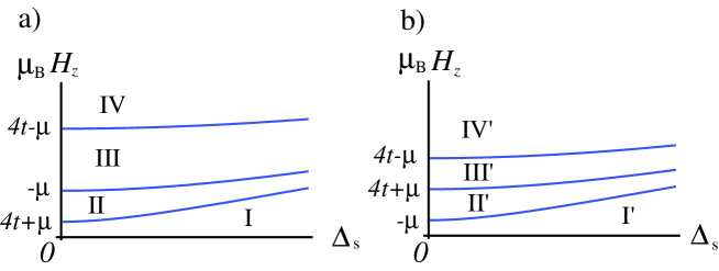
Figure 1: Schematic picture of phase diagram of 2D NCS with Rashba coupling.

The TKNN number for each phase is evaluated by using the adiabatic deformation of the Hamiltonian in a similar manner as Sec.II.1. As is evident from Fig.1, we can take $\Delta_{\rm s}=\alpha=0$ without crossing the phase boundary. For $\Delta_{\rm s}=\alpha=0$, the up-spin electron and down-spin electron are decoupled from each other, and the Hamiltonian reduces to a pair of $2\times 2$ matrices,

$$H_{\uparrow\uparrow}({\bm{k}})=\left(\begin{array}[]{cc}\varepsilon_{\bm{k}}-\mu_{\rm B}H_{z}&-i\Delta_{\rm t}(\sin k_{x}-i\sin k_{y})\\ i\Delta_{\rm t}(\sin k_{x}+i\sin k_{y})&-\varepsilon_{\bm{k}}+\mu_{\rm B}H_{z}\end{array}\right),$$ (15)

$$H_{\downarrow\downarrow}({\bm{k}})=\left(\begin{array}[]{cc}\varepsilon_{\bm{k}}+\mu_{\rm B}H_{z}&-i\Delta_{\rm t}(\sin k_{x}+i\sin k_{y})\\ i\Delta_{\rm t}(\sin k_{x}-i\sin k_{y})&-\varepsilon_{\bm{k}}-\mu_{\rm B}H_{z}\end{array}\right).$$ (18)

Using these $2\times 2$ matrices, we can evaluate the TKNN integers. By rewriting $H_{\sigma\sigma}({\bm{k}})$ $(\sigma=\uparrow,\downarrow)$ as $H_{\sigma\sigma}({\bm{k}})={\bm{R}}_{\sigma}({\bm{k}})\cdot{\bm{\sigma}}$, the TKNN number $I_{\rm TKNN}$ is given by

$$I_{\rm TKNN}=-\sum_{\sigma}\frac{1}{8\pi}\int\int d^{2}{\bm{k}}\epsilon_{abc}\epsilon_{ij}\hat{\bm{R}}_{\sigma}^{a}\partial_{i}\hat{\bm{R}}_{\sigma}^{b}\partial_{j}\hat{\bm{R}}_{\sigma}^{c},$$ (19)

with $\hat{\bm{R}}_{\sigma}={\bm{R}}_{\sigma}/|{\bm{R}}_{\sigma}|$.

In Table.1, we summarize the obtained TKNN numbers. The phases IV and IV’ are trivial band insulators, and of no interest. The other phases are in topologically nontrivial states. For the phases II, III, and III’, there is only one band which crosses the Fermi level, and is associated with the nonzero TKNN number. The sign of the TKNN number depends on the curvature of the Fermi surface as well as the chirality of the gap function, since it is related to the Hall conductivity. The gap functions for the phases II, III, and III’ possess the same chirality, and hence, for the positive curvature of the Fermi surface, $I_{\rm TKNN}>0$ (the phase II), and for the negative curvature, $I_{\rm TKNN}<0$ (the phases III and III’). In the phase II’, there are two bands with opposite signs of the curvatures of the Fermi surfaces. Also, the gap functions for these bands have opposite chiralities. Thus, each of the two bands contributes to the TKNN number equal to $-1$, leading to the total TKNN number $I_{\rm TKNN}=-2$. The phases II, III, II’, and III’ are analogous to the quantum Hall state.

For the phases I and I’, although both the TKNN number and the ${\bm{Z}}_{2}$ index are zero, there exist topological orders with two gapless edge modes and Majorana fermions in vortex cores, as will be shown in Sec. III and Sec. IV, and their topological nature is similar to that of the ${\bm{Z}}_{2}$ insulator. In the next subsection, it will be clarified that these phases are characterized by another topological number, i.e. winding number.

In the argument above, the orbital depairing effect of magnetic fields is ignored. For typical superconductors, the orbital limiting field is $H_{\rm c}^{\rm orb}\sim E_{F}(\Delta/E_{F})^{2}/\mu_{\rm B}\ll t/\mu_{\rm B}$ with the Fermi energy $E_{F}$. Thus, superconductivity does not survive in the strong magnetic field regions, III and III’, though the Pauli depairing effect is completely suppressed by the strong asymmetric SO interaction as mentioned before. (To avoid confusion, we would like to stress again that the topological phases obtained above by putting $\alpha=0$ can be deformed into topologically equivalent states with nonzero large $\alpha$, unless the bulk gap closes.) On the other hand, the realization of the phases I, II, I’, and II’ in the weak field regions is feasible.

a) $-4t\leq\mu<-2t$
	$\mu_{\rm B}H_{z}$	$I_{\rm TKNN}$	$I(0)$	$I(\pi)$
I	$0<\mu_{\rm B}H_{z}<\sqrt{(4t+\mu)^{2}+\Delta_{s}^{2}}$	0	-2	0
II	$\sqrt{(4t+\mu)^{2}+\Delta_{s}^{2}}<\mu_{\rm B}H_{z}<\sqrt{\mu^{2}+\Delta_{s}^{2}}$	1	-1	0
III	$\sqrt{\mu^{2}+\Delta_{s}^{2}}<\mu_{\rm B}H_{z}<\sqrt{(4t-\mu)^{2}+\Delta_{s}^{2}}$	-1	0	-1
IV	$\sqrt{(4t-\mu)^{2}+\Delta_{s}^{2}}<\mu_{\rm B}H_{z}$	0	0	0

b) $-2t<\mu<0$
	$\mu_{\rm B}H_{z}$	$I_{\rm TKNN}$	$I(0)$	$I(\pi)$
I’	$0<\mu_{\rm B}H_{z}<\sqrt{\mu^{2}+\Delta_{s}^{2}}$	0	-2	0
II’	$\sqrt{\mu^{2}+\Delta_{s}^{2}}<\mu_{\rm B}H_{z}<\sqrt{(4t+\mu)^{2}+\Delta_{s}^{2}}$	-2	-1	-1
III’	$\sqrt{(4t+\mu)^{2}+\Delta_{s}^{2}}<\mu_{\rm B}H_{z}<\sqrt{(4t-\mu)^{2}+\Delta_{s}^{2}}$	-1	0	-1
IV’	$\sqrt{(4t-\mu)^{2}+\Delta_{s}^{2}}<\mu_{\rm B}H_{z}$	0	0	0

Table 1: The TKNN integer $I_{\rm TKNN}$ and the winding number $I(k_{y})$ for 2D NCS with Rashba coupling.

II.3 Winding number

As was mentioned in the previous subsection, the NCS with the Rashba coupling has an additional topological number, in addition to the ${\bm{Z}}_{2}$ and TKNN numbers. Unlike the usual topological number, the additional topological number is defined only for particular values of momentum, but it is also useful to understand properties of edge states and vortex core states, which are specific to the 2D NCS, in the presence of a magnetic field.

To define the topological number, let us consider the particle-hole symmetry of the Hamiltonian,

$$\Gamma H({\bm{k}})\Gamma^{\dagger}=-H(-{\bm{k}})^{*},\quad\Gamma=\left(\begin{array}[]{cc}0&{\bm{1}}\\ {\bm{1}}&0\end{array}\right).$$ (22)

For $k_{y}=0$ or $k_{y}=\pi$, we have $H(-{\bm{k}})^{*}=H({\bm{k}})$, thus the Hamiltonian anti-commutes with $\Gamma$, $\{\Gamma,H({\bm{k}})\}=0.$ This implies that if we take the basis where $\Gamma$ is diagonal $\Gamma={\rm diag}(1,1,-1,-1)$, then the Hamiltonian becomes off-diagonal

$$H({\bm{k}})=\left(\begin{array}[]{cc}0&q({\bm{k}})\\ q^{\dagger}({\bm{k}})&0\end{array}\right),$$ (25)

for these values of $k_{y}$. Using $q({\bm{k}})$, we can define the topological number as Wen and Zee (1989),

$$I(k_{y})=\frac{1}{4\pi i}\int_{-\pi}^{\pi}dk_{x}{\rm tr}(q^{-1}({\bm{k}})\partial_{k_{x}}q({\bm{k}})-q^{\dagger-1}({\bm{k}})\partial_{k_{x}}q^{\dagger}({\bm{k}})),\quad(k_{y}=0,\,\pi).$$ (26)

An explicit calculation shows that $q({\bm{k}})$ is given by

$$q({\bm{k}})=\left(\begin{array}[]{cc}\varepsilon_{\bm{k}}-\mu_{\rm B}H_{z}+i\Delta_{\rm t}\sin k_{x}&-\Delta_{\rm s}+i\alpha\sin k_{x}\\ \Delta_{\rm s}-i\alpha\sin k_{x}&\varepsilon_{\bm{k}}+\mu_{\rm B}H_{z}+i\Delta_{\rm t}\sin k_{x}\end{array}\right).$$ (29)

From this, we can calculate $I(k_{y})$ $(k_{y}=0,\pi)$ for each phase in Fig.1. The result is summarized in Table.1.

The additional topological number $I(k_{y})$ is accidental and very sensitive to the direction of the magnetic field. While $I(k_{y})$ remains well-defined even in the presence of a magnetic field in the $x$-direction, it becomes meaningless if we apply a magnetic field in the $y$-direction, $H_{y}$, since $H_{y}$ breaks the relation $H(-{\bm{k}})^{*}=H({\bm{k}})$ for $k_{y}=0,\pi$. From the bulk-edge correspondence, this means that edge states for Rashba type NCS are also very sensitive to the direction of the magnetic field, which will be confirmed numerically in the next section.

III Edge states in noncentrosymmetric superconductors

In this section, we investigate edge states for the 2D NCS numerically. From the bulk edge correspondence, a non-trivial bulk topological number implies gapless edge states. This will be confirmed in this section. Experimental implications for the gapless edge states are also discussed in Sec.III.3.

III.1 Without a magnetic field

Let us first study edge states for the 2D NCS in the absence of magnetic field. Consider the lattice version of the Hamiltonian (1)

$${\cal H} = -t\sum_{\langle{\bm{i}},{\bm{j}}\rangle,\sigma}c_{{\bm{i}}\sigma}^{\dagger}c_{{\bm{j}}\sigma}-\mu\sum_{{\bm{i}},\sigma}c_{{\bm{i}}\sigma}^{\dagger}c_{{\bm{i}}\sigma}-\mu_{\rm B}H_{z}\sum_{{\bm{i}},\sigma,\sigma^{\prime}}(\sigma_{z})_{\sigma\sigma^{\prime}}c_{{\bm{i}}\sigma}^{\dagger}c_{{\bm{i}}\sigma^{\prime}}-i\frac{\alpha}{2}\sum_{\langle{\bm{i}},{\bm{j}}\rangle,\sigma,\sigma^{\prime}}({\bm{\sigma}}_{\sigma\sigma^{\prime}}\times\hat{\bm{r}}_{{\bm{i}}{\bm{j}}})_{z}c_{{\bm{i}}\sigma}^{\dagger}c_{{\bm{j}}\sigma^{\prime}}$$ (30)

$$+\Delta_{\rm s}\sum_{\bm{i}}(c_{{\bm{i}}\uparrow}^{\dagger}c_{{\bm{i}}\downarrow}^{\dagger}+{\rm h.c.})$$

$$-\frac{1}{2}\Delta_{\rm t}\sum_{\bm{i}}(c_{{\bm{i}}\uparrow}^{\dagger}c_{{\bm{i}}+\hat{x}\uparrow}^{\dagger}+c_{{\bm{i}}\downarrow}^{\dagger}c_{{\bm{i}}+\hat{x}\downarrow}^{\dagger}-ic_{{\bm{i}}\uparrow}^{\dagger}c_{{\bm{i}}+\hat{y}\uparrow}^{\dagger}+ic_{{\bm{i}}\downarrow}^{\dagger}c_{{\bm{i}}+\hat{y}\downarrow}^{\dagger}+{\rm h.c.}),$$

where ${\bm{i}}=(i_{x},i_{y})$ denotes a site on the square lattice, $\hat{\bm{r}}_{{\bm{i}}{\bm{j}}}$ a unit vector from a site ${\bm{i}}$ to a site ${\bm{j}}$. The sum $\sum_{\langle{\bm{i}}{\bm{j}}\rangle}$ is taken between the nearest neighbor sites. In this subsection, we suppose $H_{z}=0$. Consider the system with two edges at $i_{x}=0$ and $i_{x}=N_{x}$, and put the periodic boundary condition in the $y$ direction. By solving numerically the energy spectrum as a function of the momentum $k_{y}$ in the $y$ direction, edge states for NCS are studied.

As was shown in the previous section, the ${\bm{Z}}_{2}$ topological number is non-zero if the gap of the spin-triplet pairs are larger than that of the singlet. Therefore, from the bulk-edge correspondence, there should always exist gapless edges if the spin-triplet pairs dominates the superconductivity. In Fig.2 a), we show the energy spectrum of the 2D NCS with edges. It is found that there exist gapless edge states in the bulk gap. The gapless edges states form a Kramers pair.

For comparison, we also illustrate the energy spectrum for the 2D NCS with purely $s$-wave paring in Fig.2 b). As is seen clearly, no edge state is obtained. This is also consistent with the trivial ${\bm{Z}}_{2}$ number of the purely $s$-wave paring.

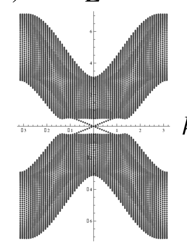
Figure 2: The energy spectra of the 2D NCS with edges at $i_{x}=0$ and $i_{x}=50$ in the absence of magnetic field. Here $k_{y}$ denotes the momentum in the $y$-direction. We take $t=1$, $\mu=-3$, $\alpha=0.6$. a) NCS with dominating $p$-wave paring. $\Delta_{\rm t}=0.6$ and $\Delta_{\rm s}=0.1$. b) NCS with purely $s$-wave paring. $\Delta_{\rm t}=0$ and $\Delta_{\rm s}=0.6$.

III.2 With a magnetic field

Let us now examine edge states in the case with a magnetic field. As is shown in the previous section, there exists a variety of topological phases characterized by the topological numbers.

In Figs.3 and 4, we illustrate the energy spectra of 2D NCS with edges for various topological phases. All phases have a bulk gap, and some of them have gapless edge states corresponding to the non-trivial topological numbers in Table 1. It is found that for $k_{y}$ with nonzero $I(k_{y})$ $(k_{y}=0,\pi)$, a zero energy edge state always appears, and the number of zero energy edge states coincides with the absolute value of $I(k_{y})$. We also find that a phase with a non-zero $I_{\rm TKNN}$ has a edge state with the total chirality $I_{\rm TKNN}$. These results are also consistent with the bulk-edge correspondence.

We also notice that the gapless edge states in the phases I and I’ are very sensitive to the direction of the applied magnetic field. As seen in Fig.5, while the gapless edge states are stable under a magnetic field in the $x$-direction, they become unstable under a small magnetic field in the $y$-direction. This behavior is naturally understood by the sensitivity of the definition of $I(k_{y})$ to the direction of the magnetic field, which was mentioned in the previous section: For the phases I and I’, the gapless edge states are ensured by $I(k_{y})$, but in the case with non-zero $H_{y}$ its existence is no longer protected since the winding number becomes ill-defined. As a result, the magnetic field $H_{y}$ along the edge causes a tiny gap of the order $O(\mu_{\rm B}H_{y})$ for the edge states.

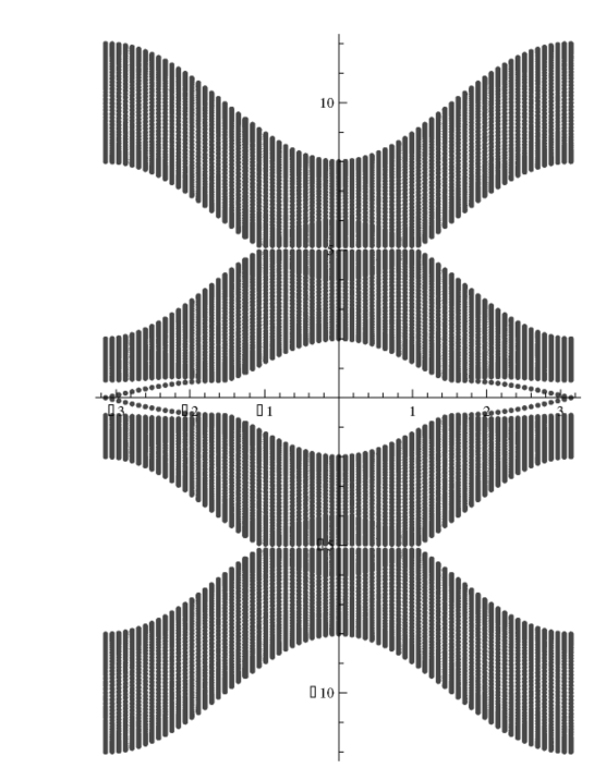
Figure 3: The energy spectra of 2D NCS with edges at $i_{x}=0$ and $i_{x}=50$ in the phases I, II, III and IV in Fig.1 a). Here $k_{y}$ denotes the momentum in the $y$-direction. We take $t=1$, $\mu=-3$, $\alpha=0.6$, $\Delta_{\rm t}=0.6$ and $\Delta_{\rm s}=0.1$. $H_{z}$ is I) $\mu_{\rm B}H_{z}=0$, II) $\mu_{\rm B}H_{z}=1.5$, III) $\mu_{\rm B}H_{z}=5$, and IV) $\mu_{\rm B}H_{z}=8$.

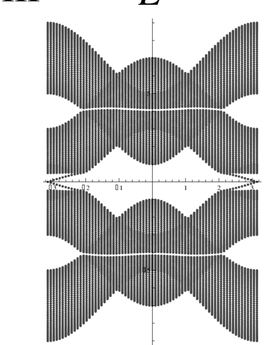
Figure 4: The energy spectra of 2D NCS with edges at $i_{x}=0$ and $i_{x}=50$ in phases I’ II’ III’ and IV’ in Fig.1 b). Here $k_{y}$ denotes the momentum in the $y$-direction. We take $t=1$, $\mu=-1$, $\alpha=0.6$, $\Delta_{\rm t}=0.6$ and $\Delta_{\rm s}=0.1$. $H_{z}$ is I’) $\mu_{\rm B}H_{z}=0$, II’) $\mu_{\rm B}H_{z}=1$, III’) $\mu_{\rm B}H_{z}=3$, IV’) $\mu_{\rm B}H_{z}=5$.

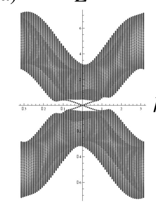
Figure 5: The dependence of gapless edge states in the phase I on the direction of the magnetic field. We take $t=1$, $\mu=-3$, $\alpha=0.6$, $\Delta_{\rm t}=0.6$ and $\Delta_{\rm s}=0,1$ a) $\mu_{\rm B}H_{x}=0.15$, $\mu_{\rm B}H_{y}=0$ and $\mu_{\rm B}H_{z}=0$. b) $\mu_{\rm B}H_{x}=0$, $\mu_{\rm B}H_{y}=0.15$ and $\mu_{\rm B}H_{z}=0$. A similar dependence is obtained for gapless edge states in the phase I’.

III.3 Transport phenomena associated with edge states

The existence of gapless edge states revealed by the previous subsections implies that transport phenomena associated with the edge states are possible in analogy with the quantum Hall state and the ${\bm{Z}}_{2}$ topological insulator. Here, we discuss such phenomena in NCS. Transport properties inherent in edge states can be probed experimentally by using the Hall bar geometry considered before for the detection of edge states of the quantum (spin) Hall effect depicted in Fig. 6 McEuen et al. (1990); Wang and Goldman (1991); Bernevig et al. (2006). Since our systems are superconductors, it is important for the experimental detection to discriminate between contributions from supercurrents and currents carried by edge states. A simple approach suitable for this purpose is to use thermal transport measurements. To suppress contributions from the Bogoliubov quasiparticles in the bulk, we assume that temperature is sufficiently lower than the superconducting gap, $T\ll\Delta$, and also the superconducting gap does not have nodes where the gap vanishes. The thermal conductance for heat currents is defined by $G^{T}=I^{T}_{14}/(\Delta T)_{14}$ where $I^{T}_{ij}$ is a thermal current between contacts $i$ and $j$ in Fig. 6, and $(\Delta T)_{ij}$ is the temperature difference between these contacts. In contrast to the conductance for electric currents, the thermal conductance is not quantized but depends on temperature $T$. The $T$-dependence of $G^{T}$ governed by edge states obeys a power law $\propto T$, which can be distinguished from contributions from the bulk quasiparticles which decay like $\sim\exp(-\Delta/T)$. Furthermore, as discussed in Bernevig et al. (2006) in the case of the quantum spin Hall effect, in a six terminal measurement, there is no temperature difference between contacts 2 and 3 (or 5 and 6), because the edge current is dissipationless.

A direct probe of spin Hall current carried by edge states may be also possible by measuring magnetization due to spin accumulation at contacts as discussed for the spin Hall effect Murakami et al. (2004). Bulk supercurrents carried by Cooper pairs do not contribute to spin Hall currents even for a spin-triplet pairing state, and hence the spin Hall current between contacts 3 and 5 induced by a longitudinal voltage or temperature difference between contacts 1 and 4 is governed by edge states.

A more remarkable effect due to edge states is the existence of the non-local transport McEuen et al. (1990); Wang and Goldman (1991). The non-local conductance is given by a heat current between contacts 3 and 5 divided by the temperature difference between 2 and 6 in Fig.6, $G^{T}_{\rm NL}=I^{T}_{35}/(\Delta T)_{26}$. If contacts 3 and 5 are well separated from 2 and 6, the nonzero $G^{T}_{NL}$ can not be explained by the bulk quasiparticles, which provides a direct evidence for the existence of current-carrying edge states.

In the case with a sufficiently weak magnetic field, the spin Hall effect still exists as long as the direction of the magnetic field is perpendicular to the propagating direction of the edge states, because of the accidental symmetry of the Rashba model as discussed in Secs. II.3 and III.2. If the magnetic field is tilted, and the field component along the propagating direction is nonzero, a gap opens in the energy spectrum of the edge states; this leads to the suppression of the spin Hall current which can be observed as a drop in the temperature difference between contacts.

The gapless edge states are also observed experimentally as a zero bias peak of tunneling current Iniotakis et al. (2007). Our results suggest that structures of the zero bias peak is very sensitive to the direction of the magnetic field. Under a magnetic field perpendicular to the edge direction, the zero bias peak is observed, but under a magnetic field along the edge, a splitting of the conduction peak is observed due to a tiny gap of the gapless edge states.

The transport properties considered above are experimentally observable for 2D Rashba NCS with $\Delta_{\rm t}>\Delta_{\rm s}$ which do not possess gap-nodes.

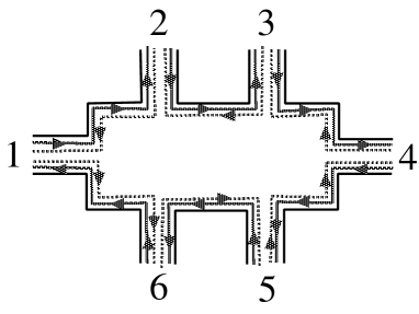
Figure 6: Hall bar with six terminals used for the detection of edge states. Solid and dotted gray lines with arrows represents propagating edge modes with different spin chirality corresponding to two SO split bands. These modes propagate in opposite directions.

IV Majorana zero energy modes in vortex cores and the non-Abelian statistics

In this section, we explore zero energy states in vortex cores for 2D NCS on the basis of both numerical and analytical approaches. We study the case with purely $p$-wave paring and the case with the admixture of $s$-wave and $p$-wave parings, respectively. It is assumed that no node exists in the superconducting gap because the existence of a full energy gap in the bulk is crucial for the stability of topological phases. As mentioned in the previous sections, as long as the gap of $p$-wave pairing is larger than that of $s$-wave pairing, the state is topologically equivalent to the purely $p$-wave pairing state, exhibiting topological nontriviality. In the following, we confirm this topological argument by obtaining explicitly the zero energy solutions of vortex cores. The condition for the non-Abelian statistics of vortices is also clarified on the basis of the explicit solutions.

IV.1 Numerical analysis of BdG equations

In this subsection, we analyze the low energy states in a vortex core of NCS by using numerical methods. For this purpose, we consider the following two dimensional tight-binding model for a Rashba superconductor with the admixture of $s$-wave and $p$-wave pairings,

$$\mathcal{H} = -t\sum_{\langle{\bm{i}},{\bm{j}}\rangle,\sigma}c^{\dagger}_{{\bm{i}}\sigma}c_{{\bm{j}}\sigma}-\mu\sum_{{\bm{i}},\sigma}c^{\dagger}_{{\bm{i}}\sigma}c_{{\bm{i}}\sigma}-\mu_{\rm B}H_{z}\sum_{{\bm{i}},\sigma,\sigma^{\prime}}(\sigma_{z})_{\sigma\sigma^{\prime}}c_{{\bm{i}}\sigma}^{\dagger}c_{{\bm{i}}\sigma^{\prime}}-i\frac{\alpha}{2}\sum_{\langle{\bm{i}},{\bm{j}}\rangle,\sigma,\sigma^{\prime}}({\bm{\sigma}}_{\sigma\sigma^{\prime}}\times\hat{{\bm{r}}}_{{\bm{i}}{\bm{j}}})_{z}c^{\dagger}_{{\bm{i}}\sigma}c_{{\bm{j}}\sigma^{\prime}}$$ (31)

$$+\Delta_{\rm s}\sum_{\bm{i}}(e^{i\phi_{\bm{i}}}c^{\dagger}_{{\bm{i}}\uparrow}c^{\dagger}_{{\bm{i}}\downarrow}+{\rm h.c.})$$

$$-\frac{1}{2}\Delta_{\rm t}\sum_{\bm{i}}(e^{i\phi_{{\bm{i}}+\frac{\hat{x}}{2}}}c^{\dagger}_{{\bm{i}}\uparrow}c^{\dagger}_{{\bm{i}}+\hat{x}\uparrow}-ie^{i\phi_{{\bm{i}}+\frac{\hat{y}}{2}}}c^{\dagger}_{{\bm{i}}\uparrow}c^{\dagger}_{{\bm{i}}+\hat{y}\uparrow}+e^{i\phi_{{\bm{i}}+\frac{\hat{x}}{2}}}c^{\dagger}_{{\bm{i}}\downarrow}c^{\dagger}_{{\bm{i}}+\hat{x}\downarrow}+ie^{i\phi_{{\bm{i}}+\frac{\hat{y}}{2}}}c^{\dagger}_{{\bm{i}}\downarrow}c^{\dagger}_{{\bm{i}}+\hat{y}\downarrow}+{\rm h.c.}).$$

Here the second and third lines of the right-hand side are, respectively, the $s$-wave and $p$-wave pairing terms, and a vortex located on the center of the system is incorporated into the phase $\phi_{\bm{i}}$ of the gap functions. To obtain the vortex core states for $\mathcal{H}$, we introduce the Bogoliubov quasiparticle operator,

$$\gamma^{\dagger}=\sum_{\bm{i}}[u_{\uparrow}({\bm{i}})c^{\dagger}_{{\bm{i}}\uparrow}+u_{\downarrow}({\bm{i}})c^{\dagger}_{{\bm{i}}\downarrow}+v_{\uparrow}({\bm{i}})c_{{\bm{i}}\uparrow}+v_{\downarrow}({\bm{i}})c_{{\bm{i}}\downarrow}].$$ (32)

The Bogoliubov-de Gennes (BdG) equations is derived from the relation $[\mathcal{H},\gamma^{\dagger}]=E\gamma^{\dagger}$. We solve the BdG equations numerically, and calculate the density profile of quasiparticles for low energy states.

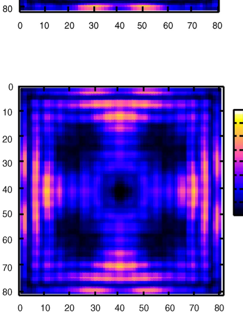
Figure 7: The density of quasiparticles for the purely $p$ wave state plotted on the $81\times 81$ $xy$-plane for some low energies $E$. The top and bottom panels are, respectively, the plots of $|u_{\uparrow}({\bm{r}})|^{2}+|u_{\downarrow}({\bm{r}})|^{2}$ and $|v_{\uparrow}({\bm{r}})|^{2}+|v_{\downarrow}({\bm{r}})|^{2}$ for $\alpha=t$, $\Delta_{\rm t}=0.05t$, $\mu_{\rm B}H_{z}=0$, $\mu=-3.75t$. $E=4.87\times 10^{-4}t$ (left), $E=7.67\times 10^{-4}t$ (middle), $E=1.023\times 10^{-3}t$ (right). For $E=4.87\times 10^{-4}t$ and $E=1.023\times 10^{-3}t$, edge states appear.

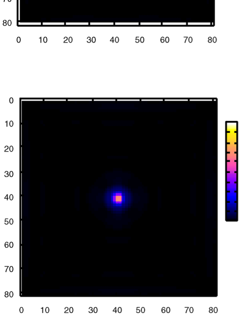
Figure 8: The density of quasiparticles for the purely $p$ wave state plotted on the $81\times 81$ $xy$-plane for low energies. The top and bottom panels are, respectively, the plots of $|u_{\uparrow}({\bm{r}})|^{2}+|u_{\downarrow}({\bm{r}})|^{2}$ and $|v_{\uparrow}({\bm{r}})|^{2}+|v_{\downarrow}({\bm{r}})|^{2}$. $\alpha=t$, $\Delta_{\rm t}=0.05t$, $\mu_{\rm B}H_{z}=0.04t$, $\mu=-4.0t$. $E=0.00123t$ (left), $E=0.0182t$ (middle), $E=0.0315t$ (right). Edge states appear for $E=0.0182t$ and $E=0.0315t$.

We, first, consider the case with a purely $p$-wave pairing. In Fig.7, the density of quasiparticles plotted on the $xy$-plane is shown. There are low energy vortex core states. The lowest energy for the vortex core state is $E=0.000767t$. For our choice of parameters in this calculation, $\Delta_{\rm t}^{2}/E_{F}\sim 0.005$. Thus, the vortex core state has much smaller energy than that of the conventional Caroli-de Gennes-Matricon mode. Furthermore, we find edge states with low energies as shown in Fig.7. The existence of low energy edge states is a concomitant of zero energy modes in vortex cores, and characterizes topological nature of the state. Therefore, we conclude that the zero energy vortex core states exist.

The zero energy vortex core states and the low energy edge states survive even when a Zeeman field along the $z$-direction is applied. The calculated results in this case is shown in Fig.8.

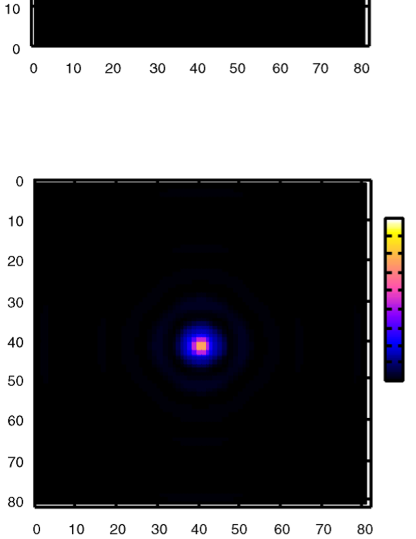
Figure 9: The density of quasiparticles for the $s+p$ wave state plotted on the $81\times 81$ $xy$-plane for low energies. The top and bottom panels are, respectively, the plots of $|u_{\uparrow}({\bm{r}})|^{2}+|u_{\downarrow}({\bm{r}})|^{2}$ and $|v_{\uparrow}({\bm{r}})|^{2}+|v_{\downarrow}({\bm{r}})|^{2}$. $\alpha=t$, $\Delta_{\rm t}=0.05t$, $\Delta_{\rm s}=-0.02t$, $\mu_{\rm B}H_{z}=0$, $\mu=-4.0t$. $E=0.0023t$ (left), $E=0.039t$ (middle), $E=0.0434t$ (right). Edge states appear for $E=0.0434t$.

We, next, consider the case with the admixture of $s$-wave pairing and $p$-wave pairing. The numerical results shown in Fig.9 demonstrate that the topological phase with gapless edge modes and zero energy vortex core states is stable as long as the gap of $p$-wave pairing is larger than that of $s$-wave pairing. As the magnitude of $|\Delta_{\rm s}|$ approaches $|\Delta_{\rm t}|$, the gap in one of two SO split bands $|\Delta_{\rm t}|-|\Delta_{\rm s}|$ decreases, and the spectrum gap in the vortex core becomes smaller, which makes it difficult to clarify the existence of zero energy vortex core states numerically. The numerical approach in this section is applicable only when $|\Delta_{\rm t}|-|\Delta_{\rm s}|$ is not much smaller than $|\Delta_{\rm t}|$.

To discuss whether the non-Abelian statistics of vortices is possible or not, we need to examine the degeneracy of Majorana modes. The numerical analysis presented in this subsection is not suitable for this purpose because of the limitation of the system size used in the numerics. To attack this issue, we exploit an analytical method in Sec. IV.4.

IV.2 A comment on the use of the chirality basis for the issues of vortex core states

Here, we discuss the limitation of the use of the chirality basis for the issues of vortex core states. For concreteness, we consider a noncentrosymmetric $s$-wave superconductor. In the absence of Zeeman fields, in homogeneous bulk systems without vortices, the unitary transformation $(a_{{\bm{k}}+},a_{{\bm{k}}-})^{T}=\hat{U}({\bm{k}})(c_{{\bm{k}}\uparrow},c_{{\bm{k}}\downarrow})^{T}$ with

$$\hat{U}({\bm{k}})=\frac{1}{\sqrt{2}}\left(\begin{array}[]{cc}1&e^{-i\theta({\bm{k}})}\\ -e^{i\theta({\bm{k}})}&1\end{array}\right),$$ (35)

which diagonalizes the asymmetric SO interaction in the spin space transforms the $s$-wave pairing terms into the intra-band pairing terms in the chirality basis,

$$\sum_{\nu=\pm}\sum_{\bm{k}}\Delta_{\rm s}e^{\nu i\theta({\bm{k}})}a_{{\bm{k}}\nu}^{\dagger}a_{-{\bm{k}}\nu}^{\dagger}+{\rm h.c.},$$ (36)

where $e^{\pm i\theta({\bm{k}})}\equiv-(\mathcal{L}_{0x}\pm i\mathcal{L}_{0y})/\sqrt{\mathcal{L}_{0x}^{2}+\mathcal{L}_{0y}^{2}}$ is an odd-parity phase factor. The above expression is similar to the pairing term of $p+ip$ superconductors. Thus, one may expect that zero energy vortex core modes exist when vortices are introduced into the system. However, this is not true. The unitary transformation (35) is derived for spatially homogeneous systems, and generally its use is not allowed in the case with vortices. In the case that quasiclassical approximation is justified, and the center of mass coordinate of Cooper pairs which characterizes inhomogeneity of the system is approximately commutative with the momentum operator ${\bm{k}}$ and the unitary transformation $\hat{U}({\bm{k}})$, the chirality basis can be used for the description of the vortex state, as done in Hayashi et al. (2006); Nagai et al. (2006); Fujimoto (2007b). However, to examine whether the zero energy mode exists or not in a vortex core, one needs to go beyond the quasiclassical approximation; i.e. the unitary transformation for homogeneous systems (35) is not applicable to the issue that we are concerned with here. Missing this consideration in Fujimoto (2008) leads to an incorrect conclusion that zero energy vortex core states exist even for purely $s$-wave NCS. For the clarification of the existence of zero energy modes in vortex cores, a powerful and reliable approach is to exploit the method developed by Tewari, Sarma and Lee which is analogous to the Jackiw-Rebbi’s index theorem Tewari et al. (2007b); Jackiw and Rebbi (1976). We consider this issue in the subsequent sections.

IV.3 Majorana zero energy modes in vortex cores: Index theorem

In this subsection, we develop an analytical approach for zero energy vortex core states which is a generalization of the index theorem for $p+ip$ superconductors obtained in Tewari et al. (2007b) to the case of noncentrosymmetric systems. We consider the model for a Rashba superconductor in two dimensions with a vortex located on the center of the system. The Hamiltonian is

$$\mathcal{H}=\mathcal{H}_{\rm K}+\mathcal{H}_{\rm SO}+\mathcal{H}_{\rm Ps}+\mathcal{H}_{\rm Pt},$$

$$\mathcal{H}_{\rm K}=\sum_{{\bm{k}},\sigma}\xi_{{\bm{k}}\sigma}c^{\dagger}_{{\bm{k}}\sigma}c_{{\bm{k}}\sigma},$$

$$\mathcal{H}_{\rm SO}=\alpha\sum\mbox{\boldmath$\mathcal{L}$}({\bm{k}})\cdot{\bm{\sigma}}_{\sigma\sigma^{\prime}}c^{\dagger}_{{\bm{k}}\sigma}c_{{\bm{k}}\sigma^{\prime}},\quad\mbox{\boldmath$\mathcal{L}$}({\bm{k}})=(k_{y},-k_{x},0),$$

$$\mathcal{H}_{\rm Ps}=\Delta_{\rm s}\int d^{2}{\bm{R}}d^{2}{\bm{r}}e^{i\phi_{R}}h_{s}({\bm{R}})g_{s}({\bm{r}})c^{\dagger}_{{\bm{R}}+{\bm{r}}\uparrow}c^{\dagger}_{{\bm{R}}-{\bm{r}}\downarrow}+{\rm h.c.},$$

$$\mathcal{H}_{\rm Pt}=-\frac{1}{2}\Delta_{\rm t}\int d^{2}{\bm{R}}d^{2}{\bm{r}}e^{i\phi_{R}}h_{s}({\bm{R}})[g_{\uparrow}({\bm{r}})c^{\dagger}_{{\bm{R}}+{\bm{r}}\uparrow}c^{\dagger}_{{\bm{R}}-{\bm{r}}\uparrow}+g_{\downarrow}({\bm{r}})c^{\dagger}_{{\bm{R}}+{\bm{r}}\downarrow}c^{\dagger}_{{\bm{R}}-{\bm{r}}\downarrow}]+{\rm h.c.},$$ (37)

where the band dispersion in the case with the Zeeman field $H_{z}$ is $\xi_{{\bm{k}}\sigma}=\epsilon_{\bm{k}}-\mu-\sigma\mu_{\rm B}H_{z}$ with $\epsilon_{\bm{k}}={\bm{k}}^{2}/2m$ and $\mu$ a chemical potential. $\mathcal{H}_{\rm SO}$ is the Rashba SO interaction with the coupling constant $\alpha$. $\mathcal{H}_{\rm Ps}$ and $\mathcal{H}_{\rm Pt}$ are, respectively, the pairing interaction for spin-singlet and spin-triplet channels. The center of mass coordinate and the relative coordinate for Cooper pairs are, respectively, represented by ${\bm{R}}$ and ${\bm{r}}$. The phase $\phi_{R}$ is due to the vortex at ${\bm{R}}=0$. The suppression of the superconducting order parameter in the vicinity of the vortex is incorporated into the functions $h_{a}({\bm{R}})=1-e^{-|{\bm{R}}|/\xi_{a}}$ with $a={\rm s}$ for the spin-singlet pair and $a={\rm t}$ for the spin-triplet pair. $g_{\rm s}({\bm{r}})$, $g_{\uparrow}({\bm{r}})$, and $g_{\downarrow}({\bm{r}})$ are the structure functions corresponding to the pairing symmetry. For simplicity, in the following, we consider the case with $s$-wave pairing for the spin-singlet channel and the $p$-wave pairing for the spin-triplet channel. Then, the Fourier transforms for the gap structure functions are $g_{\rm s}({\bm{k}})=1$, $g_{\uparrow}({\bm{k}})=-i(k_{x}-ik_{y})$ and $g_{\downarrow}({\bm{k}})=-i(k_{x}+ik_{y})$. Here the form of the ${\bm{d}}$-vector for triplet pairs are determined so as to be consistent with the Rashba SO interaction. To discuss the zero energy state in the vortex core, we follow the approach developed in Tewari et al. (2007b), and use the angular momentum representation of the electron operators,

$$c_{{\bm{k}}\sigma}=\frac{1}{\sqrt{2\pi k}}\sum_{m=-\infty}^{\infty}c_{m,k\sigma}e^{im\phi_{k}},$$ (38)

where $k=|{\bm{k}}|$ and $\phi_{k}$ is the azimuthal angle of ${\bm{k}}$. $c_{m,k\sigma}$ satisfies the anticommutation relation $\{c_{m,k\sigma},c^{\dagger}_{n,p\sigma^{\prime}}\}=\delta_{mn}\delta_{\sigma\sigma^{\prime}}\delta(k-p)$. In this representation, the Hamiltonian is rewritten into the following form.

$$\mathcal{H}_{\rm K}=\sum_{m}\int\frac{dk}{(2\pi)^{2}}\xi_{k\sigma}c^{\dagger}_{m,k\sigma}c_{m,k\sigma},$$ (39)

$$\mathcal{H}_{\rm SO}=\alpha\sum_{m}\int\frac{dk}{(2\pi)^{2}}ik[c^{\dagger}_{m,k\uparrow}c_{m+1,k\downarrow}-c^{\dagger}_{m,k\downarrow}c_{m-1,k\uparrow}]$$ (40)

$$\mathcal{H}_{\rm Ps}=-i\Delta_{\rm s}\int dkdp\sum_{m}u_{m}(k,p)\sqrt{kp}[kc^{\dagger}_{1-m,k\uparrow}c^{\dagger}_{m,p\downarrow}+pc^{\dagger}_{-m,k\uparrow}c^{\dagger}_{m+1,p\downarrow}]+{\rm h.c.},$$ (41)

$$\mathcal{H}_{\rm Pt}=\Delta_{\rm t}\int dkdp\sum_{m}[\{u_{m}(k,p)k-u_{m+1}(k,p)p\}k\sqrt{kp}c^{\dagger}_{-m,k\uparrow}c^{\dagger}_{m,p\uparrow}+u_{m}(k,p)k^{2}\sqrt{kp}c^{\dagger}_{2-m,k\downarrow}c^{\dagger}_{m,p\downarrow}]+{\rm h.c.}.$$ (42)

Here $u_{m}(k,p)$ is the Fourier transform of $1/|{\bm{k}}+{\bm{p}}|^{3}$.

$$\frac{1}{|{\bm{k}}+{\bm{p}}|^{3}}=\sum_{m}u_{m}(k,p)e^{-im(\phi_{\bm{k}}-\phi_{\bm{p}})}.$$ (43)

In Eqs.(39),(40), (41) and (42), the $m=0$ mode with up spin and the $m=1$ mode with down spin are decoupled from other modes. The pairing interaction terms for these modes are

$$\mathcal{H}_{\rm Ps}^{(01)}=-i\Delta_{\rm s}\int dkdp\sqrt{kp}[u_{1}(k,p)k+u_{0}(k,p)p]c^{\dagger}_{0,k\uparrow}c^{\dagger}_{1,p\downarrow}+{\rm h.c.},$$

$$\mathcal{H}_{\rm Pt}^{(01)}=\Delta_{\rm t}\int dkdp[\{u_{0}(k,p)k-u_{1}(k,p)p\}k\sqrt{kp}c^{\dagger}_{0,k\uparrow}c^{\dagger}_{0,p\uparrow}+u_{1}(k,p)k^{2}\sqrt{kp}c^{\dagger}_{1,k\downarrow}c^{\dagger}_{1,p\downarrow}]+{\rm h.c.}.$$ (44)

In $\mathcal{H}_{\rm Pt}^{(01)}$, the term with $u_{1}(k,p)$ for the $\uparrow\uparrow$ pairs vanishes because of the symmetric property $u_{1}(k,p)=u_{1}(p,k)$. Thus, we have

$$\mathcal{H}^{(01)}_{\rm Pt}=\Delta_{t}\int dkdp\sqrt{kp}k^{2}[u_{0}(k,p)c^{\dagger}_{0,k\uparrow}c^{\dagger}_{0,p\uparrow}+u_{1}(k,p)c^{\dagger}_{1,k\downarrow}c^{\dagger}_{1,p\downarrow}]+{\rm h.c.}.$$ (45)

IV.3.1 Purely $p$-wave pairing

We, first, consider the purely triplet case, i.e. $\Delta_{\rm s}=0$. Then, the Hamiltonian for the $m=0$ mode with up spin and the $m=1$ mode with down spin is

$$\mathcal{H}^{(01)} = \int\frac{dk}{(2\pi)^{2}}[\xi_{k\uparrow}c^{\dagger}_{0,k\uparrow}c_{0,k\uparrow}+\xi_{k\downarrow}c^{\dagger}_{1,k\downarrow}c_{1,k\downarrow}]$$ (46)

$$+ i\alpha\int\frac{dk}{(2\pi)^{2}}k[c^{\dagger}_{0,k\uparrow}c_{1,k\downarrow}-c^{\dagger}_{1,k\downarrow}c_{0,k\uparrow}]$$

$$- \int dkdp[\tilde{\Delta}_{{\rm t}0}(k,p)c^{\dagger}_{0,k\uparrow}c^{\dagger}_{0,p\uparrow}-\tilde{\Delta}_{{\rm t}1}c^{\dagger}_{1,k\downarrow}c^{\dagger}_{1,p\downarrow}+{\rm h.c.}],$$

with $\tilde{\Delta}_{\rm t0}(k,p)=\Delta_{\rm t}\sqrt{kp}(k^{2}-p^{2})u_{0}(k,p)/2$, and $\tilde{\Delta}_{\rm t1}(k,p)=-\Delta_{\rm t}\sqrt{kp}(k^{2}-p^{2})u_{1}(k,p)/2$. Here we have antisymmetrized the spin-triplet pairing terms. In the Fourier coefficients,

$$u_{0}(k,p)=\int\frac{d(\phi_{\bm{k}}-\phi_{\bm{p}})}{2\pi}\frac{1}{|{\bm{k}}+{\bm{p}}|^{3}},$$ (47)

$$u_{1}(k,p)=\int\frac{d(\phi_{\bm{k}}-\phi_{\bm{p}})}{2\pi}\frac{e^{i(\phi_{\bm{k}}-\phi_{\bm{p}})}}{|{\bm{k}}+{\bm{p}}|^{3}},$$ (48)

the most dominant contributions are from $\phi_{\bm{k}}-\phi_{\bm{p}}\sim\pm\pi$, which implies $u_{1}(k,p)<0$ and $u_{0}(k,p)>0$. By using the unitary transformation

$$c_{0,k\uparrow}=\zeta_{+}(k)a_{k+}+i\zeta_{-}(k)a_{k-},$$ (49)

$$c_{1,k\downarrow}=i\zeta_{-}(k)a_{k+}+\zeta_{+}(k)a_{k-},$$ (50)

with

$$\zeta_{\pm}(k)=\sqrt{\frac{1}{2}\left(1\pm\frac{H_{z}}{\sqrt{\alpha^{2}k^{2}+H_{z}^{2}}}\right)},$$ (51)

we rewrite the Hamiltonian (46) as,

$$\mathcal{H}^{(01)} = \sum_{\nu=\pm}\bigl{[}\int\frac{dk}{(2\pi)^{2}}\xi_{k}^{(\nu)}a^{\dagger}_{k\nu}a_{k\nu}+\int dk\int dp\{\tilde{\Delta}_{\nu}(k,p)a^{\dagger}_{k\nu}a^{\dagger}_{p\nu}+{\rm h.c.}\}\bigr{]}$$ (52)

$$+ \int dk\int dp[\tilde{\Delta}_{2+}(k,p)a^{\dagger}_{k+}a^{\dagger}_{p-}+\tilde{\Delta}_{2-}(k,p)a^{\dagger}_{k-}a^{\dagger}_{p+}+{\rm h.c.}],$$

where

$$\tilde{\Delta}_{\pm}(k,p)=\pm\frac{\tilde{\Delta}_{\rm t0}+\tilde{\Delta}_{{\rm t}1}}{2}r_{+}(k,p)+\frac{\tilde{\Delta}_{\rm t0}-\tilde{\Delta}_{{\rm t}1}}{2}r_{-}(k,p),$$ (53)

$$\tilde{\Delta}_{2\pm}(k,p)=\mp i\frac{\tilde{\Delta}_{\rm t0}+\tilde{\Delta}_{{\rm t}1}}{2}s_{-}(k,p)-i\frac{\tilde{\Delta}_{\rm t0}-\tilde{\Delta}_{{\rm t}1}}{2}s_{+}(k,p),$$ (54)

with $r_{\pm}(k,p)=\zeta_{+}(k)\zeta_{+}(p)\pm\zeta_{-}(k)\zeta_{-}(p)$, $s_{\pm}(k,p)=\zeta_{+}(k)\zeta_{-}(p)\pm\zeta_{-}(k)\zeta_{+}(p)$, and $\xi_{k}^{(\nu)}=\epsilon_{k}-\mu-\nu\sqrt{\alpha^{2}k^{2}+(\mu_{\rm B}H_{z})^{2}}$. We concentrate on low energy excitations in the vicinity of the Fermi surface, and write $k$ and $p$ as $k=k_{F\pm}+q$ and $p=k_{F\pm}+q^{\prime}$ where $k_{F+}$ and $k_{F-}$ are, respectively, the Fermi momenta for the two SO split bands, and $|q|,|q^{\prime}|\ll k_{F\pm}$. In Eq.(54), the first term is of the order $O((q-q^{\prime})^{2})$, because $\tilde{\Delta}_{\rm t0,1}(k,p)$ and $s_{-}(k,p)$ are antisymmetric with respect to the exchange of $k$ and $p$. We can neglect this term compared to other terms up to $O(q-q^{\prime})$. Furthermore, from Eqs.(47) and (48), we see that $|\tilde{\Delta}_{\rm t0}-\tilde{\Delta}_{\rm t1}|/|\tilde{\Delta}_{\rm t0}+\tilde{\Delta}_{\rm t1}|\sim O(1/R_{\rm c}^{2})$ where $R_{\rm c}$ is the system size, and in the limit of $R_{\rm c}\rightarrow\infty$, the second term of (54) is negligible compared to the first term of (53). As a result, the inter-band pairing terms can be neglected, and the Hamiltonian (52) is decoupled into two parts corresponding, respectively, to contributions from the two SO split bands, $\nu=+$ and $-$. $\tilde{\Delta}_{\pm}(k,p)\equiv A_{\pm}(q-q^{\prime})$ must be odd in $q-q^{\prime}$, since, otherwise, the pairing term in Eq.(52) vanishes. Then, the Fourier transforms of $A_{\pm}(q-q^{\prime})$ denoted as $\mp im_{\pm}(x)$ are odd functions of $x$. Here $m_{\pm}(x)$ is real.

Linearizing the band dispersion $\xi_{k\nu}$ around the Fermi momentum, and expressing the operator for the Bogoliubov quasiparticle as,

$$\gamma^{\dagger}_{\nu}=\int dx[\eta_{1\nu}a^{\dagger}_{\nu}(x)+\eta_{2\nu}a_{\nu}(-x)],$$ (55)

we obtain the Bogoliubov-de-Gennes (BdG) equations from the relation $[\mathcal{H}^{(01)},\gamma^{\dagger}]=E\gamma^{\dagger}$,

$$-iv_{\nu}\sigma_{z}\partial_{x}\eta_{\nu}(x)+\nu m_{\nu}(x)\sigma_{y}\eta_{\nu}(x)=E\eta_{\nu}(x),$$ (56)

with $\nu=\pm$ corresponding to the two SO split bands and the Fermi velocities $v_{\nu}$. Here $\eta_{\pm}^{T}(x)=(\eta_{1\pm},\eta_{2\pm})$. The BdG equations have a zero energy solution with $E=0$ for each bands: When $m_{\pm}(x)$ satisfies $m_{\pm}(x)={\rm sgn}(x)|m_{\pm}(x)|$, the zero energy solutions are

$$\eta_{+}^{T}(x)=e^{-\frac{1}{v_{+}}\int^{x}_{0}m_{+}(y)dy}\frac{1}{\sqrt{2}}(1,1),$$ (57)

$$\eta_{-}^{T}(x)=e^{-\frac{1}{v_{+}}\int^{x}_{0}m_{-}(y)dy}\frac{i}{\sqrt{2}}(1,-1).$$ (58)

For these solutions (57) and (58), the quasiparticle operator (55) satisfies $\gamma_{\nu}^{\dagger}=\gamma_{\nu}$, and thus there are two Majorana fermion modes corresponding to the two bands.

It is noted that these two Majorana modes are stable against the magnetic field along $H_{z}$ in accordance with the existence of two gapless edge modes in this case as discussed in Sec. III.2. This phase is topologically equivalent to the phase I or I’ in Table 1.

IV.3.2 $s+p$ wave pairing

Now we consider the case with the admixture of the spin singlet pairs and spin triplet pairs. The Hamiltonian for the $m=0$ mode with up spin and the $m=1$ mode with down spin is

$$\mathcal{H}^{(01)} = \int\frac{dk}{(2\pi)^{2}}[\xi_{k\uparrow}c^{\dagger}_{0,k\uparrow}c_{0,k\uparrow}+\xi_{k\downarrow}c^{\dagger}_{1,k\downarrow}c_{1,k\downarrow}]$$ (59)

$$+ i\alpha\int\frac{dk}{(2\pi)^{2}}k[c^{\dagger}_{0,k\uparrow}c_{1,k\downarrow}-c^{\dagger}_{1,k\downarrow}c_{0,k\uparrow}]$$

$$- i\int dkdp\tilde{\Delta}_{\rm s}(k,p)[c^{\dagger}_{0,k\uparrow}c^{\dagger}_{1,p\downarrow}+{\rm h.c.}]$$

$$+ \int dkdp[\tilde{\Delta}_{\rm t0}(k,p)c^{\dagger}_{0,k\uparrow}c^{\dagger}_{0,p\uparrow}-\tilde{\Delta}_{\rm t1}(k,p)c^{\dagger}_{1,k\downarrow}c^{\dagger}_{1,p\downarrow}+{\rm h.c.}].$$

Here $\tilde{\Delta}_{\rm s}(k,p)=\Delta_{\rm s}\sqrt{kp}[u_{1}(k,p)k+u_{0}(k,p)p]$. The application of the unitary transformation (49) and (50) to the pairing terms of (59) gives,

$$\int dkdp[\tilde{\Delta}_{+}^{\prime}(k,p)a^{\dagger}_{k+}a^{\dagger}_{p+}+\tilde{\Delta}_{-}^{\prime}(k,p)a^{\dagger}_{k-}a^{\dagger}_{p-}+{\rm h.c.}]$$

$$-i\int dkdp[\tilde{i\Delta}_{2}^{\prime}(k,p)a^{\dagger}_{k+}a^{\dagger}_{p-}-i\tilde{\Delta}_{2}^{\prime}(p,k)a^{\dagger}_{k-}a^{\dagger}_{p+}+{\rm h.c.}],$$ (60)

where

$$\tilde{\Delta}_{\pm}^{\prime}(k,p)=\tilde{\Delta}_{\pm}(k,p)\mp\tilde{\Delta}_{\rm s}^{(s)}(k,p)s_{-}(k,p)-\tilde{\Delta}_{\rm s}^{(a)}(k,p)s_{+}(k,p),$$ (61)

$$\tilde{\Delta}_{2}^{\prime}(k,p)=\tilde{\Delta}_{\rm s}^{(s)}(k,p)r_{+}(k,p)+\tilde{\Delta}_{\rm s}^{(a)}(k,p)r_{-}(k,p),$$ (62)

with $\tilde{\Delta}_{\rm s}^{(s)}(k,p)=(\tilde{\Delta}_{\rm s}(k,p)+\tilde{\Delta}_{\rm s}(p,k))/4$ and $\tilde{\Delta}_{\rm s}^{(a)}(k,p)=(\tilde{\Delta}_{\rm s}(k,p)-\tilde{\Delta}_{\rm s}(p,k))/4$. It is reasonable to postulate that in the $s$-wave gap $\tilde{\Delta}_{\rm s}$, the symmetric part $\tilde{\Delta}_{\rm s}^{(s)}$ dominates, and $\tilde{\Delta}_{\rm s}^{(a)}$ can be neglected. We write $k=k_{F\pm}+q$, $p=k_{F\pm}+q^{\prime}$ with $q,q^{\prime}\ll k_{F\pm}$ as before. $\tilde{\Delta}_{\pm}^{\prime}(k,p)\equiv\pm A_{\rm t}(q-q^{\prime})$ is odd in $q-q^{\prime}$, while $\tilde{\Delta}_{2}^{\prime}(k,p)\equiv A_{\rm s}(q-q^{\prime})$ is even in $q-q^{\prime}$. Fourier transforming to the coordinate space, we introduce the quasiparticle operator,

$$\gamma^{\dagger}=\int dx[\eta_{1+}(x)a^{\dagger}_{+}(x)+\eta_{2+}(x)a_{+}(-x)+\eta_{1-}(x)a^{\dagger}_{-}(x)+\eta_{2-}(x)a_{-}(-x)].$$ (63)

The Fourier transform of the odd-parity pairing term is

$$\nu\int dx~{}im_{\rm t}(x)a^{\dagger}_{\nu}(x)a^{\dagger}_{\nu}(-x)+{\rm h.c.},\qquad\nu=\pm,$$ (64)

while for the even-parity pairing term,

$$i\int dx~{}m_{\rm s}(x)a^{\dagger}_{+}(x)a^{\dagger}_{-}(-x)+{\rm h.c.}.$$ (65)

Here, $m_{\rm t}(x)$ ($m_{\rm s}(x)$) is the Fourier transform of $A_{\rm t}(q)$ ($A_{\rm s}(q)$) and odd (even) in $x$. Then, the BdG equations for $\Psi^{T}(x)=(\eta_{1+}(x),\eta_{2+}(x),\eta_{1-}(x),\eta_{2-}(x))$ are,

$$-iv\partial_{x}\eta_{1+}(x)-im_{\rm t}(x)\eta_{2+}(x)-im_{\rm s}(x)\eta_{2-}(x)=E\eta_{1+}(x),$$

$$iv\partial_{x}\eta_{2+}(x)+im_{\rm t}(x)\eta_{1+}(x)-im_{\rm s}(x)\eta_{1-}(x)=E\eta_{2+}(x),$$

$$-iv\partial_{x}\eta_{1-}(x)+im_{\rm t}(x)\eta_{2-}(x)+im_{\rm s}(x)\eta_{2+}(x)=E\eta_{1-}(x),$$

$$iv\partial_{x}\eta_{2-}(x)-im_{\rm t}(x)\eta_{1-}(x)+im_{\rm s}(x)\eta_{1+}(x)=E\eta_{2-}(x).$$ (66)

Here, to simplify the analysis, we have assumed $v_{+}\approx v_{-}\equiv v$ which is justified for $E_{F}\gg\alpha$. From Eq. (66), we find two sets of solutions with zero energy eigen value $E=0$ up to normalization factors,

$$\Psi_{1}^{T}(x)=(C_{+}(x),C_{+}(x),-C_{-}(x),C_{-}(x)),$$ (67)

$$\Psi_{2}^{T}(x)=(-iC_{-}(x),-iC_{-}(x),iC_{+}(x),-iC_{+}(x)),$$ (68)

with

$$C_{\pm}(x)=e^{-\frac{1}{v}\int^{x}_{x_{+}}dy[m_{\rm t}(y)+m_{\rm s}(y)]}\pm e^{-\frac{1}{v}\int^{x}_{x_{-}}dy[m_{\rm t}(y)-m_{\rm s}(y)]},$$ (69)

and $x_{\pm}$ the solution of $m_{t}(x_{\pm})\pm m_{s}(x_{\pm})=0$. We can easily verify that $x_{-}=-x_{+}$ and $C_{+}(x)$ ($C_{-}(x)$) is an even (odd) function of $x$. The above solutions (67) and (68) are normalizable only when $m_{\rm t}(x)\pm m_{\rm s}(x)>0$ for $x>x_{\pm}$ and $m_{\rm t}(x)\pm m_{\rm s}(x)<0$ for $x<x_{\pm}$. Therefore as long as the gap for the spin-triplet pairs is larger than that for the spin-singlet pairs, the zero energy modes exist, which is consistent with the recent result obtained by Lu and Yip Lu and Yip . It is noted that the quasiparticle operator (63) for the solutions (67) and (68) satisfies $\gamma^{\dagger}=\gamma$; the quasiparticles corresponding to these solutions are Majorana fermions.

The phase with the two Majorana fermion modes is classified as the phase I or I’ in Table 1.

IV.4 Non-Abelian statistics of vortices

The non-Abelian statistics of vortices is realized when there is only one Majorana mode in a vortex core Read and Green (2000); Ivanov (2001); Sato (2003). Thus, it is necessary to eliminate one of two Majorana fermion modes found in Sec. IV.3. For this purpose, we consider the case that the Fermi level crosses the $\Gamma$ point in the Brillouin zone; i.e. $\varepsilon_{{\bm{k}}={\bm{0}}}-\mu=0$ ($\mu=-4t$). Then, for $H_{z}\neq 0$, a gap $\sim\mu_{\rm B}H_{z}$ opens in the vicinity of the $\Gamma$ point at the Fermi level Fujimoto (2008).

In the case of purely $p$-wave pairing, this implies that $v_{-}$ in (56) vanishes, and instead the mass term $2\sigma_{z}|\mu_{\rm B}H_{z}|\eta_{-}(x)$ is added. In this case, there is no zero energy mode for the $\nu=-$ band, and there is only one zero energy Majorana mode for the quasiparticles with the Fermi momentum $k_{F+}$($\neq 0$) in the $\nu=+$ band, which ensures the non-Abelian statistics of vortices Fujimoto (2008). This state is topologically equivalent to the phase II in Table 1, and also to spinless $p+ip$ superconductivity. However, the realization of this state in NCS is more feasible than that of spinless $p+ip$ superconductivity, because, for spinless $p+ip$ state, the strong magnetic field associated with full spin polarization leads to the fatal orbital depairing effect on superconductivity, while, for the Rashba NCS with $\mu=-4t$, a weak magnetic field between $H_{\rm c1}$ and $H_{\rm c2}$ applied parallel to the $z$-axis is sufficient to eliminate one of two Majorana modes.

In a similar manner, in the case of $s+p$-wave pairing with $|\Delta_{\rm t}|>|\Delta_{\rm s}|$, for $\mu=-4t$, there remains only one zero energy mode: The BdG equations for the quasiparticle operator (63) with $E=0$ becomes

$$-iv\partial_{x}\eta_{1+}(x)-im_{\rm t}(x)\eta_{2+}(x)-im_{\rm s}(x)\eta_{2-}(x)=0,$$

$$iv\partial_{x}\eta_{2+}(x)+im_{\rm t}(x)\eta_{1+}(x)-im_{\rm s}(x)\eta_{1-}(x)=0,$$

$$|2\mu_{\rm B}H_{z}|\eta_{1-}(x)+im_{\rm t}(x)\eta_{2-}(x)+im_{\rm s}(x)\eta_{2+}(x)=0,$$

$$-|2\mu_{\rm B}H_{z}|\eta_{2-}(x)-im_{\rm t}(x)\eta_{1-}(x)+im_{\rm s}(x)\eta_{1+}(x)=0.$$ (70)

When $m_{\rm t}(x)$ satisfies $m_{\rm t}(x)={\rm sgn}(x)|m_{\rm t}(x)|$, (70) has only one normalizable solution,

$$\eta_{1+}(x)=C(x),\quad\eta_{2+}=C(x),\quad\eta_{1-}(x)=\frac{m_{\rm s}(x)(m_{\rm t}(x)-2i|\mu_{\rm B}H_{z}|)}{4(\mu_{\rm B}H_{z})^{2}+m_{\rm t}^{2}(x)},\quad\eta_{2-}(x)=-\frac{m_{\rm s}(x)(m_{\rm t}(x)-2i|\mu_{\rm B}H_{z}|)}{4(\mu_{\rm B}H_{z})^{2}+m_{\rm t}^{2}(x)},$$ (71)

with

$$C(x)=e^{-\frac{1}{v}\int_{0}^{x}\frac{m_{\rm t}(y)(4(\mu_{\rm B}H_{z})^{2}+m_{\rm t}^{2}(y)-m_{\rm s}^{2}(y))-2im_{\rm s}^{2}(y)|\mu_{\rm B}H_{z}|}{4(\mu_{\rm B}H_{z})^{2}+m_{\rm t}(y)}dy}.$$ (72)

For this solution, the quasiparticle operator is

$$\gamma^{\dagger}=\int dxC(x)\left[a_{+}^{\dagger}(x)+a_{+}(-x)+\frac{m_{\rm s}(x)(m_{\rm t}(x)-2i|\mu_{\rm B}H_{z}|)}{4(\mu_{\rm B}H_{z})^{2}+m_{\rm t}^{2}(x)}(a_{-}^{\dagger}(x)-a_{-}(-x))\right],$$ (73)

which satisfies $\gamma^{\dagger}=\gamma$. Thus, there is only one Majorana zero energy mode in a vortex core. Under this situation, the non-Abelian statistics of vortices is possible.

IV.5 Majorana condition

The Majorana condition of zero energy vortex core states is crucial to the non-Abelian statistics of the vortices, so it is better to argue it without any approximation. In this section, we present a general argument on the Majorana condition of vortex zero modes for the 2D NCS.

Let us start with (59) in the Nambu representation,

$${\cal H}^{(01)}=\frac{1}{2}\int\frac{dkdp}{(2\pi)^{2}}\left(c_{0,k\uparrow}^{\dagger},c_{1,k\downarrow}^{\dagger},c_{0,k\uparrow},c_{1,k\downarrow}\right){\cal H}(k,p)\left(\begin{array}[]{c}c_{0,p\uparrow}\\ c_{1,p\downarrow}\\ c_{0,p\uparrow}^{\dagger}\\ c_{1,p\downarrow}^{\dagger}\end{array}\right),$$ (78)

where ${\cal H}(k,p)$ is given by

$${\cal H}(k,p)=\left(\begin{array}[]{cccc}\xi_{k\uparrow}\delta_{k,p}&i\alpha k\delta_{k,p}&h^{01}_{{\rm t}\uparrow}(k,p)&h^{01}_{\rm s}(k,p)\\ -i\alpha k\delta_{k,p}&\xi_{k\downarrow}\delta_{k,p}&-h^{01}_{\rm s}(p,k)&h^{01}_{{\rm t}\downarrow}(k,p)\\ h^{01*}_{{\rm t}\uparrow}(p,k)&-h^{01*}_{\rm s}(k,p)&-\xi_{k\uparrow}\delta_{k,p}&i\alpha k\delta_{k,p}\\ h^{01*}_{\rm s}(p,k)&h^{01*}_{{\rm t}\downarrow}(p,k)&-i\alpha k\delta_{k,p}&-\xi_{k\downarrow}\delta_{k,p}\end{array}\right)$$ (83)

with

$$h^{01}_{\rm s}(k,p)=-i(2\pi)^{2}\tilde{\Delta}_{\rm s}(k,p),\quad h^{01}_{{\rm t}\uparrow}(k,p)=2(2\pi)^{2}\tilde{\Delta}_{\rm t0}(k,p)\quad h^{01}_{{\rm t}\downarrow}(k,p)=-2(2\pi)^{2}\tilde{\Delta}_{\rm t1}(k,p).$$

Using the following relation,

$$\left(\begin{array}[]{c}c_{0,p\uparrow}\\ c_{1,p\downarrow}\\ c_{0,p\uparrow}^{\dagger}\\ c_{1,p\downarrow}^{\dagger}\end{array}\right)=\Gamma\left(\begin{array}[]{c}c_{0,p\uparrow}\\ c_{1,p\downarrow}\\ c_{0,p\uparrow}^{\dagger}\\ c_{1,p\downarrow}^{\dagger}\end{array}\right)^{*},\quad\Gamma=\left(\begin{array}[]{cc}0&{\bm{1}}_{2\times 2}\\ {\bm{1}}_{2\times 2}&0\end{array}\right),$$ (95)

one can show that ${\cal H}(k,p)$ has the so-called particle hole symmetry,

$$\Gamma{\cal H}(k,p)\Gamma=-{\cal H}^{*}(k,p),$$ (96)

which also can be checked directly from (83).

In the momentum space, the BdG equation is given by,

$$\int dp{\cal H}(k,p){\bm{u}}(p)=E{\bm{u}}(k),$$ (97)

where ${\bm{u}}(p)$ is a four component vector ${\bm{u}}(p)=(\alpha(p),\beta(p),\gamma(p),\delta(p))^{\rm t}$. When ${\bm{u}}(p)$ is a solution of the BdG equation with the energy $E$, then, using (96), we can show that $\Gamma{\bm{u}}^{*}(p)$ is a solution with the energy $-E$,

$$\int dp{\cal H}(k,p)\Gamma{\bm{u}}^{*}(p)=-E\Gamma{\bm{u}}^{*}(k).$$ (98)

Therefore, if ${\bm{u}}_{0}(p)$ is a zero mode of the BdG equation, then $\Gamma{\bm{u}}_{0}^{*}(p)$ is also a zero mode. This means that if the BdG equation has only one independent zero mode ${\bm{u}}_{0}(p)$, then ${\bm{u}}_{0}(p)$ and $\Gamma{\bm{u}}_{0}(p)$ should not be independent of each other. In general, if there are an odd number of independent zero modes, then at least for one solution, ${\bm{u}}_{0}(p)$ and $\Gamma{\bm{u}}_{0}^{*}(p)$ are not independent.

For simplicity, suppose that the BdG equation has a single zero mode ${\bm{u}}_{0}(p)$. As mentioned above, ${\bm{u}}_{0}(p)$ and $\Gamma{\bm{u}}_{0}^{*}(p)$ are not independent, so we have

$${\bm{u}}_{0}(p)=\Gamma{\bm{u}}_{0}^{*}(p),$$ (99)

by choosing a suitable phase of ${\bm{u}}_{0}(p)$. In terms of the components of ${\bm{u}}_{0}(p)$, this becomes

$${\bm{u}}_{0}(p)\equiv\left(\begin{array}[]{c}\alpha_{0}(p)\\ \beta_{0}(p)\\ \chi_{0}(p)\\ \eta_{0}(p)\end{array}\right)=\left(\begin{array}[]{c}\chi_{0}^{*}(p)\\ \eta_{0}^{*}(p)\\ \alpha_{0}^{*}(p)\\ \beta_{0}^{*}(p)\end{array}\right).$$ (108)

To obtain the annihilation operator $\gamma$ for the zero mode, we perform the mode expansion for $(c_{0p\uparrow},c_{1p\downarrow},c_{0p\uparrow}^{\dagger},c_{1p\downarrow}^{\dagger})$,

$$\left(\begin{array}[]{c}c_{0,p\uparrow}\\ c_{1,p\downarrow}\\ c_{0,p\uparrow}^{\dagger}\\ c_{1,p\downarrow}^{\dagger}\end{array}\right)=\gamma\left(\begin{array}[]{c}\alpha_{0}(p)\\ \beta_{0}(p)\\ \chi_{0}(p)\\ \eta_{0}(p)\end{array}\right)+\cdots,$$ (117)

where we have omitted the terms including non-zero modes. In this equation, we have two dependent relations,

$$c_{0,p\uparrow}=\gamma\alpha_{0}(p)+\cdots,\quad c_{0,p\uparrow}^{\dagger}=\gamma\chi_{0}(p)+\cdots,$$

$$c_{1,p\downarrow}=\gamma\beta_{0}(p)+\cdots,\quad c_{1,p\downarrow}^{\dagger}=\gamma\eta_{0}(p)+\cdots.$$ (118)

Thus $\gamma$ must satisfy the Majorana condition,

$$\gamma=\gamma^{\dagger}.$$ (119)

From the normalization condition for the zero mode, $\gamma$ can be written as

$$\gamma=\int dp(\alpha_{0}^{*}(p),\beta_{0}^{*}(p),\chi_{0}^{*}(p),\eta_{0}^{*}(p))\left(\begin{array}[]{c}c_{0,p\uparrow}\\ c_{1,p\downarrow}\\ c_{0,p\uparrow}^{\dagger}\\ c_{1,p\downarrow}^{\dagger}\end{array}\right).$$ (124)

Thus the commutation relation of $\eta_{0}$ can be calculated as

$$\{\gamma,\gamma^{\dagger}\} = \int dkdp\{\alpha_{0}^{*}(k)c_{0,k\uparrow}+\beta_{0}^{*}(k)c_{1,k\downarrow}+\chi_{0}^{*}(k)c_{0,k\uparrow}^{\dagger}+\eta_{0}^{*}(k)c_{1,k\downarrow}^{\dagger},$$ (125)

$$\hskip 21.52771pt\alpha_{0}(p)c_{0,p\uparrow}^{\dagger}+\beta_{0}(p)c_{1,p\downarrow}^{\dagger}+\chi_{0}(p)c_{0,p\uparrow}+\eta_{0}(p)c_{1,p\downarrow}\}$$

$$= \int dkdp\left[\alpha_{0}^{*}(k)\alpha_{0}(p)+\beta_{0}^{*}(k)\beta_{0}(p)+\chi_{0}^{*}(k)\chi_{0}(p)+\eta_{0}^{*}(k)\eta_{0}(p)\right]\delta_{k,p}$$

$$= 1$$

In a similar manner, we can show that $\gamma$ anti-commutes with annihilation and creation operators for non-zero modes.

In conclusion, the existence of only one zero energy mode in a vortex core is the necessary and sufficient condition for the existence of a single Majorana mode which leads to the non-Abelian statistics.

V Summary

We have explored topological phases of NCS characterized by the existence of gapless edge states and Majorana fermion modes in vortex cores, mainly focusing on the 2D Rashba superconductors with the admixture of $s$-wave pairing and $p$-wave pairing. It has been clarified that when the $p$-wave gap is larger than the $s$-wave gap, topological states are realized. We have completed the topological classification of these states by examining the TKNN number, the ${\bm{Z}}_{2}$ index, and the winding number associated with specific symmetry points in the Brillouin zone. It has been also found that for the Rashba superconductors, the gapless edge states that ensure the quantum spin Hall effect protected from disorder are stable against a weak magnetic field applied perpendicular to the propagating direction of the edge states, despite broken time-reversal symmetry which flaws the ${\bm{Z}}_{2}$ characterization of the topological phase. The stability of the edge states is guaranteed by a specific accidental symmetry of the Rashba model. We have also proposed a simple scheme for the realization of the non-Abelian statistics of vortices in topological phases of NCS under an applied magnetic field.

Experimental verification of these findings are particularly of interest. The topologically-protected gapless edge states play important roles for transport properties. In the superconducting state, current flows carried by the edge states can be detected by the measurement of a spin Hall current or thermal transport measurements at sufficiently low temperatures where bulk quasiparticles are well suppressed. Also, the accidental topological phase in the case with a magnetic field can be detected by observing the dependence of the transport current on the direction of the magnetic field, or the splitting of the zero-energy bias peak of a tunneling conductance due to the tilt of the magnetic field. More elaborate argument on these experimental implications will be addressed in the near future.

The experimental realization of the non-Abelian statistics of vortices is most challenging, though the scheme proposed in this paper is, in principle, feasible. The $s+p$-wave NCS with the Fermi level tuned to be $\mu=-4t$ discussed in Sec. IV.4 need not to be bulk systems. A proximity-induced superconductor realized in the vicinity of the interface between a $p$-wave superconductor and a semiconductor with the Rashba SO interaction may be a good candidate for the realization of this phenomenon. For the experimental detection of the non-Abelian statistics, the two-point-contact interferometer considered in Refs.Fradkin et al. (1998); Fujimoto (2008); Bonderson et al. (2006); Stern et al. (2004) may be employed.

References

• Wen and Niu (1990) X. G. Wen and Q. Niu, Phys. Rev. B 41, 9377 (1990).
• Wen (1990) X. G. Wen, Phys. Rev. Lett. 64, 2206 (1990).
• Moore and Read (1991) G. Moore and N. Read, Nucl. Phys. B360, 362 (1991).
• Nayak and Wilczek (1996) C. Nayak and F. Wilczek, Nucl. Phys. B479, 529 (1996).
• Fradkin et al. (1998) E. Fradkin, C. Nayak, A. Tsvelik, and F. Wilczek, Nucl. Phys. B516, 704 (1998).
• Hatsugai (1993) Y. Hatsugai, Phys. Rev. Lett. 71, 3697 (1993).
• Thouless et al. (1982) D. J. Thouless, M. Kohmoto, M. P. Nightingale, and M. den Nijs, Phys. Rev. Lett. 49, 405 (1982).
• Read and Green (2000) N. Read and D. Green, Phys. Rev. B 61, 10267 (2000).
• Ivanov (2001) D. A. Ivanov, Phys. Rev. Lett. 86, 268 (2001).
• Stern et al. (2004) A. Stern, F. von Oppen, and E. Mariani, Phys. Rev. B 70, 205338 (2004).
• Kane and Mele (2005a) C. L. Kane and E. J. Mele, Phys. Rev. Lett. 95, 146802 (2005a).
• Sheng et al. (2005) L. Sheng, D. N. Sheng, C. S. Ting, and F. D. M. Haldane, Phys. Rev. Lett. 95, 136602 (2005).
• Bernevig and Zhang (2006) B. A. Bernevig and S. C. Zhang, Phys. Rev. Lett. 96, 106802 (2006).
• Murakami et al. (2004) S. Murakami, N. Nagaosa, and S. C. Zhang, Phys. Rev. Lett. 93, 156804 (2004).
• Lee et al. (2007) D. H. Lee, G. M. Zhang, and T. Xiang, Phys. Rev. Lett. 99, 196805 (2007).
• Kopnin and Salomaa (1991) N. B. Kopnin and M. M. Salomaa, Phys. Rev. B 44, 9667 (1991).
• Sato (2003) M. Sato, Phys. Lett. B575, 126 (2003).
• Stone and Chung (2006) M. Stone and S.-B. Chung, Phys. Rev. B 73, 014505 (2006).
• Freedman et al. (2003) M. Freedman, A. Kitaev, M. Larsen, and Z. Wang, Bull. Amer. Math. Soc. 40, 31 (2003).
• Sarma et al. (2005) S. D. Sarma, M. Freedman, and C. Nayak, Phys. Rev. Lett. 94, 166802 (2005).
• Tewari et al. (2007a) S. Tewari, S. D. Sarma, C. Nayak, C. Zhang, and P. Zoller, Phys. Rev. Lett. 98, 010506 (2007a).
• (22) C. Nayak, S. H. Simon, A. Stern, M. Freedman, and S. D. Sarma, eprint arXiv:0707.1889.
• Stone and Roy (2004) M. Stone and R. Roy, Phys. Rev. B 69, 184511 (2004).
• Kitaev (2006) A. Kitaev, Ann. Phys. 321, 2 (2006).
• Edelstein (1989) V. M. Edelstein, Sov. Phys. JETP 68, 1244 (1989).
• Edelstein (1995) V. M. Edelstein, Phys. Rev. Lett. 75, 2004 (1995).
• Gor’kov and Rashba (2001) L. P. Gor’kov and E. Rashba, Phys. Rev. Lett. 87, 037004 (2001).
• Yip (2002) S. K. Yip, Phys. Rev. B 65, 144508 (2002).
• Frigeri et al. (2004) P. A. Frigeri, D. F. Agterberg, A. Koga, and M. Sigrist, Phys. Rev. Lett. 92, 097001 (2004).
• Samokhin (2004) K. Samokhin, Phys. Rev. B 70, 104521 (2004).
• Kaur et al. (2005) R. P. Kaur, D. F. Agterberg, and M. Sigrist, Phys. Rev. Lett. 94, 137002 (2005).
• Fujimoto (2005) S. Fujimoto, Phys. Rev. B 72, 024515 (2005).
• Fujimoto (2007a) S. Fujimoto, J. Phys. Soc. Jpn. 76, 034712 (2007a).
• Fujimoto (2008) S. Fujimoto, Phys. Rev. B 77, 220501 (2008).
• Tewari et al. (2007b) S. Tewari, S. D. Sarma, and D. H. Lee, Phys. Rev. Lett. 99, 037001 (2007b).
• Sato (2006) M. Sato, Phys. Rev. B 73, 214502 (2006).
• (37) Y. Tanaka, T. Yokoyama, A. V. Balatsky, and N. Nagaosa, eprint arXiv:0806.4639.
• (38) C. K. Lu and S. K. Yip, eprint airXiv:0805.3586.
• Rashba (1960) E. I. Rashba, Sov. Phys. Solid State 2, 1109 (1960).
• Kane and Mele (2005b) C. L. Kane and E. J. Mele, Phys. Rev. Lett. 95, 226801 (2005b).
• Moore and Balents (2007) J. E. Moore and L. Balents, Phys. Rev. B 75, 121306(R) (2007).
• Fu et al. (2007) L. Fu, K. C. L, and E. J. Mele, Phys. Rev. Lett. 98, 106803 (2007).
• Roy (a) R. Roy, eprint arXiv:cond-mat/0607531.
• Fu and Kane (2007) L. Fu and C. L. Kane, Phys. Rev. B 76, 045302 (2007).
• (45) M. Sato, eprint arXiv:0806.0426.
• (46) X. L. Qi, T. L. Hughes, S. Raghu, and S.-C. Zhang, eprint arXiv:0803.3614.
• Roy (b) R. Roy, eprint airXiv:0803.2826.
• Wen and Zee (1989) X. G. Wen and A. Zee, Nucl. Phys. B316, 641 (1989).
• McEuen et al. (1990) P. L. McEuen, A. Szafer, C. A. Richter, B. W. Alphenaar, J. K. Jain, A. D. Stone, and R. G. Wheeler, Phys. Rev. Lett. 64, 2062 (1990).
• Wang and Goldman (1991) J. K. Wang and V. J. Goldman, Phys. Rev. Lett. 67, 749 (1991).
• Bernevig et al. (2006) B. A. Bernevig, T. L. Hughes, and S. C. Zhang, Science 314, 1757 (2006).
• Iniotakis et al. (2007) C. Iniotakis, N. Hayashi, Y. Sawa, T. Yokoyama, U. May, Y. Tanaka, and M. Sigrist, Phys. Rev. B 76, 012501 (2007).
• Hayashi et al. (2006) N. Hayashi, K. Wakabayashi, P. A. Frigeri, and M. Sigrist, Phys. Rev. B 73, 024504 (2006).
• Nagai et al. (2006) Y. Nagai, Y. Kato, and N. Hayashi, J. Phys. Soc. Jpn. 75, 043706 (2006).
• Fujimoto (2007b) S. Fujimoto, Phys. Rev. B 76, 184504 (2007b).
• Jackiw and Rebbi (1976) R. Jackiw and C. Rebbi, Phys. Rev. D 13, 3398 (1976).
• Bonderson et al. (2006) P. Bonderson, A. Kitaev, and K. Shtengel, Phys. Rev. Lett. 96, 016803 (2006).
• (58) A. P. Schnyder, S. Ryu, A. Furusaki, and W. W. Ludwig, eprint arXiv:0803.2786.