Nature of the Nodal Kink in Angle-Resolved Photoemission Spectra of Cuprate Superconductors

Abstract

The experimental finding of an ubiquitous kink in the nodal direction of angle-resolved photoemission spectroscopies of superconducting cuprates has been reproduced theoretically. Our model is built upon the Migdal-Eliashberg theory for the electron self-energy within the phonon-coupling scenario. Following this perturbative approach, a numerical evaluation of the bare band dispersion energy in terms of the electron-phonon coupling parameter $\lambda$ allows a unified description of the nodal-kink effect. Our study reveals that distinction between $\lambda$ and the technically defined mass-enhancement parameter $\lambda^{*}$ is relevant for the quantitative description of data, as well as for a meaningful interpretation of previous studies.

A remarkable agreement between theory and experiment has been achieved for different samples and at different doping levels. The full energy spectrum is covered in the case of LSCO, Bi2212 and overdoped Y123. In the case of underdoped Y123, the model applies to the low energy region (close to Fermi level).

I Introduction

High resolution angle-resolved photoemission spectroscopy (ARPES) is nowadays considered as one of the most powerful methods for obtaining detailed information about the electronic structure of atoms, molecules, solids and surfaces.Hufner07 With the advent of improved resolution, both in energy and momentum, ARPES has provided key information on the electronic structure of high temperature superconductors, including the band structure, Fermi surface, superconducting gap, and pseudogap.Zhou07 ; Damascelli03 ; Campuzano04 In this context, its large impact on the development of many-body theories stems from the fact that this technique provides a means of evaluating the so-called electron self-energy, $\Sigma$. A wide and comprehensive document on the more relevant aspects of the photoemission spectroscopy is found in Ref. Hufner07, . As a description of the spectroscopic techniques based on the detection of photoemitted electrons is beyond the scope of this paper, below we will only summarize some aspects that will be relevant in the course of our discussion.

As regards the photoemission process, although it formally measures a complicated nonlinear response function, it is helpful to notice that the analysis of the optical excitation of the electron in the bulk greatly simplifies within the “sudden-approximation”.Randeria95 ; Hedin02 In brief, this means that the photoemission process is supposed to occur suddenly, with no post-collisional interaction between the photoelectron and the system left behind.Damascelli03 In particular, it is assumed that the excited state of the sample (created by the ejection of the photo-electron) does not relax in the time it takes for the photo-electron to reach the detector.Zhou07 It can be shown that within the sudden approximation using Fermi’s Golden Rule for the transition rate, the measured photocurrent density is basically proportional to the spectral function of the occupied electronic states in the solid, i.e.: $J_{\bf k}\propto A_{\bf k}(E)$. Eventually, and validated by whether or not the spectra can be understood in terms of well defined peaks representing poles in the spectral function, one may connect $A_{\bf k}(E)$ to quasiparticle Green’s function $G(\textbf{k},E)=1/(E-\Sigma_{k}(E)-\varepsilon_{k})$, with $\Sigma_{k}(E)$ defining the self-energy and $\varepsilon_{k}$ the bare band dispersion. In fact, $A(\textbf{k},\omega)=-(1/\pi)$Im$G(\textbf{k},\omega+i0^{+})$. Beyond the sudden approximation, one would have to take into account the screening of the photoelectron by the rest of system, and the photoemission process could be described by the generalized golden rule formula, i.e, a three-particle correlation function.Hedin02 For our purposes, it is important mention the evidence that the sudden approximation is justified for the cuprate superconductors even at low photon energies.Randeria95 ; Koralek06 In the end, the suitability of the approximations invoked, will be justified by the agreement between the theory and the experimental observations for the wide set of data.

Interactions involving a low-energy excitation appear as a sudden change in the electron energy dispersion near the Fermi level ($E_{F}$), known as kink.Zhou07 This feature has been observed in various CSC and at different doping levels both along the nodal Lanzara01 ; Zhou03 ; Zhou05 ; Kordyuk06 ; Zhou02 ; Xiao07 ; Takahashi07 ; Gweon04 ; Douglas07 ; Johnson01 ; Borisenko06 and antinodal Zhou02 ; Xiao07 ; Takahashi07 ; Gweon04 ; Douglas07 directions, revealing diverse and controversial behaviors commonly interpreted in terms of the coupling of electrons to a certain kind of excitation. Recall that the antinodal direction denotes the ($\pi$, 0) region in the Brillouin zone where the d-wave superconducting gap has a maximum. This fact extraordinarily complicates the theoretical interpretation of the kink, due to the anisotropic character beyond the s-channel.Zhou07 More advantageous is the nodal direction that corresponds to the (0,0)-($\pi$,$\pi$) direction in the Brillouin zone, where the d-wave superconducting gap is zero. Multiple measurements have been realized along this direction in several CSC both in the normal and superconducting (SC) state. Such measurements show a kink in a similar energy scale (in the range of 48-78 meV) and are present over an entire doping range, and for temperatures well below and above T_c.

To the moment, there is no consensus on the origin and behavior of the kink in the CSC and its influence on the bosonic coupling mechanism that leads to SC state. Even more, there is no model allowing to reproduce the kink effect in different materials and/or different doping levels. For this reason, a theoretical description of the kink effect in various CSC and at different doping levels is quite desirable. In this article, with the aim of obtaining a correct dressed electron band dispersion relation which can reproduce a wide number of experimental spectroscopies, we suggest a model based on the Migdal-Eliashberg (ME) approach for the numerical determination of the electron self-energy $\Sigma$. As a main result, we emphasize the importance of considering the proper distinction between the mass-enhancement parameter $\lambda^{*}$ and the electron-phonon coupling parameter $\lambda$.

The essence of the Eliashberg theory is a perturbative scheme that allows to deal with strong electron-phonon coupling effects. It relies on the Migdal approach for the theory of metals, that is posed in terms of thermal Green’s functions $G$ for systems of many interacting particles described by a hamiltonian $H$ within the Fermi liquid picture.Allen82 ; Ruiz08 Eventually, one is lead to the definition $G^{-1}=G_{0}^{-1}-\Sigma$, where $G_{0}$ stands for the non-interacting electrons, whereas $\Sigma$ is the above referred self-energy function which is a measure of the perturbation introduced to the bare Hamiltonian by the interactions. Remarkably, the averaging procedures for obtaining $\Sigma$ happen to be expressed in terms of experimentally accessible data ($\alpha^{2}F$) convoluted with well known mathematical functions ($R$), i.e.: $\Sigma\propto\alpha^{2}F\star R$. $\alpha^{2}F$ will be derived from inelastic neutron scattering experiments and $R$ defined in terms of the so-called digamma functions. In this work, the comparative study of a wide set of experimental results has allowed an empirical extension of the commonly considered physical scenario when analyzing ARPES data.

The paper is organized as follows. First, in Sec.II, we will give details about the relevant quantities and theoretical treatment (ME approach) to be used. The physical interpretation of the underlying approximations is also focused. In Sec.III, the analysis of the ARPES data according to our proposal is done. Comparison with previous published material will be emphasized. Finally, Sec.IV is devoted to discuss our results. The relevance of the electron-phonon coupling mechanism for the interpretation of the nodal-kink of ARPES experiments in CSC will be concluded.

II The electron self-energy $\Sigma$

In ARPES the dressed electronic dispersion relation is denoted by $E_{\textbf{k}}$.Zhou02 This quantity characterizes the charge carriers as quasiparticles that are formed when the electrons are dressed with excitations. $E_{\textbf{k}}$ has been commonly related to the bare band dispersion $\varepsilon_{\textbf{k}}$ through the real part of the electron self-energy by $E_{\textbf{k}}=\varepsilon_{\textbf{k}}+Re\Sigma(E_{k})$. Within the Eliashberg theory, the electron-phonon interaction (EPI) self-energy may be obtained from the real part of the expression Allen82

$$\Sigma(\omega+i0^{+})=\int_{0}^{\infty}d\nu\alpha^{2}F(\nu)\left\{-2\pi i\left[N(\nu)+\frac{1}{2}\right]+\psi\left(\frac{1}{2}+i\frac{\nu-\omega}{2\pi T}\right)-\psi\left(\frac{1}{2}-i\frac{\nu+\omega}{2\pi T}\right)\right\}\,,$$ (1)

valid for the whole range of temperatures $T$, frequencies $\nu$, and energies $\omega$. Here, $\psi(z)$ are the so-called digamma functions with complex argument and $\alpha^{2}F(\nu)$ defines the important EPI spectral density which measures the effectiveness of the phonons of frequency $\nu$ in the scattering of electrons from any state to any other state on the Fermi surface. More specifically, being interested in the nodal direction ARPES experiments, which are not influenced by the anisotropy of the superconducting gap, we will refer to a (non-directional) isotropic quasiparticle spectral density, defined as the double average over the Fermi surface of the spectral density $\alpha^{2}F(\textbf{k},\textbf{k'},\nu)$, i.e.:

$$\alpha^{2}F(\nu)=\frac{1}{N(0)}\sum_{\textbf{kk'},j}\mid g_{\textbf{kk'}}^{j}\mid^{2}\delta(\nu-\nu_{\textbf{k}-\textbf{k'}}^{j})\delta(\varepsilon_{k})\delta(\varepsilon_{k^{\prime}})$$ (2)

where, $g_{\textbf{k}\textbf{k}^{\prime}}^{j}=[\hbar/2M\nu^{j}_{\textbf{k}^{\prime}\textbf{k}}]^{1/2}\langle\textbf{k}|\hat{\epsilon}^{\;j}_{\textbf{k}^{\prime}\textbf{k}}\cdot\nabla V|\textbf{k}^{\prime}\rangle$ defines the EPI-matrix element for electron scattering from k to k’ with a phonon of frequency $\nu_{\textbf{k}-\textbf{k'}}^{j}$ (j is a branch index). $M$ stands for the ion mass, $V$ is the crystal potential, $\hat{\epsilon}^{\;j}_{\textbf{k}^{\prime}\textbf{k}}$ is the polarization vector, and $N(0)=\sum_{k}\delta(\varepsilon_{k})$ represents the single-spin electronic density of states at the Fermi surface. As usual $\delta(x)$ denotes the Dirac’s delta function evaluated at $x^{\prime}=0$. Owing to the intrinsic complexity for evaluating $\alpha^{2}F(\nu)$ for a given material from first principles, in this work we have adopted a more empirical point of view, which relies on auxiliary experimental data.

Taking into consideration the inherent existence of phonons in the CSC, and for simplicity, we have chosen the model by Islam & Islam Islam00 for the extraction of the EPI spectral function $\alpha^{2}F(\nu)$ through the phonon density states obtained from inelastic neutron scattering in LSCO,Renker87 Bi2212,Renker89 and Y123.Renker88 The corresponding spectral densities are shown in Fig. 1, in comparison with the spectral densities obtained by Shiina and Nakamura,Shiina90 and Gonnelli $et$ $al.$Gonnelli98 We emphasize that very similar results are found under the use of any of these densities.

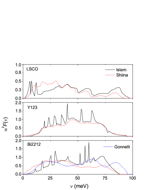
Figure 1: (color online) EPI spectral density $\alpha^{2}\emph{F}(\nu)$ for LSCO, Y123 and Bi2212. The black solid lines correspond to the method of Ref. Islam00, . The other lines are shown for comparison employing the methods of Ref. Shiina90, in all materials (dashed lines), and from Ref. Gonnelli98, in Bi2212 (dotted lines).

At this point, we should comment that other choices of the spectral density are possible, but have been left aside. For instance, the absence of the magnetic-resonance mode in LSCO and its appearance only below $T_{c}$ in some CSC are not consistent with the idea that the nodal kink has a magnetic origin. Zhou07 Along the same line, the reported absence of the magnetic-resonance mode in Bi2212 at a doping level of 0.23 without the disappearance of the superconducting stateHwang04 ($T_{c}\approx 55K$) reveals that the magnetic-resonance mode cannot be directly related to the spectral density involved in Eq. (1). Therefore, we have preferred the spectral densities oriented to phonons.

An important ingredient of our model is the commonly used dimensionless electron-phonon coupling parameter, defined in terms of the EPI spectral function by $\lambda\equiv 2\int_{0}^{\infty}d\nu\,\alpha^{2}F(\nu)/\nu$. This quantity is not to be straightforwardly identified with the mass-enhancement parameter $\lambda^{*}$. As it will be shown below, coincidence is only warranted under certain limits. A further relevant feature to mention is that $|g_{\textbf{k}\textbf{k}^{\prime}}^{j}|^{2}$ and as a consequence $\lambda$ are inversely proportional to the number of charge carriers contributed by each atom of the crystal to the bosonic coupling mode. Therefore, an increase in the doping level, which causes an increment in the hole concentration of the $CuO_{2}$ plane must be reflected in a reduction of $\lambda$ as we will see in the analysis of the kink structure. Furthermore, recalling the outstanding feature of the theory of metals, that $|g_{\textbf{k}\textbf{k}^{\prime}}^{j}|^{2}$ vanishes linearly with $|\textbf{k}-\textbf{k}^{\prime}|$ when $|\textbf{k}-\textbf{k}^{\prime}|\ll{k}_{F}$,Ashcroft76 one would expect a linear disappearance of the coupling effect that gives rise to the nodal kink in the vicinity of the Fermi surface. On the other hand, inspired by recent results on the universality of the nodal Fermi velocity $v_{F<}$ (at low energies) in certain cuprates, a prominent role of this quantity is also expected.

II.1 Green’s function formalism

Some words are due, considering Eq.(1) and the relation between the dressed and bare energies. Within the arguments customarily used for analyzing ARPES data, one finds the low energy approximation (close to the Fermi surface) $E_{k}\approx\varepsilon_{k}/(1+\lambda)$, with $\lambda$ the electron-phonon coupling parameter defined above. However, one should recall that such expression is an asymptotic form of the more correct $E_{k}\approx\varepsilon_{k}/(1+\lambda^{*})$ with $\lambda^{*}$ the true mass-enhancement parameter and $\lambda$ an appropriate limiting value. As a central result of our work, distinction between them is essential for the overall description of available data. Let us show how this arises.

Following the thermal Green’s function formalism, we assume that the electron-phonon interaction is introduced by the relation

$$G^{-1}(k,i\omega_{n})=G_{0}^{-1}(k,i\omega_{n})-\Sigma(k,i\omega_{n})$$ (3)

with $G_{0}^{-1}$ related to the bare electron energy and $i\omega_{n}$ standing for the “imaginary Matsubara frequencies”.Allen78

We recall that, technically, the bare electron band energy $\varepsilon_{k}$ is determined by the poles of the Green function $G(k,i\omega_{n})$, or the zeros of $G^{-1}(k,i\omega_{n})$ at the $i\omega_{n}$ frequencies.Allen78 On the other hand, it is known that additional dynamical information is contained in the analytic continuation $G(k,\omega+i0^{+})$ to points just above the real frequency axis, known as the “retarded” Green’s function. One is therefore led to continue the electronic self-energy $\Sigma(k,\omega+i0^{+})$ analytically by $\Sigma(k\omega+i0^{+})\equiv\Sigma_{1}(k,\omega)+i\Sigma_{2}(k,\omega)$. Now, suppose that a pole occurs near $\omega=0$ so, one gets

$$G^{-1}(k,\omega+i0^{+})=\omega-\varepsilon_{k}-\Sigma_{1}(k,\omega)-i\Sigma_{2}(k,\omega)$$ (4)

$$\simeq\omega\left(1-\left.\frac{\partial\Sigma_{1}(k,\omega)}{\partial\omega}\right|_{\omega=0}\right)-\left[\varepsilon_{k}+\Sigma_{1}(k,0)\right]-i\Sigma_{2}(k,\omega)\;.$$

Then, the pole of $G$ occurs at a frequency $\omega_{0}$ given by $\omega_{0}=E_{k}-i/2\tau_{k}$, with $\tau_{k}^{-1}=-2\left(1-\partial_{\omega}\Sigma_{1}\right)^{-1}\Sigma_{2}(k,E_{k})$ and

$$E_{k}=(1-\partial_{\omega}\Sigma_{1})^{-1}\left[\varepsilon_{k}+\Sigma_{1}(k,0)\right]\;.$$ (5)

Here $\lambda_{k}^{*}\equiv\left.-\partial_{\omega}\Sigma_{1}\right|_{\omega=0}$ is the technically defined mass-enhancement parameter.Allen82

We want to emphasize that replacement of $\lambda^{*}$ by $\lambda$ in Eq.(5) is only warranted for states $k$ at or very close to the Fermi surface when the ME approach for the self-energy [Eq.(1)] has been employed at the low temperature limit ($T\to 0$). Again, owing to the difficulties for evaluating $\Sigma_{1}$ beyond the Migdal approximation, our position in this paper has been to obtain $\lambda^{*}$ through the systematic evaluation of ARPES data, as shown in Sec.II.2. As a further detail, related to the limitations introduced by the use of the electron-phonon coupling parameter, one should mention that, long before the advent of the high $T_{c}$ superconductivity, Ashcroft and Wilkins showed that in some simple metals the single parameter $\lambda$ is insufficient to determine a number of thermodynamic properties such as the specific heat. Ashcroft65

In the following, we will introduce the simplest correction possible, for dealing with the correct mass-enhancement parameter. Noteworthily, it will be shown that a phenomenological linear relation, i.e.: $\lambda^{*}\simeq\delta\lambda$ suffices for the interpolation of experiments and numerical data. The physical interpretation of the parameter $\delta$ will be discussed within the following section (II.2). Just from the technical side, we want to comment that the mathematical material within this section has been developed using the convention of positive energy bands relative to the Fermi surface. It is apparent that the contrary selection can also be done, changing signs within intermediate expressions but the same final results, i.e.: $E_{k}=(1+\partial_{\omega}\Sigma_{1})^{-1}\left[\varepsilon_{k}-\Sigma_{1}(k,0)\right]$, with $\varepsilon_{k}$ defining negative energy bands.

II.2 Phenomenological dispersion relation

Let us make some final remarks before moving onto the application of the above ideas to the analysis of the ARPES data. Let us start by recalling that the bare electron band energy $\varepsilon_{k}$ is not directly available from the experiments. Instead, the electron momentum dispersion curve $E_{k}(k-k_{F})$ may be measured. However, it has been noted that the relation between the dressed and bare energies is a central property as related to the kink structure. In fact, based on the commonly used equation $E_{k}=\varepsilon_{k}+Re\{\Sigma(E_{k})\}$ one can consider that $\varepsilon_{k}$ implicitly depends on $E_{k}$ through the boson coupling parameter $\lambda$.Schachinger03 ; Giustino08 This fact, along with some ansatz for the ARPES “bare” dispersion allows to obtain $\lambda$ as a unique constrained parameter that better fits the observed kink structure. However, the indiscriminate proposal of dispersion relations could considerably under or overestimate the average renormalization because implicit approximations are used as indicated in the previous section. Furthermore, we stress that, the use of the same ansatz on different cuprates or even for a definite material with slight variations in the doping level is not warranted. In this work, with the aim of finding a widespread renormalization function that describes the behavior of the kink in different CSC and for different doping levels, we have carried out an exhaustive study on the incidence of the EPI coupling parameter in the appearance of kink-dispersion. Based on an interpolation scheme between the numerical behavior of the relation $E_{k}=\varepsilon_{k}+Re\{\Sigma(E_{k})\}$ and the experimental data, as a central result, we have encountered that the practical totality of data are accurately reproduced by a universal dispersion relation of the kind

$${k}-{k}_{F}=\frac{\varepsilon_{k}}{v_{F_{<}}}\left(1-\frac{\varpi}{\omega_{\rm log}}\lambda\right)\,,$$ (6)

with $v_{F_{<}}$ the Fermi velocity at low-energies, $\omega_{\rm log}$ the so-called logarithmic frequency as introduced by Allen,Allen75 and $\varpi$ the (only) free parameter required for incorporating the specific renormalization for each superconductor. Note that the constant frequency $\omega_{\rm log}$ (properly defining the corresponding spectral densities $\alpha^{2}F(\nu)$ for each $\lambda$) has been introduced only for scaling purposes, just with the aim of reducing the scattering of numerical values in dealing with different samples. In this sense, $\varpi$ is a mere mathematical instrument. Thus, our numerical program is as follows: (i) $v_{F_{<}}$ is determined from the momentum dispersion curve in the ARPES measurements [$\sim$ 1.4 eVÅ - 2.2 eVÅ], (ii) $\omega_{\rm log}$ is evaluated from the spectral densities shown in Fig.1 through the definition $\omega_{\rm log}\equiv exp\{(2/\lambda)\int_{0}^{\infty}\ln(\nu)[{\alpha^{2}F(\nu)}/{\nu}]d\nu\}$ (we get $\omega_{\rm log}^{LSCO}\simeq 16.1455\,meV$, $\omega_{\rm log}^{Y123}\simeq 35.5900\,meV$ and $\omega_{\rm log}^{Bi2212}\simeq 33.8984\,meV$ respectively), (iii) $\varepsilon_{k}$ is numerically determined from the relation $E_{k}=\varepsilon_{k}+Re\{\Sigma(E_{k})\}$, and (iv) correlation is established between theory and experiment by the application of Eq.(6).

From the physical point of view, our empirical ansatz [Eq.(6)] may interpreted as follows. Let us assume that the involved quantities are not far from their values at the Fermi level, and start with $\varepsilon_{k}$ replaced by $E_{k}-\Sigma_{1}(E_{k})$, i.e.

$$E_{k}-\Sigma_{1}(E_{k})=\left({k}-{k}_{F}\right)v_{F_{<}}\left(1-\delta\lambda\right)^{-1}\,,$$ (7)

where the definition $\delta\equiv{\varpi}/{\omega_{\rm log}}$ has been used. Now, let us take derivatives respect to $E_{k}$ and evaluate for $E_{k}\to 0$. One gets

$$1+\lambda^{*}=\left.\frac{\partial(k-k_{F})}{\partial E_{k}}\right|_{E_{k}=0}v_{F<}(1-\delta\lambda)^{-1}\,,$$ (8)

and recalling that $v_{F<}$ is obtained as the slope of the lower part of the momentum dispersion curve,Zhou03 this equation leads to $1+\lambda^{*}=(1-\delta\lambda)^{-1}$. Thus, a physical interpretation of the fit parameter $\delta$ is obtained, i.e.: $\delta=(\lambda^{*}/\lambda)/(1+\lambda^{*})$. To the lowest order, the dimensionless parameter $\delta$ is basically the ratio between the defined mass-enhancement and phonon-coupling parameters $\delta\approx\lambda^{*}/\lambda$. Outstandingly, it will be shown that this fact reassembles the differences obtained by tight-binding Hamiltonian models Weber87 ; Weber88 and the “density-functional” band theories Giustino08 ; Heid08 . Recall that, in principle, the density-functional theory Kohn66 gives a correct ground-state energy, but the bands do not necessarily fit the quasi-particle band structure used to describe low-lying excitations. As it will be seen below, predictions from both types of models may be reconciled appealing to the differences between $\lambda$ and $\lambda^{*}$.

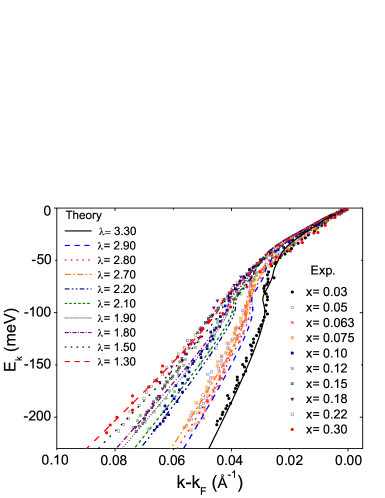
Figure 2: (color online) The renormalized energy $E_{k}$ as a function of momentum $k-k_{F}$ for $La_{2-x}Sr_{x}CuO_{4}$ with various doping levels between 0.03 (right curve) and about 0.30 (left curve), all measured at a temperature of $20K$ along the nodal direction. Experimental data are taken from Ref. Zhou03, . The theoretical curves are labeled according to the best fit values for $\lambda$.

Table 1: Values of the boson-coupling parameter $\lambda$ and the corresponding mass-enhancement parameter $\lambda^{*}$ obtained from the analysis of ARPES data at several doping levels of $La_{2-x}Sr_{x}CuO_{4}$. $\lambda^{*}$ has been obtained by means of Eq. (6) to the lowest order $\lambda^{*}\approx\delta\lambda$ (in this case $\delta=0.185$). The predicted superconducting transition temperatures $T_{c}$ are also shown. Our results are presented in contrast with other models available in the literature.

SC	$x$	Ref.	$\lambda$	$\lambda^{*}$	$T_{c}(\lambda)$ [K]
LSCO	0.03	This	3.30	0.61	–
	0.05		2.90	0.54	–
	0.063		2.80	0.52	–
	0.075		2.70	0.50	–
	0.10		2.20	0.41	42.10
	0.12		2.10	0.39	40.77
	0.15		1.90	0.35	37.83
	0.18		1.80	0.33	36.19
	0.22		1.50	0.28	30.47
	0.30		1.30	0.24	–
	0.1-0.2	[Weber87, ]	2-2.5	–	30 - 40
	–	[Shiina90, ]	1.78	–	40.6
	0.15	[Giustino08, ]	1 - 1.32	0.14 - 0.22	–
	0.22	[Giustino08, ]	0.75 - 0.99	0.14 - 0.20	–

III Analysis of ARPES data

Below, we present the application of our theoretical analysis for a wide set of experimental curves available in the literature. The main facts are shown in figures 2- 4, and summarized in tables 1-3.

Results for LSCO.–

In Fig. 2 we show the results found in $La_{2-x}Sr_{x}CuO_{4}$ covering the doping range ($0<x\leq 0.3$). Remarkably, within this range, the physical properties span over the insulating, superconducting, and overdoped non-superconducting metal behavior. Superconducting transition temperatures $T_{c}$ in the interval of 30-40K have been observed by Bednorz and Müller Bednorz86 and others Uchida87 ; Dietrich87 . For the application of Eq.(6), here, we have considered $v_{F_{<}}=2eV\cdot$Å as related to the experimental results of Refs. Zhou07, ; Lanzara01, ; Zhou03, ; Zhou05, . On the other hand, the best fit of the whole set of experimental data has been obtained for $\delta=0.185$, and the derived $\lambda^{*}$ values are shown in the Table 1. For comparison, recall that values of “$\lambda=2-2.5$” in the range $0.2>x>0.1$ were reported in the Ref. Weber87, by Weber. In that case they were obtained within the framework of the nonorthogonal-tight-binding theory of lattice dynamics, based on the energy band results of Mattheiss Mattheiss87 and corresponding to the range of the EPI coupling parameter $\lambda$ predicted in our model. It must be emphasized that in the case of Ref. Weber87, , $\lambda$ was obtained in agreement with the observed $T_{c}$ values in LSCO. Moderate discrepancies between the predictions of our phenomenological model and the analysis of Refs. Weber87, and Weber88, may be ascribed to some uncertainty in the experimental spectral densities. As regards the critical temperatures, we have calculated them based on the celebrated McMillan’s equation,McMillan68 $T_{c}=(\omega_{log}/1.2)exp[-1.04(1+\lambda)/(\lambda-\mu^{*}(1+0.62\lambda))]$ (see table 1). In all the calculations, the Coulomb’s pseudopotencial was given a typical value, $\mu^{*}=0.13$. It is essential to be aware that, there is no small parameter which enables a satisfactory perturbation theory to be constructed for the Coulomb interaction between electrons. Thus Coulomb contributions to the electron self-energy $\Sigma$ cannot be reliably calculated.Allen75 Fortunately this is not a serious problem in superconductivity because a reasonable assumption is to consider that the large normal-state Coulomb effects contained in the Coulomb self-energy are already included in the bare band structure $\varepsilon_{k}$. The remaining off-diagonal terms of the superconducting components of the Coulomb self-energy turn out to have only a small effect on superconductivity, which is treated phenomenologically.Allen82 One can see that the consideration of the electron-phonon interaction in LSCO strongly suggests that the high $T_{c}$ values can be caused by conventional electron-phonon coupling, in agreement with the conclusion of Weber. Weber87

From a different perspective, in a recent publication, Giustino and co-workersGiustino08 have calculated the electronic structure of LSCO employing a generalized gradient approximation to density functional theory (DFT). These authors have extracted the “$\lambda$” parameter by measuring the gradients of both the theoretical and the experimental Lanzara01 self-energy data within the low energy limit ($0-50meV$). Their procedure yields $\lambda_{expt}=1.00-1.32$ for the optimally doped sample ($x=0.15$) at 20K and $\lambda_{expt}=0.75-0.99$ for the overdoped sample ($x=0.22$) while the theoretical results $\lambda_{th}=0.14-0.22$ at optimal doping and $\lambda_{th}=0.14-0.20$ in the overdoped regime. It is concluded that theoretical values noticeably underestimate the experiments and, thus, that the electron-phonon interaction is unlikely to be relevant in LSCO. From our view, considering that the theoretical value is calculated from the gradient of the DFT self-energy, $\lambda_{th}$ is basically to be identified with $\lambda^{*}$, while $\lambda_{expt}$ matches the electron-phonon coupling $\lambda$ involved in the standard Migdal formalism analysis of experiments.

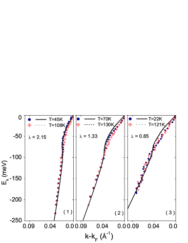
Figure 3: (color online) Same as in Fig. [2] but in samples of $Bi_{2}Sr_{2}CaCu_{2}O_{8+x}$ with (left to right):$x=0.12$ (underdoped), $x=0.16$ (optimally doped), and $x=0.21$ (overdoped). The red diamonds and blue circles correspond to the experimental data of Ref. Johnson01, . The continuous lines correspond to our theoretical curves.

Table 2: Same as table 1 but for the case of $Bi_{2}Sr_{2}CaCu_{2}O_{8+x}$.Here, several values of $\lambda$ are not related to ARPES data, but just introduced for comparison. In this case, $\delta=0.354$

SC	$x$	Ref.	$\lambda$	$\lambda^{*}$	$T_{c}(\lambda)$ [K]
Bi2212	0.12	This	2.15	0.76	64.81
	0.16		1.33	0.47	42.45
	0.21		0.85	0.30	19.93
	–	[Shiina90, ]	3.28	–	85
	–	This	3.28	1.16	81.66
	–	[Gonnelli98, ]	3.34	1.05	93
	–	This	3.34	1.18	82.40
	0.16	[Kordyuk06, ]	$\sim 1.28$	$\sim 0.43$	–

Results for BSCCO.–

In Fig. 3 we display the results found in samples of Bi2212. Each case has been studied with temperatures both in the normal and superconducting state. The experimental data were taken from the work by Johnson et al.Johnson01 In this case, we have used $v_{F_{<}}=1.6eV\cdot$Å as a value consistent with the experimental results of Refs. Lanzara01, ; Kordyuk06, ; Zhou02, ; Johnson01, . The best fit with experimental data has been found for $\delta=0.354$. Similarly to the case of LSCO, our analysis fits well the “$\lambda$” values predicted by others and very different models Shiina90 ; Gonnelli98 ; Kordyuk06 (see table 2). From our results, it is clear that the phonon coupling mode as a unique source for the behavior of the critical temperature in BSCCO is only reasonable for the underdoped case (x=0.12). Nevertheless, the full energy spectrum in the nodal direction and the consequent emergence of the kink-effect are reproduced.

Results for YBCO.–

Finally, in Fig. 4 we show the results found for Y123 samples. The experimental data were taken from recent work by Borisenko et al.Borisenko06 To our knowledge, no more experimental evidence of kinks in the nodal direction is available for Y123. The value $v_{F_{<}}=1.63eV\cdot$Å has been used for consistency with the experimental results reported by those authors. The best fit between the experimental data and our model has been found with the value $\delta=0.365$. It must be noted that the appearance of a second kink in the underdoped case may not be allocated in the current model, and requires further theoretical considerations. Contrary to the properties of the overdoped case, that is captured by the theory in the full energy spectrum, the underdoped case is only reproduced at low energies (1st kink close to the Fermi level). One possibility for upgrading the theory would be to consider the existence of additional contributions to the electron self-energy $\Sigma$ which could be related to high orders of the phonon perturbation, vertex corrections, or inclusive Coulombian effects. On the other hand, one specific feature of Y123 is that, contrary to the other superconductor cuprates, the reservoir layers in these materials contain $CuO$ chain layers which could be contributing significantly to the band energies of the in-plane electronic structure. This hypotheses has been used with success by Cucolo et al. Cucolo96 for the interpretation of tunneling spectra, specific heat and the ultrasonic attenuation coefficient in both phases of Y123. More detailed studies on the electronic photoemission spectra of Y-based copper oxides are required. Unfortunately on the basis of the existing data, then, it is not possible to favor one or other of these possibilities. Moreover, in ARPES one should also care about the residual 3-dimensionality and its effect on photoemission data. Again, our model fits well the “$\lambda$” values predicted by other works Shiina90 ; Weber88 ; Heid08 (see table 3). However, is clear that the phonon coupling mode as the source for the critical temperature in YBCO samples is not reasonable. The same conclusion has already been obtained in the Refs. Weber88, and Heid08, .

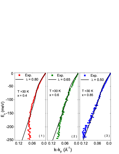
Figure 4: (color online) Same as in Fig. [2] but in samples of $YBa_{2}Cu_{3}O_{6+x}$ with (left to right): $x=0.4$ (underdoped), $x=0.6$ (underdoped), and $x=0.85$ (overdoped). The solid squares correspond to the experimental data of Ref. Borisenko06, . The lines correspond to our theoretical curves. All curves have been obtained at 30K.

Table 3: Same as tables 1 and 2 but for $YBa_{2}Cu_{3}O_{6+x}$ samples. In this case, $\delta=0.365$

SC	$x$	Ref.	$\lambda$	$\lambda^{*}$	$T_{c}(\lambda)$ [K]
YBCO	0.4	This	0.80	0.29	17.51
	0.6		0.65	0.24	9.82
	0.85		0.50	0.18	3.39
	–	[Shiina90, ]	$\sim$3.4	–	91
	–	This	3.45	1.26	84.19
	–	[Weber88, ]	$\sim$0.5	–	$\sim$3
	–	[Weber88, ]	$\sim$1.3	–	$\sim$30
	–	This	1.30	0.47	36.43
	–	[Heid08, ]	–	0.18 - 0.22	–
	–	This	0.49 - 0.60	0.18 - 0.22	$\sim$3.0 - 6.6

IV Concluding remarks

In summary, we have introduced a model that allows to reproduce the appearance of the ubiquitous nodal kink for a wide set of ARPES experiments in cuprate superconductors. Our proposal is grounded on the Migdal-Eliashberg approach for the self-energy of quasi-particles within the electron-phonon coupling scenario. The main issue is the proposal of a linear dispersion relation for the bare band energy, i.e.: $\varepsilon_{k}=(k-k_{F})v_{F<}(1-\delta\lambda)^{-1}$. $\delta$, the only free parameter of the theory is a universal property for each family of cuprates. It has been interpreted as the relation between the mass-enhancement $\lambda^{*}$ and electron-phonon coupling $\lambda$ parameters.

An excellent agreement between the theory and the available collection of experiments is achieved. Our results support the idea that the phonon coupling mechanism is the main cause of the kink effect and the so-called universal nodal Fermi velocity, although its effect in the appearance of the superconducting state and the high critical temperatures is not clear yet.

For decades, a well-known controversy has arisen on the role of the parameter “$\lambda$” whose values noticeably scatter among different model calculations. As a central result, our proposal re-ensembles the “$\lambda$” values obtained from different models and, as a first approximation, solves the controversy through the relation $\lambda^{*}\cong\delta\lambda$. We emphasize that the phenomenological parameter $\delta$ (obtained through the analysis of a wide collection of data) has allowed to go beyond the conventional Migdal-Eliashberg approach analysis of restricted sets of experiments.

Our model is directly supported by the “$\lambda$” values obtained in Refs. Shiina90, ; Gonnelli98, ; Giustino08, ; Kordyuk06, ; Heid08, ; Weber87, ; Weber88, . When inserted into the celebrated McMillan’s formula these values indicate that the electron-phonon coupling behind is not necessarily the only mechanism responsible for the superconducting properties of all the cuprates. In fact, the critical temperatures that one can calculate are only at reasonable levels for the case of LSCO (table 1) and for underdoped BSCCO (Table 2) where the phonon mechanism dominates.

References

- (1) S. Hüfner (Ed.), Very High Resolution Photoelectron Spectroscopy (Springer, Berlin, 2007).
- (2) X. J. Zhou, T. Cuk, T. Devereaux, N. Nagaosa, and Z.-X. Shen Handbook of High-Temperature Superconductivity (Springer, New York, 2007), chap. 3, p. 87.
- (3) A. Damascelli, Z. Hussain and Z.-X. Shen, Rev. Mod. Phys. 75, 473 (2003).
- (4) J. C. Campuzano, M. R. Norma and M. Randeria in Physics of Superconductors, edited by K. H. Bennemann and J. B. Ketterson (Springer, Berlin, 2004), Vol. II, p. 167-273.
- (5) M. Randeria , H. Ding, J. C. Campuzano, A. Bellman, G. Jennings, T. Yokoya, T. Takahashi, H. Katayama-Yoshida, T. Mochiku, and K. Kadowaki, Phys. Rev. Lett. 74, 4951 (1995).
- (6) L. Hedin and J. D. Lee, J. Electron Spectrosc. Relat. Phenom. 124, 289 (2002).
- (7) J. D. Koralek, J. F. Douglas, N. C. Plumb, Z. Sun, A. V. Fedorov, M. M. Murnane, H. C. Kapteyn, S. T. Cundiff, Y. Aiura, K. Oka, H. Eisaki, and D. S. Dessau, Phys. Rev. Lett. 96, 017005 (2006).
- (8) X. J. Zhou, Z. Hussain, and Z.-X. Shen, J. Electron Spectrosc. Relat. Phenom. 126, 145 (2002).
- (9) A. Lanzara, P. V. Bogdanov, X. J. Zhou, S. A. Kellar, D. L. Feng, E. D. Lu, T. Yoshida, H. Eisaki, A. Fujimori, K. Kishio, J.-I. Shimoyama, T. Noda, S. Uchida, Z. Hussain, and Z.-X. Shen, Nature 412, 510 (2001).
- (10) X. J. Zhou, T. Yoshida, A. Lanzara, P. V. Bogdanov, S. A. Kellar, K. M. Shen, W. L. Wang, F. Ronning, T. Sasagawa, T. Kakeshita, T. Noda, H. Eisaki, S. Uchida, C. T. Lin, F. Zhou, J. W. Xiong, W. X. Ti, Z. X. Zhao, A. Fujimori, Z. Hussain, and Z.-X. Shen, Nature 423, 398 (2003).
- (11) X. J. Zhou, Junren Shi, T. Yoshida, T. Cuk, W. L. Yang, V. Brouet, J. Nakamura, N. Mannella, Seiki Komiya, Yoichi Ando, F. Zhou, W. X. Ti, J. W. Xiong, Z. X. Zhao, T. Sasagawa, T. Kakeshita, H. Eisaki, S. Uchida, A. Fujimori, Zhenyu Zhang,E. W. Plummer, R. B. Laughlin, Z. Hussain, and Z.-X. Shen, Phys. Rev. Lett. 95, 117001 (2005).
- (12) A. A. Kordyuk, S. V. Borisenko, V. B. Zabolotnyy, J. Geck, M. Knupfer, J. Fink, B. Büchner, C. T. Lin, B. Keimer, H. Berger, A. V. Pan, S. Komiya, and Y. Ando, Phys. Rev. Lett. 97, 017002 (2006).
- (13) Y. X. Xiao, T. Sato, K. Terashima, H. Matsui, T. Takahashi, M. Kofu, and K. Hirota, Physica C 463-465, 44 (2007).
- (14) T. Takahashi, Physica C 460-462, 198 (2007).
- (15) G.-H. Gweon, T. Sasagawa, S. Y. Zhou, J. Graf, H. Takagi, D.-H. Lee, and A. Lanzara, Nature 430, 187 (2004).
- (16) J. F. Douglas, H. Iwasawa, Z. Sun, A. V. Fedorov, M. Ishikado, T. Saitoh, H. Eisaki, H. Bando, T. Iwase, A. Ino, M. Arita, K. Shimada, H. Namatame, M. Taniguchi, T. Masui, S. Tajima, K. Fujita, S. Uchida, Y. Aiura, and D S. Dessau, Nature 446, E5 (2007).
- (17) P. D. Johnson, T. Valla, A. V. Fedorov, Z. Yusof, B. O. Wells, Q. Li, A. R. Moodenbaugh, G. D. Gu, N. Koshizuka, C. Kendziora, Sha Jian, and D. G. Hinks, Phys. Rev. Lett 87, 177007 (2001).
- (18) S. V. Borisenko, A. A. Kordyuk, V. Zabolotnyy, J. Geck, D. Inosov, A. Koitzsch, J. Fink, M. Knupfer, B. Büchner, V. Hinkov, C. T. Lin, B. Keimer, T. Wolf, S. G. Chiuzbăian, L. Patthey, and R. Follath, Phys. Rev. Lett 96, 117004 (2006).
- (19) P. B. Allen and B. Mitrović, in Solid State Physics, edited by H. Ehrenreich, F. Seitz, and D. Turnbull (Academic, New York, 1982), Vol. 37, p. 1.
- (20) H. S. Ruiz, J. J. Giraldo, and R. Baquero, J. Supercond. Nov. Magn. 21, 21 (2008).
- (21) A. T. M. N. Islam and A. K. M. A. Islam, J. Supercond. 13, 559 (2000).
- (22) B. Renker, I. Apfelstedt, H. Küpfer, C. Politis, H. Rietschel, W. Schauer, H. Wühl, U. Gottwick, H. Kneissel, U. Rauchschwalbe, H. Spille, and F. Steglich, Z. Phys. B 67, 15 (1987).
- (23) B. Renker, F. Gompf, D. Ewert, P. Adelmann, H. Schmidt, E. Gering and H. Mutka, Z. Phys. B 77, 65 (1989).
- (24) B. Renker, F. Gompf, E. Gering, D. Ewert, H. Rietschel, and A. Dianoux, Z. Phys. B 73, 309 (1988).
- (25) Y. Shiina and Y. O. Nakamura, Sol. State Commun. 76, 1189 (1990).
- (26) R. S. Gonnelli, G. A. Ummarino, and V. A. Stepanov, J. Phys. Chem. Solids 59, 2058 (1998).
- (27) J. Hwang, T. Timusk, and G. D. Gu, Nature 427, 714 (2004).
- (28) N. W. Ashcroft and N. D. Mermin, Solid State Physics (Saunders College Publishing, 1976), chap. 26, p. 521.
- (29) P. B. Allen, Phys. Rev. B 18, 5217 (1978).
- (30) N. W. Ashcroft and J. W. Wilkins, Physics Lett. 14, 285 (1965).
- (31) E. Schachinger, J. J. Tu, and J. P. Carbotte, Phys. Rev. B. 67, 214508 (2003).
- (32) F. Giustino, M. L. Cohen, and S. G. Louie, Nature 452, 975 (2008).
- (33) P. B. Allen and R. C. Dynes, Phys. Rev. B 12, 905 (1975).
- (34) W. Weber, Phys. Rev. Lett. 58, 1371 (1987).
- (35) W. Weber, Phys. Rev. B. (Rapid Comm.) 37, 599 (1988).
- (36) R. Heid, K.-P Bohnen, R. Zeyher, and D. Manske Phys. Rev. Lett. 100, 137001 (2008).
- (37) W. Kohn, in “Many Body Theory” (R. Kubo, ed.), p. 73. Syokabō, Tokio, 1966.
- (38) J. G. Bednorz and K. A. Müller, Z. Phys. B 64, 18 (1986).
- (39) S. Uchida, H. Takagi, K. Kishio, K. Kitazawa, K. Fueki, and S. Tanaka, Jpn. J. Appl. Phys. 26, L443 (1987).
- (40) M. R. Dietrich, W. H. Fietz, J. Ecke, B. Obst and C. Politis, Z. Phys. B 66, 283 (1987).
- (41) L. F. Mattheiss, Phys. Rev. Lett. 58, 1028 (1987).
- (42) W. L. McMillan, Phys. Rev. 167, 331 (1968).
- (43) A. A. Kordyuk, S. V. Borisenko, A. Koitzsch, J. Fink, M. Knupfer, and H. Berger, Phys. Rev. B. 71, 214513 (2005).
- (44) A. M. Cucolo, C. Noce, and A. Romano, Phys. Rev. B 53, 6764 (1996).