Observation of $B^{0}\to{\Lambda\bar{\Lambda}K^{0}}$ and $B^{0}\to{\Lambda\bar{\Lambda}K^{*0}}$ at Belle

Abstract

We study the charmless decays $B\to\Lambda\bar{\Lambda}h$, where $h$ stands for $\pi^{+}$, $K^{+}$, $K^{0}$,$K^{*+}$, or $K^{*0}$, using a $605\,{\rm fb}^{-1}$ data sample collected at the $\Upsilon(4S)$ resonance with the Belle detector at the KEKB asymmetric energy $e^{+}e^{-}$ collider. We observe $B^{0}\to{\Lambda\bar{\Lambda}K^{0}}$ and $B^{0}\to{\Lambda\bar{\Lambda}K^{*0}}$ with branching fractions of $(4.76^{+0.84}_{-0.68}(stat.)\pm 0.61(syst.))\times 10^{-6}$ and $(2.46^{+0.87}_{-0.72}\pm 0.34)\times 10^{-6}$, respectively. The significances of these signals in the threshold-mass enhanced mass region are $12.4\sigma$ and $9.3\sigma$, respectively. We also update the branching fraction $\mathcal{B}(B^{+}\to{\Lambda\bar{\Lambda}K^{+}})=(3.38^{+0.41}_{-0.36}\pm 0.41)\times 10^{-6}$ with better accuracy, and report the following measurement or 90% confidence level upper limit in the threshold-mass-enhanced region: $\mathcal{B}(B^{+}\to{\Lambda\bar{\Lambda}K^{*+}})=(2.19^{+1.13}_{-0.88}\pm 0.33)\times 10^{-6}$ with 3.7$\sigma$ significance; $\mathcal{B}(B^{+}\to{\Lambda\bar{\Lambda}\pi^{+}})<0.94\times 10^{-6}$. A related search for $B^{0}\to\Lambda\bar{\Lambda}\bar{D}^{0}$ yields a branching fraction $\mathcal{B}(B^{0}\to\Lambda\bar{\Lambda}\bar{D}^{0})=(1.05_{-0.44}^{+0.57}\pm 0.14)\times 10^{-5}$. This may be compared with the large, $\sim 10^{-4}$, branching fraction observed for $B^{0}\to{p\bar{p}}\bar{D^{0}}$. The $M_{\Lambda\bar{\Lambda}}$ enhancements near threshold and related angular distributions for the observed modes are also reported.

PACS: 13.25.Hw, 14.40.Nd

I Introduction

The $b\to s$ penguin loop process plays an important role in rare $B$ meson decays MEPeskin . It could be sensitive to new physics beyond the standard model due to additional contributions from as yet-unknown heavy virtual particles in the loop. Recently the study of the penguin dominated baryonic $B$ decays $B^{+}\to{p\bar{p}K^{+}}$ Wei and $B^{0}\to{p\bar{\Lambda}\pi^{-}}$ Wang gave intriguing results. The proton polar angular distributions in the baryon-antibaryon helicity frame disagree with the expectations for short distance $b\to s$ weak decays Suzuki07 . However, in $B\to{p\bar{p}}K^{*}$ decays JHChen , the ${K^{*0}}$ seems to be fully polarized in the helicity zero state in agreement with the $b\to s$ weak decay hypothesis. The theoretical hierarchies, $\mathcal{B}(B^{+}\to{p\bar{p}K^{+}})>\mathcal{B}(B^{+}\to{p\bar{p}K^{*+}})$ and $\mathcal{B}(B^{+}\to{p\bar{p}K^{*+}})>\mathcal{B}(B^{0}\to{p\bar{p}K^{*0}})$, from the pole model HYCheng are experimentally established although the predicted branching fraction $\mathcal{B}(B^{0}\to{p\bar{p}K^{*0}})$ is about a factor of 20 smaller than the experimental measurement. It is therefore interesting to study the corresponding branching fractions for $B\to\Lambda\bar{\Lambda}K^{(*)}$ decays, the counterparts with protons replaced by $\Lambda$’s.

In this paper, we study the charmless three-body decays $B\to\Lambda\bar{\Lambda}h$, where $h$ stands for $\pi^{+}$, $K^{+}$, $K^{0}$, $K^{*+}$, or $K^{*0}$ conjugate . The mode $B^{+}\to{\Lambda\bar{\Lambda}K^{+}}$ has been previously observed YJLee and presumably proceeds through a $\bar{b}\to\bar{s}s\bar{s}$ process. This decay process can be related to $B^{+}\to{p\bar{p}K^{+}}$ as shown in Fig. 1(a) and Fig. 1(b). One can simply replace the $ud-\bar{u}\bar{d}$ diquark pair with an $sd-\bar{s}\bar{d}$ pair to establish a one-to-one correspondence between $B\to{p\bar{p}}h$ and $\Lambda\bar{\Lambda}h$ decays. A common feature of these decays is that the baryon-antibaryon mass spectra peak near threshold as conjectured in Refs. Suzuki07 ; HS . The $K^{+}$ meson carries the energetic $\bar{s}$ quark from the $\bar{b}\to\bar{s}$ transition so that a threshold enhancement of the baryon and antibaryon system is naturally formed. However, there is another possibility shown in Fig. 1(c) and Fig. 1(d), where the $\bar{\Lambda}$ (instead of the $K^{+}$) carries the $\bar{s}$ from the $\bar{b}\to\bar{s}$ transition. It is interesting to know the role of this $\bar{s}$ quark in $B\to\Lambda\bar{\Lambda}K^{(*)}$ weak decays.

Since the branching fractions of $B\to\Lambda\bar{\Lambda}K$ and ${\Lambda\bar{\Lambda}\pi^{+}}$ decays are theoretically expected at a level prediction that is detectable with our present data sample, we attempt to determine the branching fractions of the various $B\to\Lambda\bar{\Lambda}h$ decays and compare with the latest measurements for $B\to{p\bar{p}}h$. We also examine the low mass $M_{\Lambda\bar{\Lambda}}$ enhancements near threshold and the related angular distributions in order to investigate the underlying dynamics.

(a)                                                          (b)

(c)                                                          (d)

Figure 1: Comparisons of possible decay diagrams between $B^{+}\to{p\bar{p}K^{+}}$/$B^{0}\to{p\bar{\Lambda}\pi^{-}}$ and $B^{+}\to{\Lambda\bar{\Lambda}K^{+}}$.

II Event Selection and Reconstruction

II.1 Data Samples and the Belle Detector

For this study, we use a 605 fb^-1 data sample, consisting of 657 $\times 10^{6}B\bar{B}$ pairs, collected with the Belle detector on the $\Upsilon({\rm 4S})$ resonance at the KEKB asymmetric energy $e^{+}e^{-}$ (3.5 and 8 GeV) collider KEKB . The Belle detector is a large-solid-angle magnetic spectrometer that consists of a silicon vertex detector (SVD), a 50-layer central drift chamber (CDC), an array of aerogel threshold Cherenkov counters (ACC), a barrel-like arrangement of time-of-flight scintillation counters (TOF), and an electromagnetic calorimeter composed of CsI(Tl) crystals located inside a super-conducting solenoid coil that provides a 1.5 T magnetic field. An iron flux-return located outside of the coil is instrumented to detect $K_{L}^{0}$ mesons and to identify muons. The detector is described in detail elsewhere Belle .

II.2 Selection Criteria

The event selection criteria are based on information obtained from the tracking system (SVD and CDC) and the hadron identification system (CDC, ACC, and TOF). All charged tracks not associated with long lived particles are required to satisfy track quality criteria based on track impact parameters relative to the interaction point (IP). The deviations of charged tracks from the IP position are required to be within $\pm$0.3 cm in the transverse ($x$–$y$) plane, and within $\pm$3 cm in the $z$ direction, where the $z$ axis is defined to be the direction opposite to the positron beam. For each track, the likelihood values $L_{p}$, $L_{K}$, and $L_{\pi}$ for the proton, kaon, or pion hypotheses, respectively, are determined from the information provided by the hadron identification system. A track is identified as a kaon if $L_{K}/(L_{K}+L_{\pi})>0.6$, or as a pion if $L_{\pi}/(L_{K}+L_{\pi})>0.6$. This selection is about 86% (93%) efficient for kaons (pions) while removing about 96% (94%) of pions (kaons). ${K_{S}^{0}}$ candidates are reconstructed from pairs of oppositely charged tracks (both treated as pions) with an invariant mass in the range $485$ MeV/c${}^{2}<M_{\pi^{+}\pi^{-}}<510$ MeV/c². The dipion candidate must have a displaced vertex and flight direction consistent with a ${K_{S}^{0}}$ originating from the interaction point. We use the selected kaons and pions to form ${K^{*{+}}}$ ($\to{K_{S}^{0}}\pi^{+}$) and ${K^{*0}}$ ($\to K^{+}\pi^{-}$) candidates. Events with a $K^{*}$ candidate mass between 0.6 GeV/c² and 1.2 GeV/c² are used for further analysis. Similarly, we select $\Lambda$ baryons by applying the ${K_{S}^{0}}$ vertex displacement and flight direction selection criteria to pairs of oppositely charged tracks—treated as a proton and negative pion—whose mass is consistent with the nominal $\Lambda$ baryon mass, 1.111 GeV/c${}^{2}<M_{p\pi^{-}}<1.121$ GeV/c² lambdamass . The proton-like daughter is required to satisfy $L_{p}/(L_{p}+L_{\pi})>0.6$. This selection is about 97% (95%) efficient for protons (anti-protons) while removing about 99% of pions.

II.3 B Meson Reconstruction

Candidate $B$ mesons are reconstructed in the $B^{+}\to{\Lambda\bar{\Lambda}K^{+}}$, $B^{+}\to{\Lambda\bar{\Lambda}\pi^{+}}$, $B^{0}\to{\Lambda\bar{\Lambda}K^{0}}$, $B^{+}\to{\Lambda\bar{\Lambda}K^{*+}}$ and $B^{0}\to{\Lambda\bar{\Lambda}K^{*0}}$ modes. We use two kinematic variables in the center of mass (CM) frame to identify the reconstructed $B$ meson candidates: the beam energy constrained mass ${M_{\rm bc}}=\sqrt{E^{2}_{\rm beam}-p^{2}_{B}}$, and the energy difference ${\Delta{E}}=E_{B}-E_{\rm beam}$, where $E_{\rm beam}$ is the beam energy, and $p_{B}$ and $E_{B}$ are the momentum and energy, respectively, of the reconstructed $B$ meson. The candidate region is defined as 5.2 GeV/c${}^{2}<{M_{\rm bc}}<5.3$ GeV/c² and $-0.1$ GeV $<{\Delta{E}}<0.3$ GeV. The lower bound in ${\Delta{E}}$ for candidate events is chosen to exclude possible background from baryonic $B$ decays with higher multiplicities. From a GEANT geant based Monte Carlo (MC) simulation, the signal peaks in a signal box defined by the requirements 5.27 GeV/c${}^{2}<{M_{\rm bc}}<5.29$ GeV/c² and $|{\Delta{E}}|<0.05$ GeV. To ensure that the decay process be genuinely charmless, we apply a charm veto. The regions $2.850$ GeV/c${}^{2}<M_{\Lambda\bar{\Lambda}}<3.128$ GeV/c² and $3.315$ GeV/c${}^{2}<M_{\Lambda\bar{\Lambda}}<3.735$ GeV/c² are excluded to remove background from modes with $\eta_{c},J/\psi$ and $\psi^{\prime},\chi_{c0},\chi_{c1}$ mesons, respectively. According to a study of a rare $B$ decay MC sample, the backgrounds in all candidate regions due to self cross-feeds (e.g between $B^{+}\to{\Lambda\bar{\Lambda}K^{+}}$ and $B^{0}\to{\Lambda\bar{\Lambda}K^{*+}}$) or due to other rare decays such as $B^{0}\to{p\bar{\Lambda}\pi^{-}}$, etc., are negligible. The contribution of the $B$ background component with $\Sigma\to\gamma\Lambda$ is estimated by fitting the ${\Delta{E}}$ distribution. This will be included in the systematic uncertainty from fitting by comparing the results with and without this background component in the fit.

II.4 Background Suppression

After the above selection requirements, the background in the fit region arises dominantly from continuum $e^{+}e^{-}\to q\bar{q}$ ($q=u,\ d,\ s,\ c$) processes. We suppress the jet-like continuum background relative to the more spherical $B\bar{B}$ signal using a Fisher discriminant fisher . The Fisher discriminant is a method that combines n-dimensional variables into one dimension by weighting linearly; the coefficients for each variables are optimized to separate signal and background. We optimize the coefficients separately in 7 different missing-mass regions based on 17 kinematic variables in the CM frame ksfw . The missing-mass is determined from the rest of the detected particles (treated as charged pions or photons) in the event assuming they are decay products of the other $B$ meson. These missing-mass regions are defined as $<$-0.5, -0.5-0.3, 0.3-1.0, 1.0-2.0, 2.0-3.5, 3.5-6.0, $>$6.0 (GeV/c²). Probability density functions (PDFs) for the Fisher discriminant and the cosine of the angle between the $B$ flight direction and the beam direction in the $\Upsilon({\rm 4S})$ rest frame are combined to form the signal (background) likelihood ${\mathcal{L}}_{s}$ (${\mathcal{L}}_{b}$). The signal PDFs are determined using signal MC simulation; the background PDFs are obtained from the sideband data: $5.2$ GeV/c² $<{M_{\rm bc}}<5.26$ GeV/c² or $0.1<{\Delta{E}}<0.3$ GeV for the ${\Lambda\bar{\Lambda}K^{+}}$, ${\Lambda\bar{\Lambda}\pi^{+}}$, ${\Lambda\bar{\Lambda}K^{0}}$ and ${\Lambda\bar{\Lambda}K^{*+}}$ modes; $5.23$ GeV/c² $<{M_{\rm bc}}<5.26$ GeV/c² or $0.1<{\Delta{E}}<0.2$ GeV for the ${\Lambda\bar{\Lambda}K^{*0}}$ mode. We require the likelihood ratio ${\mathcal{R}}={\mathcal{L}}_{s}/({\mathcal{L}}_{s}+{\mathcal{L}}_{b})$ to be greater than 0.5, 0.7, 0.3, 0.5 and 0.65 for the ${\Lambda\bar{\Lambda}K^{+}}$, ${\Lambda\bar{\Lambda}\pi^{+}}$, ${\Lambda\bar{\Lambda}K^{0}}$, ${\Lambda\bar{\Lambda}K^{*+}}$ and ${\Lambda\bar{\Lambda}K^{*0}}$ modes, respectively. These selection criteria are determined by optimization of $n_{s}/\sqrt{n_{s}+n_{b}}$, where $n_{s}$ and $n_{b}$ denote the expected numbers of signal and background events in the signal box, respectively. We use the branching fraction $\sim 3\times 10^{-6}$ ($1\times 10^{-6}$ for $B^{+}\to{\Lambda\bar{\Lambda}\pi^{+}}$) in the estimation of $n_{s}$ and use the number of data sideband events to estimate $n_{b}$. If there are multiple $B$ candidates in a single event, we select the one with the best ${\mathcal{R}}$ value. The fractions of events that have multiple $B$ candidates are 7.4%, 12.6%, 3.7%, 39.4% and 26.8% for the ${\Lambda\bar{\Lambda}K^{+}}$, ${\Lambda\bar{\Lambda}\pi^{+}}$, ${\Lambda\bar{\Lambda}K^{0}}$, ${\Lambda\bar{\Lambda}K^{*+}}$ and ${\Lambda\bar{\Lambda}K^{*0}}$ modes, respectively. The systematic errors due to multiple $B$ candidates are described later (Sec. • ‣ IV.4.1).

III Extraction of Signal

III.1 Unbinned Extended Likelihood Fits

We perform an unbinned extended likelihood fit that maximizes the likelihood function

$$L=\frac{e^{-(N_{\Lambda\bar{\Lambda}h}+N_{q\bar{q}})}}{N!}\prod_{i=1}^{N}\left(N_{\Lambda\bar{\Lambda}h}P_{\Lambda\bar{\Lambda}h}(M_{{\rm bc}_{i}},\Delta{E}_{i})+N_{q\bar{q}}P_{q\bar{q}}(M_{{\rm bc}_{i}},\Delta{E}_{i})\right).$$ (1)

to estimate the signal yields for the ${\Lambda\bar{\Lambda}K^{+}}$, ${\Lambda\bar{\Lambda}\pi^{+}}$ and ${\Lambda\bar{\Lambda}K^{0}}$ modes in the candidate region. Here $P_{\Lambda\bar{\Lambda}h}(P_{q\bar{q}})$ denotes the signal (background) PDF, $N$ is the number of events in the fit, and $N_{\Lambda\bar{\Lambda}h}$ and $N_{q\bar{q}}$ are fit parameters representing the number of signal and background yields, respectively. The ${\Lambda\bar{\Lambda}\pi^{+}}$ mode can contain a non-negligible cross-feed contribution from the ${\Lambda\bar{\Lambda}K^{+}}$ mode, where the $K^{+}$ is misidentified as a $\pi^{+}$. Hence we include a ${\Lambda\bar{\Lambda}K^{+}}$ MC cross-feed shape in the fit for the determination of the ${\Lambda\bar{\Lambda}\pi^{+}}$ yield. The likelihood function is more complicated for the $\Lambda\bar{\Lambda}K^{*}$ modes,

$$L=\frac{e^{-(N_{\Lambda\bar{\Lambda}K^{*}}+N_{\Lambda\bar{\Lambda}K\pi}+N_{q\bar{q}})}}{N!}\prod_{i=1}^{N}\left(N_{\Lambda\bar{\Lambda}K^{*}}P_{\Lambda\bar{\Lambda}K^{*}}+N_{\Lambda\bar{\Lambda}K\pi}P_{\Lambda\bar{\Lambda}K\pi}+N_{q\bar{q}}P_{q\bar{q}}\right).$$ (2)

since there are contributions from non-resonant $B\to\Lambda\bar{\Lambda}K\pi$ decays and one more variable in the fit for the $K\pi$ invariant mass, $0.6$ GeV/c${}^{2}<M_{K\pi}<1.2$ GeV/c².

III.2 Probability Density Functions

We take each PDF to be the product of shapes in ${M_{\rm bc}}$ and ${\Delta{E}}$ (and $M_{K\pi}$, the reconstructed invariant mass of kaon and pion, if applicable), which are assumed to be uncorrelated. Taking $B\to\Lambda\bar{\Lambda}K^{*}$ for example, for the $i$-th event, $P_{\Lambda\bar{\Lambda}K^{*}}=P_{{M_{\rm bc}}}(M_{{\rm bc}_{i}})\times P_{{\Delta{E}}}(\Delta{E}_{i})\times P_{K\pi}(M_{{K\pi}_{i}})$. For the PDFs related to $B$ decays, we use a Gaussian function to represent $P_{{M_{\rm bc}}}$ and a double Gaussian for $P_{{\Delta{E}}}$ with parameters determined from MC signal simulation. The theoretical p-wave Breit-Wigner resonance function is defined by Eqns. 3, 4 and 5, where A is a normalization factor, $\Gamma$ is the width of the peak and $m_{K^{*}},m_{K}$ and $m_{\pi}$ are the nominal masses of the $K^{*},K$ and $\pi$ PDG , respectively.

$$BW({\rm p-wave})=A\times\frac{m_{K^{*}}\times\Gamma\times(\frac{q}{q_{0}})^{3}}{(M_{K\pi}^{2}-m_{K^{*}}^{2})^{2}+(m_{K^{*}}\times\Gamma\times(\frac{q}{q_{0}})^{3})^{2}},$$ (3)

$${\rm where}~{}~{}~{}q=\sqrt{\left(\frac{M_{K\pi}^{2}+m_{\pi}^{2}-m_{K}^{2}}{2M_{K\pi}}\right)^{2}-m_{\pi}^{2}},$$ (4)

$$~{}~{}~{}~{}~{}~{}~{}~{}~{}~{}q_{0}=\sqrt{\left(\frac{m_{K^{*}}^{2}+m_{\pi}^{2}-m_{K}^{2}}{2m_{K^{*}}}\right)^{2}-m_{\pi}^{2}}.$$ (5)

We use these functions to parameterize the $P_{M_{K\pi}}$ distributions for ${K^{*{+}}}$ and ${K^{*0}}$, and use a LASS function obtained from the LASS collaboration LASS to model the nonresonant $P_{M_{K\pi}}$ distribution. For the continuum background PDFs, we use a parameterization that was first used by the ARGUS collaboration Argus , $f({M_{\rm bc}})\propto x\sqrt{1-x^{2}}e^{-\xi(1-x^{2})}$, to model the $P_{{M_{\rm bc}}}$ distribution with $x$ given by ${M_{\rm bc}}/E_{\rm beam}$ and where $\xi$ is a fit parameter. The $P_{{\Delta{E}}}$ distribution is modeled by a normalized second order polynomial whose coefficients are fit parameters. The continuum background PDF for the $K^{*}$ modes, $P_{M_{K\pi}}$, is modeled by a p-wave function and a threshold function, $P_{M_{K\pi}}=r\times P_{p-\textrm{wave}}+(1-r)\times P_{\textrm{threshold}}$ and $P_{\textrm{threshold}}\propto(M_{K\pi}-m_{K}-m_{\pi})^{s}\times e^{[c_{1}\times(M_{K\pi}-m_{K}-m_{\pi})+c_{2}\times(M_{K\pi}-m_{K}-m_{\pi})^{2}]}$ where $r,s,c_{1}$ and $c_{2}$ are fit parameters.

(a)
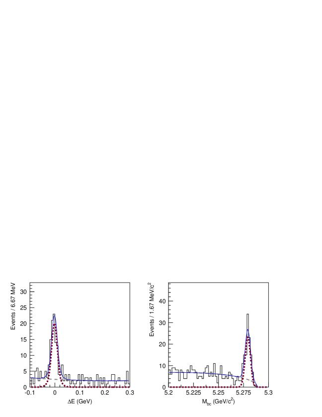
(b)
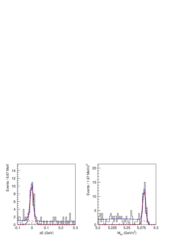
(c)

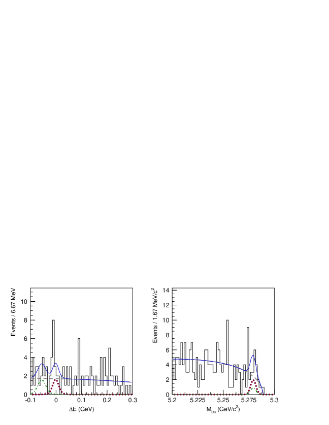
Figure 2: Distributions of ${\Delta{E}}$ (with $5.27$ GeV/c${}^{2}<{M_{\rm bc}}<5.29$ GeV/c²) and ${M_{\rm bc}}$ (with $|{\Delta{E}}|<0.05$ GeV) for (a) $B^{+}\to{\Lambda\bar{\Lambda}K^{+}}$, (b) $B^{0}\to{\Lambda\bar{\Lambda}K^{0}}$ and (c) $B^{+}\to{\Lambda\bar{\Lambda}\pi^{+}}$ modes. The dibaryon mass $M_{\Lambda\bar{\Lambda}}$ is required to be less than 2.85 GeV/c². The solid curves, dotted curves, and dashed curves represent the total fit result, fitted signal and fitted background, respectively. The dot-dashed curves in plot (c) show the background contribution from the $B^{+}\to{\Lambda\bar{\Lambda}K^{+}}$ mode.

(a)
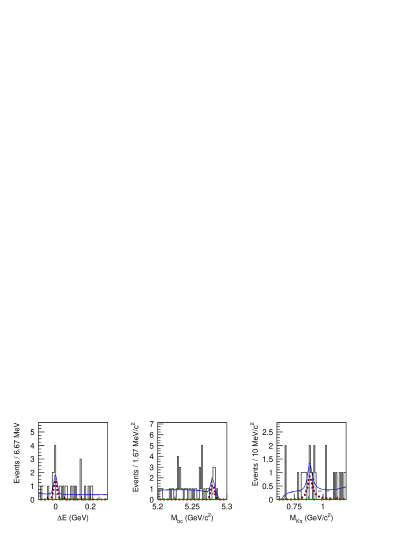
(b)

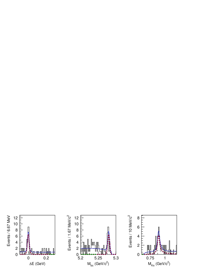
Figure 3: Distributions of ${\Delta{E}}$ (with $5.27$ GeV/c${}^{2}<{M_{\rm bc}}<5.29$ GeV/c² and $0.816<M_{K\pi}<0.976$ GeV/c²), ${M_{\rm bc}}$ (with $|{\Delta{E}}|<0.05$ GeV and $0.816$ GeV/c${}^{2}<M_{K\pi}<0.976$ GeV/c²) and $M_{K\pi}$ (with $|{\Delta{E}}|<0.05$ GeV and $5.27$ GeV/c${}^{2}<{M_{\rm bc}}<5.29$ GeV/c²) for (a) $B^{+}\to{\Lambda\bar{\Lambda}K^{*+}}$ and (b) $B^{0}\to{\Lambda\bar{\Lambda}K^{*0}}$ modes in the threshold-mass-enhanced region. The solid curves, dotted curves, and dashed curves represent the total fit result, fitted signal and fitted background, respectively.

IV Physics Results

IV.1 Fitting Results

Figures 2 and 3 show the fit results for $B^{+}\to{\Lambda\bar{\Lambda}K^{+}}$, $B^{0}\to{\Lambda\bar{\Lambda}K^{0}}$, $B^{+}\to{\Lambda\bar{\Lambda}\pi^{+}}$, $B^{+}\to{\Lambda\bar{\Lambda}K^{*+}}$ and $B^{0}\to{\Lambda\bar{\Lambda}K^{*0}}$ in the $M_{\Lambda\bar{\Lambda}}$ region below 2.85 GeV/c², which we refer to as the threshold-mass-enhanced region. The resulting signal yields are given in Table 1. The significance is defined as $\sqrt{-2{\rm ln}(L_{0}/L_{\rm max})}$, where $L_{0}$ and $L_{\rm max}$ are the likelihood values returned by the fit with the signal yield fixed to zero and at its best fit value. These values include the systematic uncertainty obtained by varying signal PDF parameters by their 1 $\sigma$ errors.

Table 1: Signal yields for each decay mode with $M_{\Lambda\bar{\Lambda}}<$ 2.85 GeV/c².

Mode	${\Lambda\bar{\Lambda}K^{+}}$	${\Lambda\bar{\Lambda}K^{0}}$	${\Lambda\bar{\Lambda}\pi^{+}}$	${\Lambda\bar{\Lambda}K^{*+}}$	${\Lambda\bar{\Lambda}K^{*0}}$
Yield	$92.7^{+11.0}_{-10.3}$	$45.8^{+7.6}_{-6.9}$	$7.76^{+4.49}_{-3.72}$	$6.54^{+3.37}_{-2.63}$	$31.4^{+7.4}_{-6.8}$
Significances ($\sigma$)	16.4	12.4	2.5	3.7	9.3

(a)                                                     (b)

(c)

Figure 4: Differential branching fractions for (a) $B^{+}\to{\Lambda\bar{\Lambda}K^{+}}$, (b) $B^{0}\to{\Lambda\bar{\Lambda}K^{0}}$ and (c) $B^{0}\to{\Lambda\bar{\Lambda}K^{*0}}$ modes as a function of $M_{\Lambda\bar{\Lambda}}$. Note that two bins with 2.850 GeV/c² $<M_{\Lambda\bar{\Lambda}}<$ 3.128 GeV/c² and 3.315 GeV/c² $<M_{\Lambda\bar{\Lambda}}<$ 3.735 GeV/c² contain charmonium events and are excluded from the charmless signal yields. The solid histograms are from phase space MC simulation with area normalized to the charmless signal yield.

Table 2: Signal yields and branching fractions ${\cal B}$ ($10^{-6}$) in different $M_{\Lambda\bar{\Lambda}}$ regions for $B^{+}\to{\Lambda\bar{\Lambda}K^{+}}$ and $B^{0}\to{\Lambda\bar{\Lambda}K^{0}}$ decays. The ${\dagger}$ symbol indicates a charm veto bin.

	$B^{+}\to{\Lambda\bar{\Lambda}K^{+}}$		$B^{0}\to{\Lambda\bar{\Lambda}K^{0}}$
$M_{\Lambda\bar{\Lambda}}$ (GeV/c2)	Yield	${\cal B}$ ($10^{-6}$)	Yield	${\cal B}$ ($10^{-6}$)
$<2.4$	$50.6^{+7.9}_{-7.2}$	$1.65^{+0.26}_{-0.23}$	$20.8^{+5.1}_{-4.4}$	$1.96^{+0.48}_{-0.41}$
$2.4-2.6$	$24.7^{+5.9}_{-5.2}$	$0.85^{+0.20}_{-0.18}$	$18.3^{+4.8}_{-4.2}$	$1.84^{+0.49}_{-0.42}$
$2.6-2.85$	$17.5^{+5.3}_{-4.6}$	$0.61^{+0.18}_{-0.16}$	$5.9^{+3.4}_{-2.7}$	$0.61^{+0.35}_{-0.28}$
$2.85-3.128$ (†)	$117.5^{+11.8}_{-11.2}$	$3.70^{+0.37}_{-0.35}$	$39.3^{+7.0}_{-6.3}$	$3.79^{+0.67}_{-0.60}$
$3.128-3.315$	$5.0^{+3.9}_{-3.1}$	$0.14^{+0.11}_{-0.09}$	$1.2^{+2.0}_{-1.2}$	$0.11^{+0.17}_{-0.10}$
$3.315-3.735$ (†)	$16.0^{+5.2}_{-4.5}$	$0.41^{+0.13}_{-0.11}$	$3.0^{+2.4}_{-1.7}$	$0.26^{+0.21}_{-0.15}$
$3.735-4.3$	$3.7^{+3.8}_{-3.0}$	$0.08^{+0.09}_{-0.07}$	$2.6^{+2.5}_{-1.8}$	$0.22^{+0.21}_{-0.15}$
$>4.3$	$1.9^{+3.3}_{-2.5}$	$0.05^{+0.08}_{-0.06}$	$0.3^{+1.8}_{-1.0}$	$0.03^{+0.18}_{-0.11}$
charmless	$103.4^{+12.9}_{-11.2}$	$3.38^{+0.41}_{-0.36}$	$49.1^{+8.6}_{-7.0}$	$4.76^{+0.84}_{-0.68}$

Table 3: Signal yields and branching fractions ${\cal B}$ ($10^{-6}$) in different $M_{\Lambda\bar{\Lambda}}$ regions for $B^{0}\to{\Lambda\bar{\Lambda}K^{*0}}$ decay. The ${\dagger}$ symbol indicates a charm veto bin.

	$B^{0}\to{\Lambda\bar{\Lambda}K^{*0}}$
$M_{\Lambda\bar{\Lambda}}$ (GeV/c2)	Yield	${\cal B}$ ($10^{-6}$)
$<2.4$	$19.6^{+6.4}_{-5.5}$	$1.76^{+0.58}_{-0.50}$
$2.4-2.6$	$9.6^{+4.5}_{-3.7}$	$0.94^{+0.44}_{-0.37}$
$2.6-2.85$	$4.6^{+2.9}_{-2.2}$	$0.48^{+0.31}_{-0.23}$
$2.85-3.128$ (†)	$43.8^{+8.3}_{-7.7}$	$4.35^{+0.83}_{-0.77}$
$3.128-3.315$	$-1.2^{+2.4}_{-1.7}$	$-0.10^{+0.20}_{-0.14}$
$3.315-3.735$ (†)	$3.5^{+3.6}_{-2.7}$	$0.29^{+0.29}_{-0.22}$
$>3.735$	$-7.2^{+3.6}_{-3.1}$	$-0.61^{+0.31}_{-0.26}$
charmless	$25.3^{+9.4}_{-7.8}$	$2.46^{+0.87}_{-0.72}$

IV.2 Observed Branching Fractions

IV.2.1 Branching Fractions

The differential branching fractions as a function of $M_{\Lambda\bar{\Lambda}}$ for the observed modes are shown in Fig. 4. Tables 2 and 3 give the yields and the corresponding branching fractions for each $M_{\Lambda\bar{\Lambda}}$ bin. The yields are obtained from (${\Delta{E}}$, ${M_{\rm bc}}$(, $M_{K\pi}$)) unbinned extended maximum likelihood fits for each bin of $M_{\Lambda\bar{\Lambda}}$. We find that a threshold enhancement is also present for $B^{0}\to{\Lambda\bar{\Lambda}K^{*0}}$ and $B^{0}\to{\Lambda\bar{\Lambda}K^{0}}$ decays. We sum the charmless partial branching fractions, where the summation excludes bins in the two charmonium regions, to obtain: ${\mathcal{B}}(B^{+}\to{\Lambda\bar{\Lambda}K^{+}})=(3.38^{+0.41}_{-0.36}\pm 0.41)\times 10^{-6}$, ${\mathcal{B}}(B^{0}\to{\Lambda\bar{\Lambda}K^{0}})=(4.76^{+0.84}_{-0.68}\pm 0.61)\times 10^{-6}$, and ${\mathcal{B}}(B^{0}\to{\Lambda\bar{\Lambda}K^{*0}})=(2.46^{+0.87}_{-0.72}\pm 0.34)\times 10^{-6}$. For the ${\Lambda\bar{\Lambda}K^{*+}}$ mode, we find $\mathcal{B}(B^{+}\to{\Lambda\bar{\Lambda}K^{*+}})=(2.19^{+1.13}_{-0.88}\pm 0.33)\times 10^{-6}$ with 3.7$\sigma$ significance in the threshold-mass-enhanced region using the yield in Table 1. The differential branching fractions are obtained by correcting the yields for the $M_{\Lambda\bar{\Lambda}}$ dependent efficiency, which is estimated from signal MC. Here, we include the efficiency correction for $\Lambda$ polarization reported in Ref. Wang ; Suzuki as our default MC does not include such an effect. The correction factors are 1.17, 1.23, 1.20, 1.22, and 1.16 for $B^{+}\to{\Lambda\bar{\Lambda}K^{+}}$, $B^{+}\to{\Lambda\bar{\Lambda}\pi^{+}}$, $B^{0}\to\Lambda\bar{\Lambda}{K^{0}}$, $B^{0}\to{\Lambda\bar{\Lambda}K^{*0}}$ and $B^{+}\to{\Lambda\bar{\Lambda}K^{*+}}$, respectively. These factors are obtained in a model independent way. We first use the phase space MC sample to obtain the efficiency function in $\cos\theta_{p}$, where $\cos\theta_{p}$ is the polar angle of proton in the $\Lambda$ helicity frame. We then use the $\cos\theta_{p}$ distributions in the data sideband and signal regions to find their corresponding average efficiencies. With the signal yield information from the fit, the model independent signal efficiency can be estimated. Fig. 5 shows the differential branching fractions in bins of $\cos\theta_{p}$ for $B^{+}\to\Lambda\bar{\Lambda}K^{+}$. This distribution is not flat but does agree with the theoretical expectation Suzuki .

Figure 5: Differential branching fractions vs. $\cos\theta_{p}$ for $B^{+}\to\Lambda\bar{\Lambda}K^{+}$ in the threshold-mass-enhanced region.

To verify the branching fraction measurement procedure, we use $J/\psi$ $K^{(*)}$ events with $J/\psi\to\Lambda\bar{\Lambda}$ in the region $3.070~{}{\rm GeV/c^{2}}<M_{\Lambda\bar{\Lambda}}<3.125~{}{\rm GeV/c^{2}}$. Using $\mathcal{B}(J/\psi\to\Lambda\bar{\Lambda})=(1.61\pm 0.15)\times 10^{-3}$ PDG , we obtain branching fractions of $(1.30^{+0.21}_{-0.20})\times 10^{-3}$, $(0.66^{+0.23}_{-0.19})\times 10^{-3}$, and $(2.08^{+0.45}_{-0.42})\times 10^{-3}$ for $B^{+}\to J/\psi K^{+}$, $B^{0}\to J/\psi K^{0}$, $B^{0}\to J/\psi K^{*0}$, respectively, which agree with the world average values PDG within $2\sigma$ including systematic errors that are similar to those for the signal mode discussed below.

IV.2.2 Polar Angle Distribution

Figure 6 shows the angular distribution of the $\bar{\Lambda}$ in the $\Lambda\bar{\Lambda}$ rest frame for the threshold-mass-enhanced region. The yields are obtained from (${\Delta{E}}$, ${M_{\rm bc}}$) unbinned extended maximum likelihood fits for each bin of $\cos\theta_{\bar{\Lambda}}$. The angle $\theta_{\bar{\Lambda}}$ is defined as the angle between the $\bar{\Lambda}$ direction and the $K^{+}$ direction in the $\Lambda\bar{\Lambda}$ pair rest frame. Here, we make a $\cos\theta_{\bar{\Lambda}}$ dependent efficiency correction and an average correction for the $\bar{\Lambda}$ helicity dependence as discussed above. The distribution shows no significant forward peak, in contrast to the prominent peak reported in $B^{+}\to{p\bar{p}K^{+}}$ polar , which is a unique signature of the intriguing result discussed above.

Figure 6: Differential branching fractions vs. $\cos\theta_{\bar{\Lambda}}$ in the $\Lambda\bar{\Lambda}$ pair system for $B^{+}\to{\Lambda\bar{\Lambda}K^{+}}$ in the threshold-mass-enhanced region.

IV.2.3 Helicity Distribution

We study the $K^{*0}$ polarization in ${\Lambda\bar{\Lambda}K^{*0}}$ decay, as the ${K^{*0}}$ meson is found to be almost 100% polarized with a fraction of $(101\pm 13\pm 3)\%$ in the helicity zero state in $B^{0}\to{p\bar{p}K^{*0}}$ decay JHChen . To study the $K^{*0}$ polarization, we use a MC simulation to obtain the efficiency as a function of $\cos\theta_{K}$ in the threshold-mass-enhanced region, where the angle $\theta_{K}$ is defined as the angle between the opposite $B$ direction and the $K^{+}$ direction in the $K^{*0}$ rest frame. We separate the $\cos\theta_{K}$ distribution into 4 bins for data. We then use (${\Delta{E}}$, ${M_{\rm bc}}$, $M_{K\pi}$) unbinned extended maximum likelihood fits to obtain signal yields in bins of $\cos\theta_{K}$ and calculate the branching fractions for each bin with the corresponding efficiency. Finally, we use $D^{1}_{00}$ and $D^{1}_{10}$ functions, i.e. $\frac{3}{2}\cos^{2}\theta_{K}$ for a pure helicity zero state and $\frac{3}{4}\sin^{2}\theta_{K}$ for a pure helicity one ($\pm 1$) state, to fit this branching fraction distribution. The fit result is shown in Fig. 7. We find that the ${K^{*0}}$ meson is polarized with $(60\pm 22\pm 8)\%$ in the helicity zero state.

Figure 7: Differential branching fractions vs. $\cos\theta_{K}$ in the $K^{*0}$ system for $B^{0}\to{\Lambda\bar{\Lambda}K^{*0}}$ in the threshold-mass-enhanced region. The solid curve is the result of the fit.

IV.2.4 Upper Limits and Interpretation

For modes with signal significance less than 4$\sigma$, we set the corresponding upper limits on the decay branching fractions at the 90% confidence level in the threshold-mass-enhanced region. Using the methods described in Refs. Gary ; Conrad , we obtain ${\mathcal{B}}(B^{+}\to{\Lambda\bar{\Lambda}K^{*+}})<4.98\times 10^{-6}$, where the systematic uncertainty has been taken into account.

Naively, one would expect that the ratio of $\mathcal{B}(B^{+}\to{\Lambda\bar{\Lambda}\pi^{+}})$ to $\mathcal{B}(B^{+}\to{\Lambda\bar{\Lambda}K^{+}})$ is similar to the one of $\mathcal{B}(B^{+}\to{p\bar{p}\pi^{+}})$ to $\mathcal{B}(B^{+}\to{p\bar{p}K^{+}})$ Wei . The anticipated signal yield for $B^{+}\to{\Lambda\bar{\Lambda}\pi^{+}}$ is $26.83^{+4.46}_{-4.13}$. However, we find no significant signal in the threshold-mass-enhanced region for $B^{+}\to{\Lambda\bar{\Lambda}\pi^{+}}$ and obtain the upper limit ${\mathcal{B}}(B^{+}\to{\Lambda\bar{\Lambda}\pi^{+}})<0.94\times 10^{-6}$ at the 90% confidence level. As a cross-check, we measure $\mathcal{B}(B^{+}\to{\Lambda\bar{\Lambda}K^{+}})=(3.57^{+1.82}_{-1.54})\times 10^{-6}$ using the misidentified $B^{+}\to{\Lambda\bar{\Lambda}K^{+}}$ component in the fit. This value agrees well with our ${\mathcal{B}}(B^{+}\to{\Lambda\bar{\Lambda}K^{+}})$ measurement.

Our results may indicate that the contribution of the $sd-\bar{s}\bar{d}$ popping diagram to $B^{+}\to{\Lambda\bar{\Lambda}\pi^{+}}$ shown in Fig. 9(b), is suppressed relative to the $ud-\bar{u}\bar{d}$ popping diagram shown in Fig. 9(a). In light of this observation, we move to the $b\to c$ tree diagram (internal W emission) dominated decay $B^{0}\to\Lambda\bar{\Lambda}\bar{D^{0}}$ ($us-\bar{u}\bar{s}$ popping), which is shown in Fig. 9(d). We select the 1.852 GeV/c${}^{2}<M_{K^{+}\pi^{-}}<$ 1.877 GeV/c² region for $\bar{D^{0}}$ candidates and extract the $B$ yield. Figure 8 shows the result of the fit. The signal yield is $5.53_{-2.35}^{+3.04}$ with a significance of 3.4$\sigma$. The branching fraction $\mathcal{B}(B^{0}\to\Lambda\bar{\Lambda}\bar{D}^{0})$ is $(1.05_{-0.44}^{+0.57})\times 10^{-5}$ $<2.60\times 10^{-5}$ at the 90% confidence level. This branching fraction contrasts with the large, $(1.14\pm 0.09)\times 10^{-4}$ PDG , branching fraction observed for $B^{0}\to{p\bar{p}}\bar{D^{0}}$ ($uu-\bar{u}\bar{u}$ popping) shown in Fig. 9(c). It appears that the diquark pair popping from the vacuum for $us-\bar{u}\bar{s}$ is considerably suppressed compared with $uu-\bar{u}\bar{u}$.

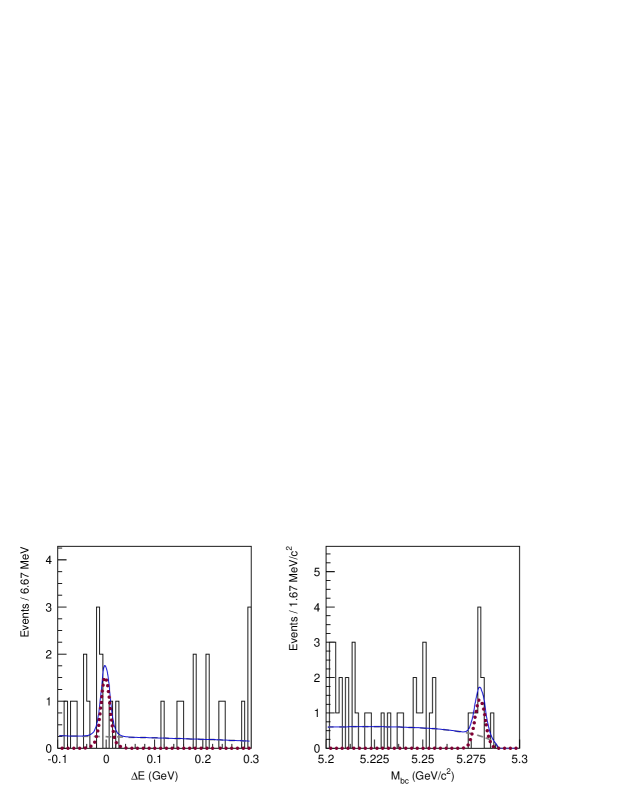
Figure 8: Distributions of ${\Delta{E}}$ (with $5.27$ GeV/c${}^{2}<{M_{\rm bc}}<5.29$ GeV/c²) and ${M_{\rm bc}}$ (with $|{\Delta{E}}|<0.05$ GeV) for the $B^{0}\to\Lambda\bar{\Lambda}\bar{D^{0}}$ mode. The result includes the whole $M_{\Lambda\bar{\Lambda}}$ region. The solid curves, dotted curves, and dashed curves show the total fit result, fitted signal and fitted background, respectively.

(a)                                                          (b)

(c)                                                          (d)

Figure 9: Possible diagrams that contribute to $B^{+}\to{p\bar{p}\pi^{+}}$/${\Lambda\bar{\Lambda}\pi^{+}}$ and $B^{0}\to{p\bar{p}}\bar{D^{0}}$/$\Lambda\bar{\Lambda}\bar{D^{0}}$.

IV.3 Comparison with predictions and previous measurements

Table 4 shows a comparison of the branching fractions for $B^{+}\to{\Lambda\bar{\Lambda}K^{+}}$, $B^{+}\to{\Lambda\bar{\Lambda}\pi^{+}}$ and $B^{0}\to{\Lambda\bar{\Lambda}K^{0}}$ decays to previous measurements YJLee and to theoretical predictions prediction , which are based on the experimental data for $B\to{p\bar{p}}h$ and $B\to p\bar{\Lambda}h$ decays.

The branching fractions of $B^{+}\to{\Lambda\bar{\Lambda}K^{+}}$ and $B^{+}\to{\Lambda\bar{\Lambda}\pi^{+}}$ seem to be consistent with the theoretical predictions and the results from previous measurements.

Table 4: Comparison of branching fractions to previous results and theoretical predictions.

Mode	Theoretical predictionprediction	Previous measurementYJLee	Results of our study
${\Lambda\bar{\Lambda}K^{+}}$	$(2.8\pm 0.2)\times 10^{-6}$	$(2.91^{+0.90}_{-0.70}\pm 0.38)\times 10^{-6}$	$(3.38^{+0.41}_{-0.36}\pm 0.41)\times 10^{-6}$
${\Lambda\bar{\Lambda}\pi^{+}}$	$(1.7\pm 0.7)\times 10^{-7}$	$<2.8\times 10^{-6}$	($<0.94\times 10^{-6}$)†
$\Lambda\bar{\Lambda}{K^{0}}$	$(2.5\pm 0.3)\times 10^{-6}$	-	$(4.76^{+0.84}_{-0.68}\pm 0.61)\times 10^{-6}$

${\dagger}$: This value is obtained in the threshold-mass-enhanced region.

IV.4 Systematic Study

Systematic uncertainties are determined using high statistics control data samples.

IV.4.1 Reconstruction Efficiency

• Tracking uncertainty:
  Tracking uncertainty is determined with fully and partially reconstructed $D^{*}$ samples. It is about 1.3% per charged track.

• Particle identification uncertainty:
  For proton identification, we use a $\Lambda\to p\pi^{-}$ sample, while for $K/\pi$ identification we use a $D^{*+}\to D^{0}\pi^{+}$, $D^{0}\to K^{-}\pi^{+}$ sample. Note that the average efficiency difference for proton identification between data and MC has been corrected to obtain the final branching fraction measurements. The corrections are 7.41%, 7.40%, 7.40%, 7.45% and 7.48% for the $B^{+}\to{\Lambda\bar{\Lambda}K^{+}}$, $B^{+}\to{\Lambda\bar{\Lambda}\pi^{+}}$, $B^{0}\to\Lambda\bar{\Lambda}{K^{0}}$, $B^{+}\to{\Lambda\bar{\Lambda}K^{*+}}$ and $B^{0}\to{\Lambda\bar{\Lambda}K^{*0}}(\bar{D^{0}})$ modes, respectively. The uncertainties associated with the particle identification corrections are estimated to be 2% for the proton(anti-proton) from $\Lambda$($\bar{\Lambda}$) and 0.8% for each kaon/pion identification.

• $\Lambda$ Reconstruction:
  We vary the $\Lambda$ selection criteria to estimate their impact on the systematic uncertainty. The uncertainties from the $\Lambda$ mass cut and requirements on kinematic variables are 1.9% and 1.5%, respectively. For the reconstruction of $\Lambda$ and $\bar{\Lambda}$, we have an additional uncertainty of 4.7% in the efficiency for displaced vertex reconstruction. This is determined from the difference between $\Lambda$ proper time distributions for data and MC simulation.

• ${K_{S}^{0}}$ Reconstruction:
  The uncertainty in ${K_{S}^{0}}$ reconstruction is determined from a large sample of $D^{-}\to{K_{S}^{0}}\pi^{-}$ events. We have an additional uncertainty of 4.9% for ${K_{S}^{0}}$ reconstruction.

• ${\mathcal{R}}$ selection:
  We study the ${\mathcal{R}}$ continuum suppression by varying the ${\mathcal{R}}$ cut value from 0 to 0.9 to check for a systematic trend.

• Multiple Candidates:
  The systematic uncertainty in the best $B$ candidate selection is determined by including multicandidate events satisfying the $\cal R$ cut value when obtaining the signal yield and the efficiency for each mode. We then take the difference in the branching fractions with and without the best candidate selection as the systematic uncertainty.

• MC statistical uncertainty:
  The MC statistical uncertainty is less than 2%.

IV.4.2 Fitting Uncertainty

• PDF uncertainty:
  A systematic uncertainty in the fit yield is determined by varying the parameters of the signal and background PDFs. The assumption of uncorrelated PDFs for ${M_{\rm bc}}$ and ${\Delta{E}}$ is studied by using 2D smoothed histogram functions for both signal and $q\bar{q}$ MC events. The percentage change in the signal yield is about 0.8%. According to our MC simulation study, the rare $B$ decays that will significantly affect our signal determination are $B^{+}\to{\Lambda\bar{\Lambda}K^{+}}$ for $B^{+}\to{\Lambda\bar{\Lambda}\pi^{+}}$ mode and $B\to\Lambda\bar{\Sigma}^{0}$h for all $B\to\Lambda\bar{\Lambda}h$ modes. The latter contributes a 0.5% error and is included in the systematic error from fitting. The uncertainty in the fit from the $M_{K\pi}$ PDF for continuum background is determined from the difference between the fit results for the $B\to{p\bar{p}}K^{*}$ modes using analytical functions (a threshold function and a p-wave function) and using the smooth function obtained from the $M_{K\pi}$ distribution in sideband data JHChen . We quote 1% fitting uncertainties for the $M_{K\pi}$ PDF of continuum background in $B\to\Lambda\bar{\Lambda}K^{*}$ modes. We quote a 3.2% fitting uncertainty for the $M_{K\pi}$ PDF of non-resonant $B\to\Lambda\bar{\Lambda}K\pi$, which is obtained from the difference in the fit results for the ${p\bar{p}}K\pi$ mode using an analytical function(the LASS function) and using a second order polynomial. The second order polynomial is $(x-M_{K\pi(\rm lowerb)})\times(x-M_{K\pi(\rm upperb)})$, where $M_{K\pi(\rm lowerb)}$ is 0.63325 GeV/$c^{2}$ and $M_{K\pi(\rm upperb)}$ is 1.8, 2.4 or 3.0 GeV/$c^{2}$. The uncertainty in the fit for the $M_{K\pi}$ PDF of non-resonant ${p\bar{p}}K\pi$ is largest (3.2%) when $M_{K\pi(\rm upperb)}$ is 1.8 GeV/$c^{2}$ JHChen . The total fitting uncertainties for $B^{+}\to{\Lambda\bar{\Lambda}K^{+}}$, $B^{+}\to{\Lambda\bar{\Lambda}\pi^{+}}$, $B^{0}\to{\Lambda\bar{\Lambda}K^{0}}$, $B^{0}\to{\Lambda\bar{\Lambda}K^{*0}}$ and $B^{+}\to{\Lambda\bar{\Lambda}K^{*+}}$ modes are 1.5%, 2.0%, 1.5%, 6.0% and 6.0%, respectively.

• Fitting bias:
  We use 800 simulated MC event sets to measure the difference between the fit result and the expected value. The bias is less than 1% for both 2D and 3D fits.

IV.4.3 MC modeling

• Angular distribution of the proton in the $\Lambda$ rest frame:
  As described in  IV.2.1, the efficiency uncertainty due to the polarization of $\Lambda$ ($\bar{\Lambda}$) is bypassed by using a model independent method based on data. However, to be conservative, we quote the percentage difference between efficiencies obtained from the model independent method and from the theoretically predicted $\cos\theta_{p}$ distribution Suzuki . This modeling uncertainty is about 4.3%.

• Angular distribution of the $\bar{\Lambda}$ in the $\Lambda\bar{\Lambda}$ rest frame:
  We choose the most significant mode, $B^{+}\to{\Lambda\bar{\Lambda}K^{+}}$, with $M_{\Lambda\bar{\Lambda}}<$ 2.85 GeV/c² to obtain its $\cos\theta_{\bar{\Lambda}}$ IV.2.2 distribution, shown in Fig. 6. Although it deviates significantly from a phase space distribution, the overall efficiency difference from a phase space MC sample is small since the efficiency versus $\cos\theta_{\bar{\Lambda}}$ is symmetric and flat. We assume that this effect is the same for all other decay modes. Thus, the uncertainties from the MC modeling for the angular distribution of $\cos\theta_{\bar{\Lambda}}$ are determined to be 0.9%.

• Angular distribution of kaon in $K^{*0}$ rest frame:
  The uncertainties from the MC modeling of the $\cos\theta_{K}$ angular distribution in the ${\Lambda\bar{\Lambda}K^{*0}}$ mode about 2.5%. This value is determined from the difference between the efficiency in the threshold-mass-enhanced region obtained from the $B$ yields using phase space MC event samples and the efficiency calculated from the efficiency distribution function, the theoretical PDFs for the $K^{*0}$ meson and the ratio of the two helicity states obtained by fitting to data.

IV.4.4 Total systematic errors

The systematic uncertainties for each decay channel are summarized in Table 5. These uncertainties are summed in quadrature to determine the total systematic uncertainty for each mode.

Table 5: Contributions to the systematic uncertainty(in %).

Source	${\Lambda\bar{\Lambda}K^{+}}$	${\Lambda\bar{\Lambda}\pi^{+}}$	$\Lambda\bar{\Lambda}{K^{0}}$	${\Lambda\bar{\Lambda}K^{*+}}$	${\Lambda\bar{\Lambda}K^{*0}}$	$\Lambda\bar{\Lambda}\bar{D^{0}}$
Tracking	6.8	6.8	7.8	9.2	7.9	7.9
Proton ID	4.0	4.0	4.0	4.0	4.0	4.0
Charged Kaon(Pion) ID	0.8	0.8	-	0.8	1.6	1.6
$\Lambda$ Reconstruction	4.7	4.7	4.7	4.7	4.7	4.7
$\Lambda$ Selection Cut	2.4	2.4	2.4	2.4	2.4	2.4
${K_{S}^{0}}$ Reconstruction	-	-	4.9	4.9	-	-
$\mathcal{R}$ Selection	5.3	5.3	1.3	3.5	3.5	3.5
Multiple Candidates	0.9	0.9	2.4	1.4	1.4	1.4
MC Statistics	1.0	1.0	1.5	2.0	2.0	2.0
PDF uncertainties	1.7	2.2	1.7	6.1	6.1	3.7
Fitting bias	1.0	1.0	1.0	1.0	1.0	1.0
MC modeling	4.4	4.4	4.4	4.4	5.1	4.4
Secondary decays PDG	1.6	1.6	1.6	1.6	1.6	2.0
Number of $B\bar{B}$ Pairs	1.4	1.4	1.4	1.4	1.4	1.4
Total	12.2	12.3	12.9	15.3	14.0	12.9

V Summary

Using 657 $\times 10^{6}B\bar{B}$ events, we observe low mass $M_{\Lambda\bar{\Lambda}}$ enhancements near threshold for both the ${\Lambda\bar{\Lambda}K^{0}}$ and ${\Lambda\bar{\Lambda}K^{*0}}$ modes, with 12.4$\sigma$ and 9.3$\sigma$ significance, respectively. We update the branching fraction of $B^{+}\to{\Lambda\bar{\Lambda}K^{+}}$ mode superseding the previous measurement YJLee , and set upper limits on the modes $B^{+}\to{\Lambda\bar{\Lambda}K^{*+}}$ and $B^{+}\to{\Lambda\bar{\Lambda}\pi^{+}}$ in the threshold-mass-enhanced region. No significant signal is found in the related mode $B^{0}\to\Lambda\bar{\Lambda}\bar{D}^{0}$. All the details are summarized in Table 6. The small value of $\mathcal{B}(B^{+}\to{\Lambda\bar{\Lambda}\pi^{+}})$, the large value of $\mathcal{B}(B^{0}\to{\Lambda\bar{\Lambda}K^{0}})$, and the absence of a peaking feature in the $\cos\theta_{\bar{\Lambda}}$ distribution for $B^{+}\to{\Lambda\bar{\Lambda}K^{+}}$ indicate that the underlying dynamics of $B\to\Lambda\bar{\Lambda}h$ are quite different from those of $B\to{p\bar{p}}h$. These results also imply that the $\bar{s}$ quark from $\bar{b}\to\bar{s}$ penguin diagram does not necessarily hadronize to form a $K^{+}$; the probability of forming a $\bar{\Lambda}$ is not negligible. In addition, because $\mathcal{B}(B^{0}\to\Lambda\bar{\Lambda}\bar{D^{0}}(B^{+}\to{\Lambda\bar{\Lambda}\pi^{+}})$) is much smaller than $\mathcal{B}(B^{0}\to{p\bar{p}}\bar{D^{0}}(B^{+}\to{p\bar{p}\pi^{+}}$)), it appears that diquark pair popping out from the vacuum for $us-\bar{u}\bar{s}$ ($sd-\bar{s}\bar{d}$) is suppressed compared to $uu-\bar{u}\bar{u}$ ($ud-\bar{u}\bar{d}$).

Table 6: Summary of all $B\to\Lambda\bar{\Lambda}h$ results.

Charmless branching fractions.
Mode	Yield	$\mathcal{B}(10^{-6})$	Significances ($\sigma$)
$B^{0}\to{\Lambda\bar{\Lambda}K^{0}}$	$49.1_{-7.1}^{+8.6}$	$4.76_{-0.68}^{+0.84}\pm 0.61$	12.5
$B^{0}\to{\Lambda\bar{\Lambda}K^{*0}}$	$25.3_{-7.8}^{+9.4}$	$2.46_{-0.72}^{+0.87}\pm 0.34$	9.0
$B^{+}\to{\Lambda\bar{\Lambda}K^{+}}$	$103.4_{-11.2}^{+12.9}$	$3.38_{-0.36}^{+0.41}\pm 0.41$	16.5
Results in the threshold-mass-enhanced region.
Mode	Yield	$\mathcal{B}(10^{-6})$	Significances ($\sigma$)
$B^{+}\to{\Lambda\bar{\Lambda}\pi^{+}}$	$7.76_{-3.72}^{+4.49}$	$<0.94$ at 90% C.L.	2.5
$B^{+}\to{\Lambda\bar{\Lambda}K^{*+}}$	$6.54_{-2.63}^{+3.37}$	$2.19_{-0.88}^{+1.13}\pm 0.33$	3.7
		( $<4.98$ at 90% C.L. )
Related search.
Mode	Yield	$\mathcal{B}(10^{-5})$	Significances ($\sigma$)
$B^{0}\to\Lambda\bar{\Lambda}\bar{D^{0}}$	$5.53_{-2.35}^{+3.04}$	$1.05_{-0.44}^{+0.57}\pm 0.14$	3.4
		( $<2.60$ at 90% C.L. )

We thank the KEKB group for the excellent operation of the accelerator, the KEK cryogenics group for the efficient operation of the solenoid, and the KEK computer group and the National Institute of Informatics for valuable computing and SINET3 network support. We acknowledge support from the Ministry of Education, Culture, Sports, Science, and Technology of Japan and the Japan Society for the Promotion of Science; the Australian Research Council and the Australian Department of Education, Science and Training; the National Natural Science Foundation of China under contract No. 10575109 and 10775142; the Department of Science and Technology of India; the BK21 program of the Ministry of Education of Korea, the CHEP src program and Basic Research program (grant No. R01-2008-000-10477-0) of the Korea Science and Engineering Foundation; the Polish State Committee for Scientific Research; the Ministry of Education and Science of the Russian Federation and the Russian Federal Agency for Atomic Energy; the Slovenian Research Agency; the Swiss National Science Foundation; the National Science Council and the Ministry of Education of Taiwan; and the U.S. Department of Energy.

References

(1)
M. E. Peskin, Nature 452, 293 (2008).
(2)
J.-T. Wei et al. (Belle Collaboration),
Phys. Lett. B 659, 80 (2008).
(3)
M.-Z. Wang et al. (Belle Collaboration),
Phys. Rev. D 76 , 052004 (2007).
(4)
M. Suzuki, J. Phys. G 34, 283 (2007).
(5)
J.H. Chen et al. (Belle Collaboration),
Phys. Rev. Lett. 100, 251801 (2008).
(6)
H.Y. Cheng and K.C. Yang, Phys. Rev. D 66, 014020 (2002).
(7) Throughout this report, inclusion of
charge conjugate mode is always implied unless otherwise stated.
(8)
Y.J. Lee et al. (Belle Collaboration),
Phys. Rev. Lett. 93, 211801 (2004).
(9) W.S. Hou and A. Soni,
Phys. Rev. Lett. 86, 4247 (2001).
(10)
C.Q. Geng, Y.K. Hsiao, Phys. Lett. B 619, 305 (2005)
(11)
S. Kurokawa and E. Kikutani, Nucl. Instr. and Meth. A 499, 1 (2003)
and other papers included in this Volume.
(12)
A. Abashian et al. (Belle Collaboration), Nucl. Instr. and Meth. A 479, 117 (2002).
(13)
K. Abe et al. (Belle Collaboration), Phys. Rev. D 65, 091103 (2002).
(14)
R. Brun et al., GEANT 3.21, CERN Report No. DD/EE/84-1, 1987.
(15)R.A. Fisher, Annals of Eugenics 7, 179 (1936).
(16)
S.H. Lee et al. (Belle Collab.), Phys. Rev. Lett. 91, 261801 (2003).
(17)
D. Aston et al. (LASS Collaboration), Nucl. Phys. B 296, 493 (1988).
(18)H. Albrecht et al. (ARGUS Collaboration),
Phys. Lett. B 241, 278 (1990); ibid. B 254, 288 (1991).
(19)
M. Suzuki, J. Phys. G 29, B15 (2003).
(20)
C. Amsler et al. (Particle Data Group), Phys. Lett. B 667, 1 (2008)
(21)
M.Z. Wang et al. (Belle Collaboration),
Phys. Lett. B 617, 141 (2005).
(22) G.J. Feldman and R.D. Cousins, Phys. Rev. D 57,
3873 (1998).
(23) J. Conrad et al.,
Phys. Rev. D 67, 012002 (2003).