On the Spectrum of a Quantum Dot
with Impurity in the Lobachevsky Plane

Abstract

A model of a quantum dot with impurity in the Lobachevsky plane is considered. Relying on explicit formulae for the Green function and the Krein $Q-$function which have been derived in a previous work we focus on the numerical analysis of the spectrum. The analysis is complicated by the fact that the basic formulae are expressed in terms of spheroidal functions with general characteristic exponents. The effect of the curvature on eigenvalues and eigenfunctions is investigated. Moreover, there is given an asymptotic expansion of eigenvalues as the curvature radius tends to infinity (the flat case limit).

1 Introduction

The influence of the hyperbolic geometry on the properties of quantum mechanical systems is a subject of continual theoretical interest for at least two decades. Numerous models have been studied so far, let us mention just few of them [1, 2, 3, 4]. Naturally, the quantum harmonic oscillator is one of the analyzed examples [5, 6]. It should be stressed, however, that the choice of an appropriate potential on the hyperbolic plane is ambiguous in this case, and several possibilities have been proposed in the literature. In [7], we have modeled a quantum dot in the Lobachevsky plane by an unbounded potential which can be interpreted, too, as a harmonic oscillator potential for this nontrivial geometry. The studied examples also comprise point interactions [8] which are frequently used to model impurities.

A Hamiltonian describing a quantum dot with impurity has been introduced in [7]. The main result of this paper is derivation of explicit formulae for the Green function and the Krein $Q-$function. The formulae are expressed in terms of spheroidal functions which are used rather rarely in the framework of mathematical physics. Further analysis is complicated by the complexity of spheroidal functions. In particular, the Green function depends on the characteristic exponent of the spheroidal functions in question rather than directly on the spectral parameter. In  fact, it seems to be possible to obtain a more detailed information on eigenvalues and eigenfunctions only by means of numerical methods. The particular case, when the Hamiltonian is restricted to the eigenspace of the angular momentum with eigenvalue 0, is worked out in [9]. In the current contribution we aim to extend the numerical analysis to the general case and to complete it with additional details.

The Hamiltonian describing a quantum dot with impurity in the Lobachevsky plane, as introduced in [7], is a selfadjoint extension of the following symmetric operator:

$$\begin{split}&\begin{split}H=-\left(\frac{\partial^{2}}{\partial\varrho^{2}}+\frac{1}{a}\coth\!\left(\frac{\varrho}{a}\right)\frac{\partial}{\partial\varrho}+\frac{1}{a^{2}}\sinh^{-2}\!\left(\frac{\varrho}{a}\right)\frac{\partial^{2}}{\partial\phi^{2}}+\frac{1}{4a^{2}}\right)+\frac{1}{4}\,a^{2}\omega^{2}\sinh^{2}\!\left(\frac{\varrho}{a}\right),\end{split}\\ &\mathop{\mathrm{missing}}{Dom}\nolimits(H)=C^{\infty}_{0}((0,\infty)\times S^{1})\subset L^{2}\!\left((0,\infty)\times S^{1},a\,\sinh(\varrho/a)\mathrm{d}\varrho\,\mathrm{d}\phi\right),\end{split}$$

where $(\varrho,\phi)$ are the geodesic polar coordinates on the Lobachevsky plane and $a$ stands for the so called curvature radius which is related to the scalar curvature by the formula $R=-2/a^{2}$. The deficiency indices of $H$ are known to be $(1,1)$ and we denote each selfadjoint extension by $H(\chi)$ where the real parameter $\chi$ appears in the boundary conditions for the domain of definition: $f(\varrho,\phi)$ belongs to $\mathop{\mathrm{missing}}{Dom}\nolimits(H(\chi))$ if there exist $f_{0},f_{1}\in\mathbb{C}$ so that $f_{1}:f_{0}=\chi:1$ and

$$f(\varrho,\phi)=-\frac{1}{2\pi}\,f_{0}\log(\varrho)+f_{1}+o(1)\textrm{~{}}\textrm{~{}as~{}}\varrho\to 0+$$

(the case $\chi=\infty$ means that $f_{0}=0$ and $f_{1}$ is arbitrary), see [7] for details. $H(\infty)$ is nothing but the Friedrichs extension of $H$. The Hamiltonian $H(\infty)$ is interpreted as corresponding to the unperturbed case and describing a quantum dot with no impurity.

After the substitution $\xi=\cosh(\varrho/a)$ and the scaling $H=a^{-2}\tilde{H}$, we make use of the rotational symmetry (which amounts to a Fourier transform in the variable $\phi$) to decompose $\tilde{H}$ into a direct sum as follows

$$\begin{split}&\tilde{H}=\bigoplus\limits_{m=-\infty}^{\infty}\tilde{H}_{m},\\ &\begin{split}\tilde{H}_{m}&=-\frac{\partial}{\partial\xi}\,(\xi^{2}-1)\,\frac{\partial}{\partial\xi}+\frac{m^{2}}{\xi^{2}-1}+\frac{a^{4}\omega^{2}}{4}\,(\xi^{2}-1)-\frac{1}{4}\,,\end{split}\\ &\mathop{\mathrm{missing}}{Dom}\nolimits(\tilde{H}_{m})=C^{\infty}_{0}(1,\infty)\subset L^{2}((1,\infty),\mathrm{d}\xi).\end{split}$$

Let us denote by $H_{m}$, $m\in\mathbb{Z}$, the restriction of $H(\infty)$ to the eigenspace of the angular momentum with eigenvalue $m$. This means that $H_{m}$ is a self-adjoint extension of $a^{-2}\tilde{H}_{m}$. It is known (Proposition 2.1 in [7]) that $\tilde{H}_{m}$ is essentially selfadjoint for $m\neq 0$. Thus, in this case, $H_{m}$ is the closure of $a^{-2}\tilde{H}_{m}$. Concerning the case $m=0$, $H_{0}$ is the Friedrichs extension of $a^{-2}\tilde{H}_{0}$. For quite general reasons, the spectrum of $H_{m}$, for any $m$, is semibounded below, discrete and simple [10]. We denote the eigenvalues of $H_{m}$ in ascending order by $E_{n,m}(a^{2})$, $n\in\mathbb{N}_{0}$.

The spectrum of the total Hamiltonian $H(\chi)$, $\chi\neq\infty$, consists of two parts (in a full analogy with the Euclidean case [11]):

1. The first part is formed by those eigenvalues of $H(\chi)$ which belong, at the same time, to the spectrum of $H(\infty)$. More precisely, this part is exactly the union of eigenvalues of $H_{m}$ for $m$ running over $\mathbb{Z}\setminus\{0\}$. Their multiplicities are discussed below in Section 5.

2. The second part is formed by solutions to the equation

   $$Q^{H}(z)=\chi$$ (1.1)

   with respect to the variable $z$ where $Q^{H}$ stands for the Krein $Q$-function of $H(\infty)$. Let us denote the solutions in ascending order by $\epsilon_{n}(a^{2},\chi)$, $n\in\mathbb{N}_{0}$. These eigenvalues are sometimes called the point levels and their multiplicities are at least one. In more detail, $\epsilon_{n}(a^{2},\chi)$ is a simple eigenvalue of $H(\chi)$ if it does not lie in the spectrum of $H(\infty)$, and this happens if and only if $\epsilon_{n}(a^{2},\chi)$ does not coincide with any eigenvalue $E_{\ell,m}(a^{2})$ for $\ell\in\mathbb{N}_{0}$ and $m\in\mathbb{Z}$, $m\neq 0$.

Remark.

The lowest point level, $\epsilon_{0}(a^{2},\chi)$, lies below the lowest eigenvalue of $H(\infty)$ which is $E_{0,0}(a^{2})$, and the point levels with higher indices satisfy the inequalities $E_{n-1,0}(a^{2})<\epsilon_{n}(a^{2},\chi)<E_{n,0}(a^{2})$, $n=1,2,3,\ldots$.

2 Spectrum of the unperturbed Hamiltonian $H(\infty)$

Our goal is to find the eigenvalues of the $m$th partial Hamiltonian $H_{m}$, i.e., to find square integrable solutions of the equation

$$H_{m}\psi(\xi)=z\psi(\xi),$$

or, equivalently,

$$\tilde{H}_{m}\psi(\xi)=a^{2}z\psi(\xi).$$

This equation coincides with the equation of the spheroidal functions (A.1) provided we set $\mu=|m|$, $\theta=-a^{4}\omega^{2}/16$, and the characteristic exponent $\nu$ is chosen so that

$$\lambda^{m}_{\nu}\!\left(-\frac{a^{4}\omega^{2}}{16}\right)=-a^{2}z-\frac{1}{4}\,.$$

The only solution (up to a multiplicative constant) that is square integrable near infinity is $S^{|m|(3)}_{\nu}(\xi,-a^{4}\omega^{2}/16)$.

Proposition A.3 describes the asymptotic expansion of this function at $\xi=1$ for $m\in\mathbb{N}$. It follows that the condition on the square integrability is equivalent to the equality

$$\mathrm{e}^{i(3\nu+1/2)\pi}K^{m}_{-\nu-1}\!\left(-\frac{a^{4}\omega^{2}}{16}\right)+K^{m}_{\nu}\!\left(-\frac{a^{4}\omega^{2}}{16}\right)=0.$$ (2.1)

Furthermore, in [7] we have derived that

$$S^{0(3)}_{\nu}(\xi,\theta)=\alpha\log(\xi-1)+\beta+O((\xi-1)\log(\xi-1))\quad\text{as }\xi\to 1+,$$

where

$$\alpha=\frac{i\tan(\nu\pi)\,\mathrm{e}^{-i(2\nu+1/2)\pi}}{2\pi s^{0}_{\nu}(\theta)}\left(\mathrm{e}^{i(3\nu+1/2)\pi}K^{0}_{-\nu-1}(\theta)+K^{0}_{\nu}(\theta)\right).$$

Taking into account that the Friedrichs extension has continuous eigenfunctions we conclude that equation (2.1) guarantees square integrability in the case $m=0$, too.

Figure 1: Eigenvalues of the partial Hamiltonian $H_{1}$

As far as we see it, equation (2.1) can be solved only by means of numerical methods. For this purpose we made use of the computer algebra system Mathematica 6.0. For the numerical computations we set $\omega=1$. The particular case $m=0$ has been examined in [9]. It turns out that an analogous procedure can be also applied for nonzero values of the angular momentum. As an illustration, Figure 1 depicts several first eigenvalues of the Hamiltonian $H_{1}$ as functions of the curvature radius $a$. The dashed asymptotic lines correspond to the flat limit ($a\to\infty$).

Denote the $n$th normalized eigenfunction of the $m$th partial Hamiltonian $\tilde{H}_{m}$ by $\tilde{\psi}_{n,m}(\xi)$. Obviously, the eigenfunctions for the values of the angular momentum $m$ and $-m$ are the same and are proportional to $S^{|m|(3)}_{\nu}(\xi,-a^{4}\omega^{2}/16)$, with $\nu$ satisfying equation (2.1). Let us return to the original radial variable $\varrho$ and, moreover, regard $\tilde{H}_{m}$ as an operator acting on $L^{2}(\mathbb{R}^{+},\mathrm{d}\varrho)$. This amounts to an obvious isometry

$$L^{2}(\mathbb{R}^{+},a^{-1}\sinh(\varrho/a)\mathrm{d}\varrho)\to{}L^{2}(\mathbb{R}^{+},\mathrm{d}\varrho):\ f(\varrho)\mapsto{}a^{-1/2}\sinh^{1/2}(\varrho/a)f(\varrho).$$

The corresponding normalized eigenfunction of $\tilde{H}_{m}$, with an eigenvalue $a^{2}z$, equals

$$\psi_{n,m}(\varrho)=\left(\frac{1}{a}\sinh\left(\frac{\varrho}{a}\right)\right)^{\!1/2}\tilde{\psi}_{n,m}\!\left(\cosh\left(\frac{\varrho}{a}\right)\right).$$ (2.2)

At the same time, relation (2.2) gives the normalized eigenfunction of $H_{m}$ (considered on $L^{2}(\mathbb{R}^{+},\mathrm{d}\varrho)$) with the eigenvalue $z$. The same Hilbert space may be used also in the limit Euclidean case ($a=\infty$). The eigenfunctions $\Phi_{n,m}$ in the flat case are well known and satisfy

$$\Phi_{n,m}\propto\varrho^{|m|+1/2}\mathrm{e}^{-\omega\varrho^{2}/4}\,{{}_{1}F_{1}}\!\left(-n,|m|+1,\frac{\omega\varrho^{2}}{2}\right).$$ (2.3)

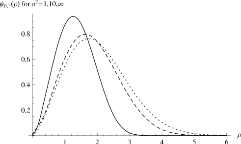
Figure 2: The first eigenfunction of the partial Hamiltonian $H_{1}$

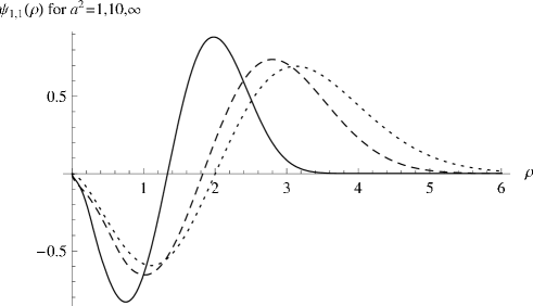
Figure 3: The second eigenfunction of the partial Hamiltonian $H_{1}$

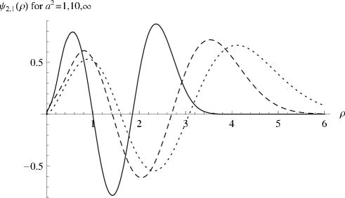
Figure 4: The third eigenfunction of the partial Hamiltonian $H_{1}$

The fact that we stick to the same Hilbert space in all cases facilitates the comparison of eigenfunctions for various values of the curvature radius $a$. We present plots of several first eigenfunctions of $H_{1}$ (Figures 2, 3, 4) for the values of the curvature radius $a=1$ (the solid line), $10$ (the dashed line), and $\infty$ (the dotted line). Again, see [9] for analogous plots in the case of the Hamiltonian $H_{0}$. Note that, in general, the smaller is the curvature radius $a$ the more localized is the particle in the region near the origin.

3 The point levels

As has been stated, the point levels are solutions to equation (1.1) with respect to the spectral parameter $z$. Since, in general, $Q(\bar{z})=\overline{Q(z)}$ the function $Q(z)$ takes real values on the real axis. Let $\tilde{H}(\infty)=a^{2}H(\infty)$ be the Friedrichs extension of $\tilde{H}$. An explicit formula for the Krein $Q$-function $Q^{\tilde{H}}(z)$ of $\tilde{H}(\infty)$ has been derived in [7]:

$$\begin{split}Q^{\tilde{H}}(z)=&-\frac{1}{4\pi a^{2}}\left(-\log(2)-2\Psi(1)+2\,\Psi s_{\nu}\!\left(-\frac{a^{4}\omega^{2}}{16}\right)s^{0}_{\nu}\!\left(-\frac{a^{4}\omega^{2}}{16}\right)\right)\\ &+\frac{1}{2a^{2}\tan(\nu\pi)}\left(\mathrm{e}^{i\pi(3\nu+3/2)}\,\frac{K^{0}_{-\nu-1}(-\frac{a^{4}\omega^{2}}{16})}{K^{0}_{\nu}(-\frac{a^{4}\omega^{2}}{16})}-1\right)^{\!-1}+\frac{\log{(2a^{2})}}{4\pi a^{2}},\end{split}$$

where $\nu$ is chosen so that

$$\lambda^{0}_{\nu}\!\left(-\frac{a^{4}\omega^{2}}{16}\right)=-z-\frac{1}{4}\,.$$

The symbol $K^{0}_{\nu}(\theta)$ stands for the so called spheroidal joining factor,

$$\Psi{}s_{\nu}(\theta):=\sum^{\infty}_{r=-\infty}(-1)^{r}a^{0}_{\nu,r}(\theta)\,\Psi(\nu+1+2r),$$

where the coefficients $a^{0}_{\nu,r}(\theta)$, $r\in\mathbb{Z}$, come from the expansion of spheroidal functions in terms of Bessel functions (for details see [7, the Appendix])), and $s^{0}_{\nu}(\theta)$ is defined by formula (A.4). One can obtain the Krein $Q$-function of $H(\infty)$ simply by scaling $Q^{H}(z)=a^{2}\,Q^{\tilde{H}}(a^{2}z)$.

Figure 5: The Krein $Q$-function $Q^{H}$ for $a^{2}=0.02,~{}0.2,~{}1,~{}5$

Since we know the explicit expression for the Krein $Q$-function as a function of the characteristic exponent $\nu$ rather than of the spectral parameter $z$ itself it is of importance to know for which values of $\nu$ the spectral parameter $z$ is real. Propositions A.1 and A.2 give the answer. For $\nu\in\mathbb{R}$ and for $\nu$ of the form $\nu=-1/2+it$ where $t$ is real, the spheroidal eigenvalue $\lambda^{m}_{\nu}(-a^{4}\omega^{2}/16)$ is real, and so the same is true for $z$. Moreover, these values of $\nu$ reproduce the whole real $z$ axis. With this knowledge, one can plot the Krein $Q$-function $Q^{H}=Q^{H}(z)$ for an arbitrary value of the curvature radius $a$. Note that for $a=\infty$, the Krein $Q$-function is well known as a function of the spectral parameter $z$ [12] and equals (setting $\omega=1$, $\Psi$ is the logarithmic derivative of the gamma function)

$$Q(z)=\frac{1}{4\pi}\left(-\Psi\!\left(\frac{1-z}{2}\right)+\log(2)+2\Psi(1)\right).$$

Next, in Figure 5, we present plots of the Krein $Q$-function for several distinct values of the curvature radius $a$. Moreover, in Figure 6 one can compare the behavior of the Krein $Q$-function for a comparatively large value of the curvature radius ($a^{2}=24$) and for the Euclidean case ($a=\infty$).

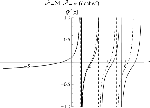
Figure 6: Comparison of the Krein $Q$-functions for $a^{2}=24$ and $a^{2}=\infty$

Again, equation (1.1) can be solved only numerically. Fixing the parameter $\chi$ one may be interested in the behavior of the point levels as functions of the curvature radius $a$. See Figure 7 for the corresponding plots, with $\chi=0$, where the dashed asymptotic lines again correspond to the flat case limit ($a=\infty$). Note that for the curvature radius $a$ large enough, the lowest eigenvalue is negative provided $\chi$ is chosen smaller than $Q(0)\simeq 0.1195$.

Figure 7: Point levels for H(0)

4 Asymptotic behavior for large values of $a$

The $m$th partial Hamiltonian $H_{m}$, if considered on $L^{2}(\mathbb{R}^{+},\mathrm{d}\varrho)$, acts like

$$H_{m}=-\frac{\partial^{2}}{\partial\varrho^{2}}+\frac{m^{2}-\frac{1}{4}}{a^{2}\sinh^{2}(\frac{\varrho}{a})}+\frac{1}{4}\,a^{2}\omega^{2}\sinh^{2}\!\left(\frac{\varrho}{a}\right)=:-\frac{\partial^{2}}{\partial\varrho^{2}}+V_{m}(a,\varrho).$$

For a fixed $\varrho\neq 0$, one can easily derive that

$$V_{m}(a,\varrho)=\frac{m^{2}-\frac{1}{4}}{\varrho^{2}}+\frac{1}{4}\omega^{2}\varrho^{2}+\frac{\frac{1}{4}-m^{2}}{3a^{2}}+\frac{\omega^{2}\varrho^{4}}{12a^{2}}+O\!\left(\frac{1}{a^{4}}\right)\quad\textrm{as~{}}a\to\infty.$$

Recall that the $m$th partial Hamiltonian of the isotropic harmonic oscillator on the Euclidean plane, $H_{m}^{E}$, if considered on $L^{2}(\mathbb{R}^{+},\mathrm{d}\varrho)$, has the form

$$H_{m}^{E}:=-\frac{\partial^{2}}{\partial\varrho^{2}}+\frac{m^{2}-\frac{1}{4}}{\varrho^{2}}+\frac{1}{4}\omega^{2}\varrho^{2}.$$

This suggests that it may be useful to view the Hamiltonian $H_{m}$, for large values of the curvature radius $a$, as a perturbation of $H_{m}^{E}$,

$$H_{m}\sim H_{m}^{E}+\frac{1}{12a^{2}}(1-4m^{2}+\omega^{2}\varrho^{4})=:H_{m}^{E}+\frac{1}{12a^{2}}U_{m}(\varrho).$$

The eigenvalues of the compared Hamiltonians have the same asymptotic expansions up to the order $1/a^{2}$ as $a\to\infty$.

Let us denote the $n$th eigenvalue of the Hamiltonian $H^{E}_{m}$ by $E^{E}_{n,m}$, $n\in\mathbb{N}_{0}$. It is well known that

$$E^{E}_{n,m}=(2n+|m|+1)\,\omega$$

and that the multiplicity of $E^{E}_{n,m}$ in the spectrum of $H^{E}$ equals $2n+|m|+1$. The asymptotic behavior of $E_{n,m}(a^{2})$ may be deduced from the standard perturbation theory and is given by the formula

$$E_{n,m}(a^{2})=E_{n,m}^{E}+\frac{1}{12a^{2}}\frac{\langle\Phi_{n,m},U_{m}\Phi_{n,m}\rangle}{\langle\Phi_{n,m},\Phi_{n,m}\rangle}+O\!\left(\frac{1}{a^{4}}\right)\quad\textrm{as~{}}a\to\infty,$$ (4.1)

where $\Phi_{n,m}$ denotes a (not necessarily normalized) eigenfunction of $H^{E}_{m}$ associated with the eigenvalue $E^{E}_{n,m}$ (see (2.3)). The scalar products occurring in formula (4.1) can be readily evaluated in $L^{2}(\mathbb{R}^{+},\mathrm{d}\varrho)$ with the help of Proposition A.4. The resulting formula takes the form

$$E_{n,m}(a^{2})=(2n+|m|+1)\,\omega+\left(2n(n+|m|+1)+|m|+\frac{3}{4}\right)\!\frac{1}{a^{2}}+O\!\left(\frac{1}{a^{4}}\right)$$ (4.2)

as $a\to\infty$. This asymptotic approximation of eigenvalues has been tested numerically for large values of the curvature radius $a$. The asymptotic eigenvalues for $a^{2}=24$ are compared with the precise numerical results in Table 1. It is of interest to note that the asymptotic coefficient in front of the $a^{-2}$ term does not depend on the frequency $\omega$.

Table 1: Comparison of numerical and asymptotic results for the eigenvalues, $a^{2}=24$

	$E_{0,0}$	$E_{1,0}$	$E_{2,0}$	$E_{0,1}$	$E_{1,1}$	$E_{2,1}$
numerical	1.0265	3.162	5.42	2.060	4.259	6.58
asymptotic	1.0268	3.169	5.46	2.058	4.258	6.59
error (%)	-0.03	-0.22	-0.74	0.10	0.02	-0.15

5 The multiplicities

Since $H_{-m}=H_{m}$ the eigenvalues $E_{n,m}(a^{2})$ of the total Hamiltonian $H(\infty)$ are at least twice degenerated if $m\neq 0$. From the asymptotic expansion (4.2) it follows, after some straightforward algebra, that no additional degeneracy occurs and thus theses eigenvalues are exactly twice degenerated at least for sufficiently large values of $a$.

Applying the methods developed in [11] one may complete the analysis of the spectrum of the total Hamiltonian $H(\chi)$ for $\chi\neq\infty$. Namely, the spectrum of $H(\chi)$ contains eigenvalues $E_{n,m}(a^{2})$, $m>0$, with multiplicity 2 if $Q^{H}(E_{n,m}(a^{2}))\neq\chi$, and with multiplicity 3 if $Q^{H}(E_{n,m}(a^{2}))=\chi$. The rest of the spectrum of $H(\chi)$ is formed by those solutions to equation (1.1) which do not belong to the spectrum of $H(\infty)$. The multiplicity of all these eigenvalues in the spectrum of $H(\chi)$ equals  1.

Appendix: Auxiliary results

In this appendix we summarize several auxiliary results. Firstly, for our purposes we need the following observations concerning spheroidal functions. The spheroidal functions are solutions to the equation

$$(1-\xi^{2})\frac{\partial^{2}\psi}{\partial\xi^{2}}-2\xi\frac{\partial\psi}{\partial\xi}+\left[\lambda^{\mu}_{\nu}(\theta)+4\theta(1-\xi^{2})-\mu^{2}(1-\xi^{2})^{-1}\right]\psi=0.$$ (A.1)

For the notation and properties of spheroidal functions see [13]. A detailed information on this subject can be found in [14], but be aware of somewhat different notation. A very brief overview of spheroidal functions is also given in the Appendix of [7].

In the last named source, the following proposition has been proved in the particular case $m=0$. But, as one can verify by a direct inspection, the proof applies to the general case $m\in\mathbb{Z}$ as well.

Proposition A.1.

Let $\nu,\theta\in\mathbb{R}$, $m\in\mathbb{Z}$. Then $\lambda^{m}_{\nu}(\theta)\in\mathbb{R}$.

The following claim is also of interest.

Proposition A.2.

Let $\nu=-1/2+it$ where $t\in\mathbb{R}$, and $\theta\in\mathbb{R}$, $m\in\mathbb{Z}$. Then $\lambda^{m}_{\nu}(\theta)\in\mathbb{R}$.

Proof.

Let us recall that the coefficients $a^{m}_{\nu,r}(\theta)$ in the series expansion of spheroidal functions in terms of Bessel functions satisfy a three term recurrence relation (see [7, the Appendix]),

$$\beta^{m}_{\nu,r}(\theta)a^{m}_{\nu,r-1}(\theta)+\alpha^{m}_{\nu,r}(\theta)a^{m}_{\nu,r}(\theta)+\gamma^{m}_{\nu,r}(\theta)a^{\mu}_{\nu,r+1}(\theta)=\lambda^{m}_{\nu}(\theta)a^{m}_{\nu,r}(\theta).$$ (A.2)

One may view the set of equations (A.2), with $r\in\mathbb{Z}$, as an eigenvalue equation for $\lambda^{m}_{\nu}(\theta)$ that is an analytic function of $\theta$. A particular solution is fixed by the condition $\lambda^{m}_{\nu}(0)=\nu(\nu+1)$. Consider the set of complex conjugated equations. Since $\overline{\beta^{m}_{\nu,r}}=\beta^{m}_{\overline{\nu},r}(\theta)=\beta^{m}_{-\nu-1,r}(\theta)$, and the similar is true for $\alpha^{m}_{\nu,r}(\theta)$ and $\gamma^{m}_{\nu,r}(\theta)$, it holds true that

$$\beta^{m}_{-\nu-1,r}(\theta)\overline{a^{m}_{\nu,r-1}(\theta)}+\alpha^{m}_{-\nu-1,r}\overline{a^{m}_{\nu,r}(\theta)}+\gamma^{m}_{-\nu-1,r}(\theta)\overline{a^{\mu}_{\nu,r+1}(\theta)}=\overline{\lambda^{m}_{\nu}(\theta)}\,\overline{a^{m}_{\nu,r}(\theta)}.$$

Since for each $\nu$ of the considered form,

$$\lambda^{m}_{-\nu-1}(0)=(-\nu-1)(-\nu)=\nu(\nu+1)=\overline{\nu(\nu+1)}=\overline{\lambda^{m}_{\nu}(0)},$$

one has $\lambda^{m}_{-\nu-1}(\theta)=\overline{\lambda^{m}_{\nu}(\theta)}$. Moreover, $\lambda^{m}_{-\nu-1}(\theta)=\lambda^{m}_{\nu}(\theta)$ in general. We conclude that $\lambda^{m}_{\nu}(\theta)\in\mathbb{R}$. ∎

Another auxiliary result concerns the asymptotic expansion of the radial spheroidal function of the third kind.

Proposition A.3.

Let $\nu\notin\left\{-1/2+k|\ k\in\mathbb{Z}\right\},\ m\in\mathbb{N}$. Then

$$\hskip-20.00003ptS^{m(3)}_{\nu}(\xi,\theta)\sim\frac{(-1)^{m}2^{m/2-1}\Gamma(m)\tan(\nu\pi)}{\pi s^{m}_{\nu}(\theta)\,\mathrm{e}^{-i(\nu+3/2)\pi}}\left(K^{m}_{-\nu-1}(\theta)+\frac{K^{m}_{\nu}(\theta)}{\mathrm{e}^{i(3\nu+1/2)\pi}}\right)\!(\xi-1)^{-m/2}$$

$$\hskip-20.00003pt\textrm{as~{}}\xi\to 1+.$$ (A.3)

Proof.

By the definition of the radial spheroidal function of the third kind,

$$S^{m(3)}_{\nu}(\xi,\theta):=\frac{1}{i\cos(\nu\pi)}\left(S^{m(1)}_{-\nu-1}(\xi,\theta)+i\mathrm{e}^{-i\nu\pi}S^{m(1)}_{\nu}(\xi,\theta)\right),$$

and by the relation between the radial and the angular spheroidal functions,

$$S^{m(1)}_{\nu}(\xi,\theta)=-\frac{\sin(\nu\pi)}{\pi}\,\mathrm{e}^{-i\nu\pi}K^{m}_{\nu}(\theta)\,Qs^{m}_{-\nu-1}(\xi,\theta),$$

one has

$$S^{m(3)}_{\nu}(\xi,\theta)=\frac{i\tan(\nu\pi)}{\pi\mathrm{e}^{-i(\nu+1)\pi}}\left(K^{m}_{-\nu-1}(\theta)Qs^{m}_{\nu}(\xi,\theta)+\frac{K^{m}_{\nu}(\theta)Qs^{m}_{-\nu-1}(\xi,\theta)}{\mathrm{e}^{i(3\nu+1/2)\pi}}\right).$$

Using the definition

$$Qs^{m}_{\nu}(\xi,\theta)=\sum_{r=-\infty}^{\infty}(-1)^{r}a^{m}_{\nu,r}(\theta)Q^{m}_{\nu+2r}(\xi)$$

and due to the well known asymptotic expansion for the Legendre functions [13],

$$Q^{m}_{\nu}(\xi)\sim(-1)^{m}2^{m/2-1}\Gamma(m)(\xi-1)^{-m/2}\quad\textrm{as~{}}\xi\to 1+\,,$$

one derives that

$$Qs^{m}_{\nu}(\xi,\theta)\sim\frac{(-1)^{m}2^{m/2-1}\Gamma(m)}{(\xi-1)^{m/2}s^{m}_{\nu}(\theta)}\quad\textrm{as~{}}\xi\to 1+,$$

where

$$(s^{m}_{\nu}(\theta))^{-1}:=\sum_{r=-\infty}^{\infty}(-1)^{r}a^{m}_{\nu,r}(\theta)=\sum_{r=-\infty}^{\infty}(-1)^{r}a^{m}_{-\nu-1,-r}(\theta)=(s^{m}_{-\nu-1}(\theta))^{-1}.$$ (A.4)

Hence $Qs^{m}_{-\nu-1}(\xi,\theta)\sim{}Qs^{m}_{\nu}(\xi,\theta)$ as $\xi\to 1+$, and one immediately obtains (A.3). ∎

Further some auxiliary computations follow that we need for evaluation of scalar products of eigenfunctions (see (4.1)).

Proposition A.4.

Let ${{}_{1}F_{1}}(a,b,t)$ stand for the Kummer confluent hypergeometric function, and $n,m,l\in\mathbb{N}_{0}$. Then

$$\begin{split}&\int_{0}^{\infty}t^{m+l}\mathrm{e}^{-t}{{}_{1}F_{1}}(-n,1+m,t)^{2}\,\mathrm{d}t\\ &=\,(m!)^{2}\sum_{k=\max\left\{0,n-l\right\}}^{n}(-1)^{n+k}{n\choose k}\frac{(k+l)!}{(k+m)!}{k+m+l\choose n+m}.\end{split}$$ (A.5)

Proof.

By definition,

$${{}_{1}F_{1}}(-n,1+m,t):=\sum^{n}_{k=0}\frac{(-n)_{k}\,t^{k}}{(1+m)_{k}\,k!}=m!\sum_{k=0}^{n}(-1)^{k}{n\choose k}\frac{t^{k}}{(m+k)!}\,.$$

Let us denote the LHS of (A.5) by $I$. Then the integral representation of the gamma function implies

$$I=(m!)^{2}\sum_{j,k=0}^{n}(-1)^{j+k}{n\choose j}{n\choose k}\frac{(j+k+m+l)!}{(m+j)!(m+k)!}\,.$$ (A.6)

Partial summation in (A.6) can be carried out,

$$\sum_{j=0}^{n}(-1)^{j}{n\choose j}\frac{(j+k+m+l)!}{(m+j)!}=\frac{\mathrm{d}^{k+l}}{\mathrm{d}x^{k+l}}\left(x^{k+m+l}(1-x)^{n}\right)\Big{|}_{x=1}.$$ (A.7)

Expression (A.7) vanishes for $k<n-l$ and equals

$$(-1)^{n}(k+l)!{k+m+l\choose n+m}$$

for $k\geq{}n-l$. The proposition follows immediately. ∎

Corollary A.5.

In the case $l=0$, (A.5) takes a particularly simple form:

$$\int_{0}^{\infty}t^{m}\mathrm{e}^{-t}{{}_{1}F_{1}}(-n,1+m,t)^{2}\,\mathrm{d}t=\frac{n!}{(m+n)!}\,.$$

References

• [1] A. Comtet, On the Landau Levels on the Hyperbolic Plane, Ann. Physics 173 (1987), 185-209.
• [2] M. Antoine, A. Comtet, and S. Ouvry, Scattering on a Hyperbolic Torus in a Constant Magnetic Field, J. Phys. A: Math. Gen. 23 (1990), 3699-3710.
• [3] Yu. A. Kuperin, R. V. Romanov, and H. E. Rudin, Scattering on the Hyperbolic Plane in the Aharonov-Bohm Gauge Field, Lett. Math. Phys. 31 (1994), 271-278.
• [4] O. Lisovyy, Aharonov-Bohm Effect on the Poincaré Disk, J. Math. Phys. 48 (2007), 052112.
• [5] D. V. Bulaev, V. A. Geyler, and V. A. Margulis, Effect of Surface Curvature on Magnetic Moment and Persistent Currents in the Two-Dimensional Quantum Ring and Dots, Phys. Rev. B 69 (2004), 195313.
• [6] J. F. Cariñena, M. F. Rañada, and M. Santander, The Quantum Harmonic Oscillator on the Sphere and the Hyperbolic Plane, Ann. Physics 322 (2007), 2249-2278.
• [7] V. Geyler, P. Šťovíček, and M. Tušek, A Quantum Dot with Impurity in the Lobachevsky Plane, in Proceedings of the 6th Workshop on Operator Theory in Krein Spaces, Birkhäuser, 2008 (to appear); arXiv:0709.2790v3 (2007).
• [8] J. Brüning and V. Geyler, Gauge-Periodic Point Perturbations on the Lobachevsky Plane, Theor. Math. Phys. 119 (1999), 687-697.
• [9] P. Šťovíček and M. Tušek, On the Harmonic Oscillator on the Lobachevsky Plane, Russian J. Math. Phys. 14 (2007), 493-497.
• [10] J. Weidmann, Linear Operators in Hilbert Spaces. Springer, 1980.
• [11] J. Brüning, V. Geyler, and I. Lobanov, Spectral Properties of a Short-Range Impurity in a Quantum Dot, J. Math. Phys. 46 (2004), 1267-1290.
• [12] V. Geyler and I. Popov, Eigenvalues Imbedded in the Band Spectrum for a Periodic Array of Quantum Dots, Rep. Math. Phys. 39 (1997), 275-281.
• [13] H. Bateman and A. Erdélyi, Higher Transcendental Functions III. McGraw-Hill Book Company, 1955.
• [14] J. Meixner and F.V. Schäfke, Mathieusche Funktionen und Sphäroidfunktionen. Springer-Verlag, 1954.
Acknowledgments
The authors wish to acknowledge gratefully partial support of the Ministry of Education of Czech Republic under the research plan MSM6840770039 (P.Š.) and from the grant No. LC06002 (M.T.).