Dynamics of Black Hole Pairs II:Spherical Orbits and the Homoclinic Limit of Zoom-Whirliness

Abstract

Spinning black hole pairs exhibit a range of complicated dynamical behaviors. An interest in eccentric and zoom-whirl orbits has ironically inspired the focus of this paper: the constant radius orbits. When black hole spins are misaligned, the constant radius orbits are not circles but rather lie on the surface of a sphere and have acquired the name “spherical orbits”. The spherical orbits are significant as they energetically frame the distribution of all orbits. In addition, each unstable spherical orbit is asymptotically approached by an orbit that whirls an infinite number of times, known as a homoclinic orbit. A homoclinic trajectory is an infinite whirl limit of the zoom-whirl spectrum and has a further significance as the separatrix between inspiral and plunge for eccentric orbits. We work in the context of two spinning black holes of comparable mass as described in the 3PN Hamiltonian with spin-orbit coupling included. As such, the results could provide a testing ground of the accuracy of the PN expansion. Further, the spherical orbits could provide useful initial data for numerical relativity. Finally, we comment that the spinning black hole pairs should give way to chaos around the homoclinic orbit when spin-spin coupling is incorporated.

A complete knowledge of the dynamics of black hole pairs is essential for future gravitational wave experiments. Yet the importance of dynamics has not always been appreciated. Although stellar mass black hole pairs are significant candidates for a first direct detection with LIGO, their detectable gravitational radiation would be emitted from nearly circular orbits – at least that was the refrain. This preferential focus on quasi-circular inspiral was motivated by considerations of long-lived binaries that begin with a modest eccentricity that is gradually shed as angular momentum is lost to gravitational waves. A fair assessment of known astrophysics, the claim discouraged analyses of orbital dynamics in favor of the simpler analysis of circular orbits.

However, black hole binaries formed by tidal capture in dense star clusters, such as globular clusters, do not conform to this story portegies-zwart1999 . As one black hole scatters with another black hole in a dense region, a burst of radiation is emitted on close encounter. Some subset of these encounters will leave the pair bound in a highly eccentric orbit that merges too quickly to circularize. Estimates conclude that as many as 30% of multi-black hole systems will retain eccentricities $>0.1$ as their waves sweep into the LIGO bandwidth wen2003 .

Most recently, a new source of eccentric mergers was predicted to have a substantial detection rate O'Leary:2008xt . Black hole/black hole scattering in galactic nuclei would similarly lead to tidal captures and highly eccentric, short-lived black hole binaries with 90% entering the LIGO bandwidth with eccentricities $>0.9$ O'Leary:2008xt . These competitive sources for a first detection by Advanced LIGO O'Leary:2008xt further motivate our study of the complete dynamics of binary black holes levino2000 ; levin2000 ; levin2003 .

In paper I in this series levin2008:2 , we presented the spectrum of orbits in the strong-field regime when only one body spins. There we found zoom-whirl behavior – during which an orbit zooms out in large leaves followed by nearly circular inner whirls. Significantly, this extreme form of perihelion precession is prevalent in comparable mass systems levin2008:2 , just as it is in extreme-mass-ratio inspirals levin2008 . Zoom-whirl behavior is not restricted to extreme eccentricities, but can be executed by orbits of all eccentricities in the strong-field. We should therefore be prepared to detect evidence of such black hole dynamics in gravitational waves.

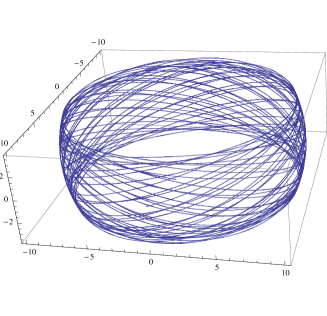
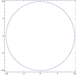
Figure 1: A spherical orbit for mass ratio $m_{2}/m_{1}=1/4$ and spin amplitudes of $3/4$. Both spins are initially displaced from the orbital angular momentum by $\pi/4$. Notice the orbit is not closed. Upper Panel: The three-dimensional orbit fills out a strip on a sphere. If we waited long enough, the band would be solidly painted, a reflection of the aperiodicity of the orbit. Lower Panel: The path as caught by the orbital plane reveals the constant radius.

In this companion to paper I, we work again in the conservative Hamiltonian 3PN approximation plus spin-orbit coupling, but move beyond paper I to consider two spinning black holes in a binary. We focus on special sets of orbits, namely the spherical orbits. That might seem ironic since we have just argued that gravitational wave science will probe the full range of dynamical possibilities, there are several good reasons to devote some time to constant radius orbits.

1. If even one black hole spins, the constant radius orbits are no longer circles (unless spins are exactly aligned or anti-aligned with the orbital angular momentum) damoureob2001 ; buonanno2006 . As a result of spin precession, they fill a band on the surface of a sphere and have thereby been coined spherical orbits (see Fig. 1). Long-lived binaries that have shed enough angular momentum to lose their eccentricity but not their spin will exhibit quasi-spherical inspiral and not quasi-circular inspiral. To detect waves from realistic binaries, we will need to understand the orbital parameters and precessions of these spherical orbits.

2. Black hole pairs that enter the LIGO bandwidth with their eccentricity intact will evolve through a sequence of zoom-whirl orbits rather than nearly spherical ones. Still, the spherical sets are special since they mark the minimum and maximum energy in the strong-field spectrum of bound orbis for a given angular momentum. The orbital demographic is therefore entirely determined by the spherical orbits levin2008:2 .

3. The energetically-bound unstable spherical orbits mark the divide between inspiral and plunge Sperhake:2007gu . More specifically, black hole spacetimes harbor homoclinic orbits – orbits that approach the unstable spherical orbits in the infinite future or in the infinite past bombelli1992 ; levino2000 ; levin2008:3 ; perez-giz2008 . A Homoclinic orbit, often refered to as a separatrix, is a classic feature of a non-linear dynamical system and deserve attention since they mark the transition from inspiral to plunge for all pairs. As we mention in the close of this paper, when spin-spin coupling is incorporated in the PN Hamiltonian, the homoclinic set can become the locus of a transition from regular to chaotic behavior.

Among the infinite list of spherical orbits, two are valuable enough to deserve names: the innermost stable spherical orbit (isso) and the innermost bound spherical orbit (ibso). The acronyms are drawn in analogy with the equatorial isco (innermost stable circular orbit) and ibco (innermost bound circular orbits). The isso is the lowest energy spherical orbital and the ibso is the highest energy, bound spherical orbit.

The isco, well-known as the site of the transition from inspiral to plunge for quasi-circular inspiral, is actually the zero eccentricity homoclinic orbit bombelli1992 . All other orbits, besides the quasi-circular one, will transition to plunge through another member of the homoclinic family, hence the importance of the homoclinic set to gravitational wave science levin2008:3 ; perez-giz2008 . To our knowledge the homoclinic orbits have not yet been identified in the PN Hamiltonian expansion before this paper, although an earlier paper found homoclinic orbits and zoom-whirl behavior in a hybrid PN expansion levino2000 . Excitingly enough, homoclinic orbits have been observed in fully relativistic, numerical treatments as well pretorius2007 .

Taken together this special set – composed of spherical and homoclinic orbits – demarcates dynamical regions and we spend time on their attributes in this paper. Due to the lack of confidence in the PN expansion at close separations, we do not advocate that these results be taken as quantitatively accurate descriptions of binary black hole dynamics, but rather as qualitatively descriptive. Ineed, we point out peculiar artifacts of the 3PN system as we go along and the results of this paper could provide a new terrain on which to test the PN expansion against, for instance, numerical relativity.

Our approach has some overlap with, but is not redundant with, the Refs. damoureob2001 ; buonanno2006 and allows us to find homoclinic orbits and stability exponents for use in the periodic orbit taxonomy of paper I levin2008:2 . We also simplify the initial conditions for spherical orbits in the absence of radiation reaction. For quasi-spherical orbits with radiation reaction included see buonanno2006 .

The outline of the paper is as follows: In §I we write out the equations of motion for two spinning bodies in an orbital basis, relying on the results of appendix A. In §II we determine the orbital parameters of spherical orbits. In §III we find the homoclinic orbits and emphasize their connection to dynamical instability. In the conclusion, §IV, we discuss the destruction of the spherical orbits and the transition to chaos when spin-spin coupling is included.

I 3PN Hamiltonian + SO Coupling

We will work with a condensed and revealing set of equations of motion in a non-orthogonal orbital coordinate system as derived in levin2008:2 . For reference in this companion to that paper, we write out the usual 3PN Hamilton plus spin-orbit coupling for two spinning black holes.

In a Hamiltonian formulation, the equations of motion are derived from

$$\dot{{\bf r}}=\frac{\partial H}{\partial{{\bf p}}}\quad,\quad\dot{{\bf p}}=-\frac{\partial{H}}{\partial{{\bf r}}}\quad.$$ (1)

As is standard convention, we work in dimensionless coordinates: the dimensionless coordinate vector, ${\bf r}$, is measured in units of total mass, $M=m_{1}+m_{2}$, for a pair with black hole masses $m_{1}$ and $m_{2}$. The canonical momentum, ${\bf p}$, is measured in units of the reduced mass, $\mu=m_{1}m_{2}/M$. The dimensionless combination $\eta=\mu/M$ will prove useful. We write vector quantities in bold. The coordinate $r$ is to be understood as the magnitude $r=\sqrt{{\bf r}\cdot{\bf r}}$. Unit vectors such as ${\bf{\hat{n}}}={\bf r}/r$ will additionally carry a hat. Finally, we have used the dimensionless reduced Hamiltonian $H={\cal H}/\mu$ in Eqs. (1), where ${\cal H}$ is the physical Hamiltonian, to 3PN order plus spin-orbit terms schaefer1985 ; damour1981 ; damour1988 ; jaranowski1998 ; damourpn2001 ; damourpn2000:2 . $H$ can be expanded as

$$H=H_{N}+H_{1PN}+H_{2PN}+H_{3PN}+H_{SO}\quad,$$ (2)

where

$$H_{N} =\frac{{{\bf p}}^{2}}{2}-\frac{1}{r}$$ (3)

$$H_{1PN} =\frac{1}{8}\left(3\eta-1\right)\left({{\bf p}}^{2}\right)^{2}-\frac{1}{2}\left[\left(3+\eta\right){{\bf p}}^{2}+\eta({{\bf{\hat{n}}}}\cdot{\bf p})^{2}\right]\frac{1}{r}+\frac{1}{2r^{2}}$$

$$H_{2PN} =\frac{1}{16}\left(1-5\eta+5\eta^{2}\right)\left({{\bf p}}^{2}\right)^{3}+\frac{1}{8}\left[\left(5-20\eta-3\eta^{2}\right)\left({{\bf p}}^{2}\right)^{2}\right.$$

$$\left.-2\eta^{2}({{\bf{\hat{n}}}}\cdot{{\bf p}})^{2}{{\bf p}}^{2}-3\eta^{2}({{\bf{\hat{n}}}}\cdot{{\bf p}})^{4}\right]\frac{1}{r}$$

$$+\frac{1}{2}\left[\left(5+8\eta\right){{\bf p}}^{2}+3\eta({{\bf{\hat{n}}}}\cdot{{\bf p}})^{2}\right]\frac{1}{r^{2}}-\frac{1}{4}\left(1+3\eta\right)\frac{1}{r^{3}}$$

$$H_{3PN} =\frac{1}{128}\left(-5+35\eta-70\eta^{2}+35\eta^{3}\right)\left({{\bf p}}^{2}\right)^{4}+\frac{1}{16}\left[\left(-7+42\eta-53\eta^{2}-5\eta^{3}\right)\left({{\bf p}}^{2}\right)^{3}\right.$$

$$\left.+(2-3\eta)\eta^{2}({{\bf{\hat{n}}}}\cdot{{\bf p}})^{2}({{\bf p}}^{2})^{2}+3(1-\eta)\eta^{2}({{\bf{\hat{n}}}}\cdot{{\bf p}})^{4}{{\bf p}}^{2}-5\eta^{3}({{\bf{\hat{n}}}}\cdot{{\bf p}})^{6}\right]\frac{1}{r}$$

$$+\left[\frac{1}{16}(-27+136\eta+109\eta^{2})({{\bf p}}^{2})^{2}+\frac{1}{16}(17+30\eta)\eta({{\bf{\hat{n}}}}\cdot{{\bf p}})^{2}{{\bf p}}^{2}+\frac{1}{12}(5+43\eta)\eta({{\bf{\hat{n}}}}\cdot{{\bf p}})^{4}\right]\frac{1}{r^{2}}$$

$$+\left\{\frac{1}{192}\left[-600+\left(3\pi^{2}-1340\right)\eta-552\eta^{2}\right]{{\bf p}}^{2}-\frac{1}{64}\left(340+3\pi^{2}+112\eta\right)\eta({{\bf{\hat{n}}}}\cdot{{\bf p}})^{2}\right\}\frac{1}{r^{3}}$$

$$+\frac{1}{96}\left[12+\left(872-63\pi^{2}\right)\eta\right]\frac{1}{r^{4}}\quad,$$

$$H_{SO} =\frac{{\bf L}\cdot{\bf S_{eff}}}{r^{3}}\quad.$$ (4)

For two spinning black holes ${\bf S_{eff}}$ is

$${\bf S_{eff}}=\delta_{1}{\bf S_{1}}+\delta_{2}{\bf S_{2}}$$ (5)

where the dimensionless reduced spins are defined as

$${\bf S_{1}}={\bf a_{1}}(m_{1}^{2}/\mu M)\quad,\quad\quad{\bf S_{2}}={\bf a_{2}}(m_{2}^{2}/\mu M)\quad.$$ (6)

and

$$\delta_{1}\equiv\left(2+\frac{3m_{2}}{2m_{1}}\right)\eta\quad,\quad\quad\delta_{2}\equiv\left(2+\frac{3m_{1}}{2m_{2}}\right)\eta\quad.$$ (7)

The dimensionless spin amplitudes are confined to the range $0\leq a_{1,2}\leq 1$. The reduced orbital angular momentum ${\bf L}={\bf r}\times{\bf p}$ and the spins precess according to

$${\bf\dot{\bf L}} = \frac{{\bf S_{eff}}\times\bf L}{r^{3}}$$

$${\bf\dot{{\bf S}}_{1}} = \delta_{1}\frac{{\bf L}\times{\bf S_{1}}}{r^{3}}$$

$${\bf\dot{{\bf S}}_{2}} = \delta_{2}\frac{{\bf L}\times{\bf S_{2}}}{r^{3}}\quad.$$ (8)

The spin precessions can be grouped together,

$${\bf\dot{{\bf S}}_{1}}+{\bf\dot{{\bf S}}_{2}} = \frac{{\bf L}\times{\bf S_{eff}}}{r^{3}}\quad.$$ (9)

Notice that the precession of the sum of the spins is equal and opposite to the precession of the orbital angular momentum. So that ${\bf J}={\bf L}+{\bf S_{1}}+{\bf S_{2}}$ is conserved. The magnitudes $L,S_{1}$ and $S_{2}$, the inner product ${\bf S_{eff}}\cdot{\bf L}$, and the energy (the Hamiltonian) are also constant for a given orbit.

In general, neither ${\bf{\hat{J}}}\cdot{\bf{\hat{L}}}$ nor the magnitude $|S_{\rm eff}|$ is constant. However, there are notable exceptions gopakumar2005 . Both ${\bf{\hat{J}}}\cdot{\bf{\hat{L}}}$ and the magnitude $|S_{\rm eff}|$ are constant (1) if one of the black holes is spinless as was the case in levin2008:2 , (2) if the binaries have exactly equal mass gopakumar2005 , or (3) if both spins are aligned or anti-aligned with the angular momentum. Case (1) is worked out thoroughly in paper I levin2008:2 . To see that the claim is true in the equal mass case (2), notice that ${\bf S_{eff}}=\delta_{1}({\bf S_{1}}+{\bf S_{2}})$ and therefore ${\bf J}={\bf L}+{\bf S_{eff}}/\delta_{1}$. Consequently, ${\bf J}\cdot{\bf L}=L^{2}+{\bf S_{eff}}\cdot{\bf L}/\delta_{1}$ is conserved since both terms on the right hand side are conserved. Furthermore, ${\bf\dot{{\bf S}}_{\rm eff}}=\delta_{1}({\bf\dot{{\bf S}}_{1}}+{\bf\dot{{\bf S}}_{2}})$ and it follows from Eq. (9) that the change in ${\bf S_{eff}}$ is always perpendicular to ${\bf S_{eff}}$ so its magnitude remains constant. In case (3), when the spins are aligned or anti-aligned with the orbital angular momentum, motion is confined to a plane and there is no precession. Therefore ${\bf S_{eff}}$ and ${\bf L}$ are constants and the rest follows.

The results of this paper will apply to a general ${\bf S_{eff}}$ unless explicitly stated otherwise.

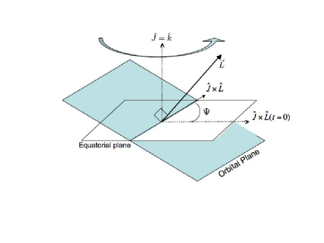
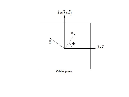
Figure 2: Upper: The orbital plane precesses around the ${\bf{\hat{J}}}={\bf{\hat{k}}}$ axis through the angle $\Psi$. Lower: The orbital plane can be spanned by the vectors $({\bf{\hat{n}}},{\bf{\hat{\Phi}}})$.

I.1 Equations of Motion in the Orbital Plane

In a non-orthogonal orbital basis, the equations of motion assume a simple form that allows us to analyze the dynamics of the black hole pairs. The plane perpendicular to the precessing orbital angular momentum is spanned by the vectors $({\bf{\hat{n}}},{\bf{\hat{\Phi}}})$ where ${\bf{\hat{n}}}={\bf r}/r$ and

$${\bf{\hat{\Phi}}}={\bf{\hat{L}}}\times{\bf{\hat{n}}}\quad.$$ (10)

Notice ${\bf{\hat{n}}}\cdot{\bf{\hat{\Phi}}}=0$ so these basis vectors are orthogonal. The entire orbital plane then precesses around the constant total angular momentum ${\bf J}={\bf L}+{\bf S_{1}}+{\bf S_{2}}$ in the direction ${\bf{\hat{\Psi}}}$ defined through

$${\bf{\hat{\Psi}}}={\bf{\hat{J}}}\times\frac{({\bf{\hat{J}}}\times{\bf{\hat{L}}})}{\left|{\bf{\hat{J}}}\times{\bf{\hat{L}}}\right|}\quad.$$ (11)

The construction, familiar from classical celestial mechanics schafer1993 ; wex1998 ; gong2004 ; konigsdorffer2005 , is illustrated in Fig. 2. Incidentally, this basis is explicitly constructed for ${\bf J}\times{\bf L}\neq 0$. When the spin and orbital angular momentum are aligned, anti-aligned, or spin is zero then ${\bf J}\times{\bf L}=0$, motion is confined to a plane, and we should use the usual equatorial planar basis.

Notice that ${\bf{\hat{\Psi}}}$ is not orthogonal to the orbital plane and therefore our orbital basis $({\bf{\hat{n}}},{\bf{\hat{\Phi}}},{\bf{\hat{\Psi}}})$ is not orthogonal.

From Eq. (1), we can find equations of motion in coordinates $(r,\Phi,\Psi)$ and their canonical momenta $(P_{r},P_{\Phi},P_{\Psi})$. As in appendix A, where we follow the approach of paper I, it is convenient to first isolate the equations of motion in the orbital plane for the variables $(r,\Phi)$ and their canonical momenta $(P_{r},P_{\Phi})$:

$$\dot{r} =AP_{r}+B\,,\qquad \dot{P}_{r} =A\frac{P_{\Phi}^{2}}{r^{3}}+CP_{r}+D+3P_{\Phi}\frac{{\bf S_{eff}}\cdot{\bf{\hat{L}}}}{r^{4}}$$ (12)

$$\dot{\Phi} =A\frac{P_{\Phi}}{r^{2}}+\frac{{\bf S_{eff}}\cdot{\bf{\hat{L}}}}{r^{3}}-\dot{\Psi}({\bf{\hat{J}}}\cdot{\bf{\hat{L}}})\,,\qquad \dot{P}_{\Phi} =0$$

where $A,B,C,D$ are functions of $(r,P_{r})$ to be defined momentarily. The momentum $P_{\Phi}=L$ conjugate to $\Phi$ is conserved, by the justification in paper I which survives despite the addition of a second spin. In any other basis, although $L$ is constant, it is not a momentum conjugate to any coordinate. Instead, $L$ should be interpreted in terms of the linearly independent coordinates and momenta appropriate for that basis. The added beauty of this non-orthogonal approach is that $L$ is a canonical momentum, namely $P_{\Phi}$, not so in the usual spherical coordinate basis where $L$ is neither a coordinate nor a momentum and the Hamiltonian angular equations of motion are less transparent.

The four Eqs. (12) describe motion within the orbital plane. The orbital plane itself precesses around the constant ${\bf{\hat{J}}}$ with variable rate $\dot{\Psi}$, derived in appendix A.2 to be

$$\dot{\Psi}=\left(\frac{{\bf{\hat{J}}}\times\left({\bf S_{eff}}\times{\bf{\hat{L}}}\right)}{\left|{\bf{\hat{J}}}\times{\bf{\hat{L}}}\right|r^{3}}\right)\cdot{\bf{\hat{\Psi}}}\,,\quad\dot{P}_{\Psi}=\left(\frac{{\bf S_{eff}}\times{\bf{\hat{L}}}}{r3}\right)\cdot{\bf{\hat{J}}}\quad,$$ (13)

and $P_{\Psi}={\bf L}\cdot{\bf{\hat{J}}}=L_{z}$ is not a constant.

Again, using the manipulations of appendix A, particularly Eq. (52) and the identities ${\bf{\hat{J}}}\cdot{\bf{\hat{L}}}=\cos\theta_{L}=P_{\Psi}/P_{\Phi}$, $|{\bf{\hat{J}}}\times{\bf{\hat{L}}}|=\sin\theta_{L}$, we can write the final term in the $\dot{\Phi}$ equation of (12) as

$$\dot{\Psi}({\bf{\hat{J}}}\cdot{\bf{\hat{L}}})=\left(\frac{\left({\bf S_{eff}}\cdot{\bf{\hat{J}}}\right)-\left({\bf S_{eff}}\cdot{\bf{\hat{L}}}\right)P_{\Psi}/P_{\Phi}}{\left(1-(P_{\Psi}/P_{\Phi})^{2}\right)r^{3}}\right)\frac{P_{\Psi}}{P_{\Phi}}\quad.$$ (14)

Writing it in this form exploits the dependences on the coordinates, conjugate momenta, and the constant ${\bf S_{eff}}\cdot{\bf{\hat{L}}}$. The one term that clearly remains dependent on angles is the term ${\bf S_{eff}}\cdot{\bf J}$. Therefore, when both black holes spin, the angular equations will depend on the angular precession of the orbital plane.

We saw in paper I a dramatic simplification in the case of one effective spin. As follows from the earlier discussion of the constants of motion, ${\bf S_{eff}}\cdot{\bf{\hat{J}}}$ would be constant if either of the spins vanished and this would remove the angular depedence in the above equations. A pair of spinning black holes of equal mass is also reducible to a system with effectively one spin (see §A.3). We continue to consider the general case of two misaligned spins for arbitrary mass ratios.

For completeness, and as a complement to paper I, we explicitly write out the functions $A,B,C,D$ that were set up in levin2008:2 as derivatives on the Hamiltonian:

$$A=1+ \frac{1}{2}\left(3\eta-1\right){\bf p}^{2}-\left(3+\eta\right)\frac{1}{r}+$$

$$\frac{3}{8}\left(1-5\eta+5{\eta}^{2}\right)\left({\bf p}^{2}\right)^{2}+\frac{1}{4}\left[2\left(5-20\eta-3{\eta}^{2}\right){\bf p}^{2}-2{\eta}^{2}\left({\bf{\hat{n}}}\cdot{\bf p}\right)^{2}\right]\frac{1}{r}+\left(5+8\eta\right)\frac{1}{r^{2}}$$

$$\frac{1}{16}\left(-5+35\eta-70{\eta}^{2}+35{\eta}^{3}\right)\left({\bf p}^{2}\right)^{3}+$$

$$\frac{1}{8}\left[3\left(-7+42\eta-53\eta^{2}-5\eta^{3}\right)({\bf p}^{2})^{2}+2\left(2-3\eta\right){\eta}^{2}\left({\bf{\hat{n}}}\cdot{\bf p}\right)^{2}{\bf p}^{2}+3\left(1-\eta\right){\eta}^{2}\left({\bf{\hat{n}}}\cdot{\bf p}\right)^{4}\right]\frac{1}{r}+$$

$$\left[\frac{1}{4}\left(-27+136\eta+109{\eta}^{2}\right){\bf p}^{2}+\frac{1}{8}\left(17+30\eta\right)\eta\left({\bf{\hat{n}}}\cdot{\bf p}\right)^{2}\right]\frac{1}{r^{2}}+$$

$$2\left[-\frac{25}{8}+\left(\frac{1}{64}{\pi}^{2}-\frac{335}{48}\right)\eta-\frac{23}{8}\eta^{2}\right]\frac{1}{r^{3}}$$ (15)

$$B= -\eta\left({\bf{\hat{n}}}\cdot{\bf p}\right)\frac{1}{r}+$$

$$\frac{1}{8}\left[-4{\eta}^{2}\left({\bf{\hat{n}}}\cdot{\bf p}\right){\bf p}^{2}-12{\eta}^{2}\left({\bf{\hat{n}}}\cdot{\bf p}\right)^{3}\right]\frac{1}{r}+$$

$$3\eta\left({\bf{\hat{n}}}\cdot{\bf p}\right)\frac{1}{r^{2}}+$$

$$\frac{1}{16}\left[2\left(2-3\eta\right){\eta}^{2}\left({\bf{\hat{n}}}\cdot{\bf p}\right)\left({\bf p}^{2}\right)^{2}+12\left(1-\eta\right){\eta}^{2}\left({\bf{\hat{n}}}\cdot{\bf p}\right)^{3}{\bf p}^{2}-30{\eta}^{3}\left({\bf{\hat{n}}}\cdot{\bf p}\right)^{5}\right]\frac{1}{r}+$$

$$\left[\frac{1}{8}\left(17+30\eta\right)\eta\left({\bf{\hat{n}}}\cdot{\bf p}\right){\bf p}^{2}+\frac{1}{3}\left(5+43\eta\right)\eta\left({\bf{\hat{n}}}\cdot{\bf p}\right)^{3}\right]\frac{1}{r^{2}}+$$

$$2\left(-\frac{85}{16}-\frac{3}{64}{\pi}^{2}-\frac{7}{4}\eta\right)\eta\left({\bf{\hat{n}}}\cdot{\bf p}\right)\frac{1}{r^{3}}$$ (16)

$$C= -\frac{B}{r}$$ (17)

$$D= -({\bf{\hat{n}}}\cdot{\bf p})C-\frac{1}{r^{2}}-\frac{1}{2}\left(\left(3+\eta\right){\bf p}^{2}+\eta\left({\bf{\hat{n}}}\cdot{\bf p}\right)^{2}\right)\frac{1}{r^{2}}+\frac{1}{r^{3}}+$$

$$\frac{1}{8}\left[\left(5-20\eta-3{\eta}^{2}\right)\left({\bf p}^{2}\right)^{2}-2{\eta}^{2}\left({\bf{\hat{n}}}\cdot{\bf p}\right)^{2}{\bf p}^{2}-3{\eta}^{2}\left({\bf{\hat{n}}}\cdot{\bf p}\right)^{4}\right]\frac{1}{r^{2}}+$$

$$\left[\left(5+8\eta\right)\left({{\bf p}}^{2}\right)+3\eta\left({\bf{\hat{n}}}\cdot{\bf p}\right)^{2}\right]\frac{1}{r^{3}}-\frac{3}{4}\left(1+3\eta\right)\frac{1}{r^{4}}+$$

$$\frac{1}{16}\left[\left(-7+42\eta-53\eta^{2}-5\eta^{3}\right)({\bf p})^{3}+\left(2-3\eta\right){\eta}^{2}\left({\bf{\hat{n}}}\cdot{\bf p}\right)^{2}\left({\bf p}^{2}\right)^{2}+3\left(1-\eta\right){\eta}^{2}\left({\bf{\hat{n}}}\cdot{\bf p}\right)^{4}{\bf p}^{2}-\right.\left.5{\eta}^{3}\left({\bf{\hat{n}}}\cdot{\bf p}\right)^{6}\right]\frac{1}{r^{2}}+$$

$$2\left[\frac{1}{16}\left(-27+136\eta+109{\eta}^{2}\right)\left({\bf p}^{2}\right)^{2}+\frac{1}{16}\left(17+30\eta\right)\eta\left({\bf{\hat{n}}}\cdot{\bf p}\right)^{2}{\bf p}^{2}\right.+$$

$$\left.\frac{1}{12}\left(5+43\eta\right)\eta\left({\bf{\hat{n}}}\cdot{\bf p}\right)^{4}\right]\frac{1}{r^{3}}+3\left\{\left[-\frac{25}{8}+\left(\frac{1}{64}{\pi}^{2}-\frac{335}{48}\right)\eta-\frac{23}{8}\eta^{2}\right]{\bf p}^{2}+\right.$$

$$\left.\left(-\frac{85}{16}-\frac{3}{64}{\pi}^{2}-\frac{7}{4}\eta\right)\eta\left({\bf{\hat{n}}}\cdot{\bf p}\right)^{2}\right\}\frac{1}{r^{4}}+4\left[\frac{1}{8}+\left(\frac{109}{12}-\frac{21}{32}{\pi}^{2}\right)\eta\right]\frac{1}{r^{5}}$$ (18)

where ${\bf{\hat{n}}}\cdot{\bf p}=P_{r}$ and ${\bf p}^{2}=P_{r}^{2}+L^{2}/r^{2}$. Notice that $A,B,C,D$, which come from the non-spinning part of the Hamiltonian levin2008:2 , depend only on $(r,P_{r})$ and constants.

Useful results can be drawn from a simple observation. The radial equations in (12) have no angular dependence. The energy, angular momentum, and radius of spherical orbits can be derived from the radial equations alone. Therefore we can find spherical orbits simply despite the precession of the orbital plane.

The fact that the two equations in $(r,P_{r})$ form a self-contained system is a restatement of the fact that the Hamiltonian itself can be viewed in a one-dimensional effective approach as a function of $(r,P_{r})$ and constants. It is important to be cautious however when investigating the angular motion. The Hamiltonian depends only on $(r,P_{r})$ and constants in time, yet those constants in time have to be carefully varied as functions of the angular coordinates and their conjugate momenta in a given basis to correctly derive the remaining equations of motion. This accounts for the labor in appendix A needed to derive the $(\Phi,P_{\Phi})$ and $(\Psi,P_{\Psi})$ equations of motion.

Still, the simple dependences of the Hamiltonian allows us to analyze the spherical orbits as one-dimensional radial motion in a simple effective potential. The location of the spherical orbits was implicit in paper I to frame the distribution of all other orbits. For completeness we determine the range of spherical orbits with an eye on that companion work.

II Spherical Orbits

II.1 Effective Potential for Spinning Black Holes

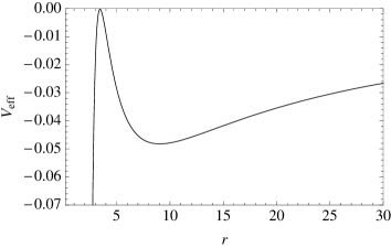
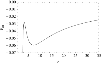
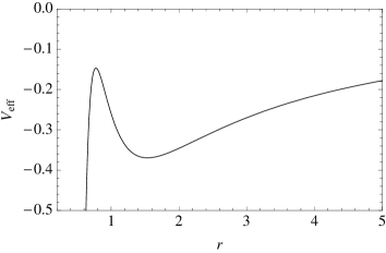
Figure 3: An effective potential for two spinning black holes $a_{1}=a_{2}=3/4$ of mass ratio $m_{2}/m_{1}=1/4$ for different values of the angular momentum. Notice the change in scale between panels. Upper: The appearance of the ibso is marked by the effective potential touching the line $H=0$. Next: As the angular momentum decreases, the potential will have both stable and unstable spherical orbits. Next: As the angular momentum is further decreased there occurs a critical value at which the unstable and stable spherical orbits merge at a saddle point, the isso. Lower: The last panel shows a difference from the Schwarzschild or Kerr stories. At angular momenta and radii below the occurence of the isso, there occur new sets of stable and unstable spherical orbits. These occur at radii far below which the approximation can be trusted, yet we point out their presence for completeness.

Ideally, in an effective potential formulation, the radial equation could be cast in the form:

$$\frac{1}{2}\dot{r}^{2}+{\rm effective\ potential}={\rm constant}$$ (19)

where the effective potential depends only on $r$ and constants of the motion. Now, the Hamiltonian of Eqs. (2)-(4) does not admit a simple effective potential formulation since it is a complicated function of ${\bf p}^{2}$. We have already argued that $H(r,{\bf p},{\bf S_{eff}})$ can be written as an effective function of $(r,P_{r})$ and constants, yet it remains a polynomial function of $P_{r}$. However, if we only consider

$$V_{\rm eff}=H({P_{r}=0})\quad,$$ (20)

then we have a good representation of a pseudo effective-potential at the turning points. We cannot misuse the $V_{\rm eff}$ by trying to interpret motion away from the turning points, but it gives a perfectly valid description of the behavior at aphelia and periastra as well as on spherical orbits. Hereafter we’ll shorthand the term “pseudo effective-potential” by “effective potential”.

From the Hamiltonian of Eqs. (4), the effective potential,

$$V_{\rm eff}(r,L,{\bf S_{eff}}\cdot{\bf{\hat{L}}},\eta)\quad\quad,$$ (21)

is a function of orbital parameters $(r,L,{\bf S_{eff}}\cdot{\bf{\hat{L}}})$ and the mass ratio. Again, since $L$ and ${\bf S_{eff}}\cdot{\bf{\hat{L}}}$ are constants of the motion, for a given $(L,{\bf S_{eff}}\cdot{\bf{\hat{L}}})$ and a given mass ratio, the potential is a function of $r$ only.

Fig. 3 shows several snapshots taken of the effective potential for a pair of spinning black holes as the magnitude of $L$ decreases for a given ${\bf S_{eff}}\cdot{\bf{\hat{L}}}$ value. (For a detailed exposition on interpreting effective potentials for black hole orbits see Refs. wald1984 and levin2008:3 ; perez-giz2008 .) The spherical orbits are simply the extrema of the potential. An example of such an orbit was shown in Fig. 1. Although this orbit is not generally periodic, it does close in the orbital plane as shown in the lower panel of Fig. 1.

The top panel of Fig. 3 marks the value of $L$ for which a margnially bound, unstable spherical orbit appears. An orbit is marginaly bound if its energy $H=0$ and it is spherical and unstable if it is a maximum of the effective potential. The conditions are summarized as

$$V_{\rm eff}(P_{r}=0) =0$$

$$\frac{\partial V_{\rm eff}}{\partial r} =0$$

$$\frac{\partial^{2}V_{\rm eff}}{\partial r^{2}} <0\quad\quad\quad({\rm ibso}),$$ (22)

although the first two are sufficient. We call the margnially bound unstable spherical orbit “ibso” in analogy with the innermost unstable circular orbit (ibco) of equatorial orbits.

For angular momenta below $L_{\text{ibso}}$ there will be both a stable and unstable, energetically bound spherical orbit, as in the second snapshot of Fig. 3, until the angular momentum gets so low that we reach the third snapshot from the top. Here, the unstable and stable spherical orbits have merged in a saddle point, coined an innermost stable spherical orbit (isso):

$$\frac{\partial V_{\rm eff}}{\partial r} =0$$

$$\frac{\partial^{2}V_{\rm eff}}{\partial r^{2}} =0\quad\quad\quad({\rm isso}).$$ (23)

The story plotted out by panels 1-3 of Fig. 3 for $L_{\text{isso}}<L<L_{\text{ibso}}$ qualitatively follows the fully relativistic Schwarzaschild and Kerr stories as expected levin2008:3 ; perez-giz2008 . However, something peculiar then happens in the PN approximation at very low values of the angular momentum. New stable and unstable spherical orbits can appear as shown in the bottom panel of Fig. 3. Or, for some other ranges of parameters, the ibso disappears or the isso disappears or both disappear. Sometimes these problems occur, as in the figure, for radii far below the confidence of the PN approximation. We point out these troublesome features in the spirit of full disclosure. More than this, the details provide a quantitative testing ground for the approximation.

Despite these oddities at low $r$ where the PN-approximation would make no claims of quantitative validity anyway, the qualitative features of spherical orbits, homoclinic orbits, and zoom-whirl behavior should survive improved approximations and full numerical treatments Pretorius2006 . We will locate the $E$ and $L$ of spherical orbits in the next subsection.

II.2 Orbital Parameters for Spherical Orbits

For a given black hole pair, that is, a given mass ratio and ${\bf S_{eff}}\cdot{\bf{\hat{L}}}$, all orbits are uniquely specified by their $(E,L)$. Using the effective potential, we can easily generate the $E$ and $L$ for spherical orbits and thereby generate initial data for them. Initial conditions for spherical orbits were also found in damoureob2001 ; buonanno2006 . Damour damoureob2001 noticed that when only spin-orbit terms are included that the Hamiltonian could be expressed as a radial function. One could arrive at this conclusion, as we have in the previous section. The constant radius orbits occur at the extrema of $H(r,P_{r})$, in the same spirit as an effective potential method.

Figure 4: $(m_{2}/m_{1}=10^{-6},S_{\rm eff}=0)$. Upper: Angular momentum vs $r_{s}$. Lower: Energy vs $r_{s}$.

From the vantage point of the effective potential, spherical orbits satisfy the condition

$$\frac{\partial V_{\rm eff}}{\partial r}=0$$ (24)

treating $L$ and ${\bf S_{eff}}\cdot{\bf{\hat{L}}}$ as constants. We could also take the vantage point of the equations of motion. Since, $P_{r}=0$ forces $B=0$, the condition $\dot{r}=AP_{r}+B=0$ can be thought of as synonymous with the condition that $P_{r}=0$. The constant radius condition is thus the requirement that

$$\left.\dot{P}_{r}\right|_{P_{r}=0}=0$$ (25)

in Eqs. (12) and Eq. (25) is equivalent to Eq. (24).

The roots of the 8th-order equation in $L$, Eq. (25), give the angular momenta of the spherical orbits as a function of spherical radius, $L_{s}(r_{s})$, where we use a subscript $s$ to denote a quantity evaluated at a spherical orbit. (When there is no spin, the condition reduces to a quartic in $L^{2}$ with only two of the four roots real.) Piecing together the real roots we find $L_{s}$’s such as the one in Fig. 4. Although the upper branch grows very quickly in $L_{s}$, these values rapidly become physically unreachable since it would require angular velocities greater than the speed of light to be that high up on the upper branch. One can think of $(L_{s}/r_{s})<1$ as a crude marker of physically allowed values. To find the energy of spherical orbits, $E_{s}(r_{s})$, we simply plug $L_{s}(r_{s})$ into the Hamiltonian when $P_{r}=0$. The energy plot is also shown in Fig. 4.

There are several things to notice about the $L_{s}$ and $E_{s}$ plots, for which we chose values to illustrate the PN approximation to Schwarzschild $(m_{2}/m_{1}=10^{-6},S_{\rm eff}=0)$. The large values of $r_{s}$ correspond to stable spherical orbits. (Since spin is zero, these constant radius orbits are actually circular equatorial but we’ll keep the language more general.) When $L_{s}$ hits a minimum, we have found the isso – for no $L<L_{\text{isso}}$ are there spherical orbits. To the left of that minimum are the unstable spherical orbits. A true peculiarity of the figure is the fact that the radii of the unstable spherical orbits begin to move out to larger $r$. This is simply a flaw in the PN approximation and does not occur in the Schwarzschild system. In the fully relativistic system the unstable spherical orbits always move to smaller radii than the isco, hence the ibco is really innermost, earning its name. Here, the ibso is not actually innermost – due to the poor quality of the approximation – although it remains the highest energy bound spherical orbit when it exists. The ibso cannot be read off of Fig. 4 although it can be found simply as the coincident of the roots of Eqs. (22).

Figs. 4 are for a non-spinning extreme-mass-ratio binary and are therefore valid as an approximation to Schwarzschild. The details of these figures will be useful for a future test of the PN expansion. Here we note that $L_{\text{ibso}}\approx 4.69$, which is about $17$% higher than the Schwarzschild value of $4$ while $L_{\text{isso}}\approx 3.75$, which is about $8$% higher than the Schwarzschild value of $\sqrt{12}$. The energy of the ibso is designed to be zero so is not informative but the energy of the isso is $E_{\text{isso}}\approx-0.0452$, which is about $21$% less negative, that is less energetically bound, than the Schwarzschild case $(2\sqrt{2}/3)-1$. Due to the approximate nature of the expansion it is not necessary to take these comparisons to heart, but they indicate how the spherical orbits and the periodic spectra could facillitate a test of the PN expansion. For a comparison of the isso in different PN approaches including the resummed Kerr-like effective-one-body approach see damourpn2000:2 ; buonanno2006 .

Figure 5: All black hole pairs represented have ${\bf S_{eff}}\cdot{\bf{\hat{L}}}=0.35355$. Upper: Angular momentum vs $r$ for the ibso and isso for different mass ratios. The upper point is always the ibso for a given symbol while the lower point with the same symbol is always the isso. The key lists the different $(m_{2}/m_{1})$. Lower: Energy vs $r$.

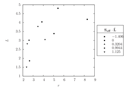
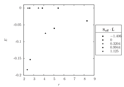
Figure 6: Upper: Angular momentum vs $r$ for the ibso and isso for fixed mass ratio $m_{1}/m_{1}=1/3$ but varying ${\bf S_{eff}}\cdot{\bf{\hat{L}}}$. The upper point is always the ibso for a given symbol while the lower point with the same symbol is always the isso. The key lists ${\bf S_{eff}}\cdot{\bf{\hat{L}}}$. Lower: Energy vs $r$.

II.3 Dependence of Binding Energies on mass ratios and spin

For completeness, we can see how the ibso and the isso vary as the mass ratio and spins of the black holes are varied; that is, as their mass ratio and spins are varied. For one, since the ibso and isso frame the distribution of orbits, they define the ranges of $E$ and $L$ values for all other orbits in the strong-field. For another, the energy at the isso gives an estimate of the energy emitted on quasi-circular inspiral up to the transition to plunge. A larger binding energy at the isso could also mean a larger signal at final coalescence so these variations attest to various levels of detectability. We will discuss the binding energy of the isso in this section. In the next section we will consider the transition to plunge for eccentric orbits.

A black hole pair is specified by its mass ratio, $m_{2}/m_{1}$, and its spins through the particular combination ${\bf S_{eff}}\cdot{\bf{\hat{L}}}$. The Hamiltonian, and the radial equations, depend only on these two combinations. We will therefore consider the variations in the isso and ibso for black hole pairs distinguished only by their $(m_{2}/m_{1},{\bf S_{eff}}\cdot{\bf{\hat{L}}})$ values. It is important to realize that there is a great deal of degeneracy among pairs. The ibso and isso values (their energy, angular momenta, and radial values) are identical for two physically distinct black hole pairs. For instance, a black hole with mass ratio $m_{2}/m_{1}=1/3$ and ${\bf S_{eff}}\cdot{\bf{\hat{L}}}=0.35355$ could be a black hole with initial values $a_{1}=1/4$, $a_{2}=0$, and the spin of the heavier black hole aligned with the initial orbital angular momentum. However, this is not the only combination of spin amplitudes and angles that will give the combination ${\bf S_{eff}}\cdot{\bf{\hat{L}}}=0.35355$. While different black hole pairs can give degenerate isso and ibso values, they will be physically distinguishable through their angular motion.

In Fig. 5 the $L$ of the ibso and isso is plotted in the upper panel and the $E$ of the isso and of the ibso are plotted in the lower panel. Qualitative conclusions can be drawn from these figures. We notice that as the mass ratio is increased towards 1, the radius of both the isso and ibso decrease, although the isso moves in faster. Therefore the isso is pushed to larger binding energies as the mass ratio is increased towards 1. Because the Hamiltonian is a high-order polynomial in $r$, there can be more than one marginally bound orbit and more than one saddle point for a given $(m_{2}/m_{1},{\bf S_{eff}}\cdot{\bf{\hat{L}}})$ pair, as demonstrated in the lowest panel of Fig. 3. The second occurence of a marginally bound orbit and/or saddle point appears in the vicinity of $r\sim 1$ where the approximation is uninterpretable. (There may even be third occurences.) It is unclear if there is any physical content to these other stable and unstable spherical orbits. Fig. 5 plots only the ibso/isso pair for $r$ values $>2$.

For the value of ${\bf S_{eff}}\cdot{\bf{\hat{L}}}\sim 0.35355$ used in the figure, either the ibso or the isso disappears (or both disappear) as $m_{2}$ approaches $m_{1}$. There may still be very small radii $(r\sim 1)$ ibso’s and/or isso’s, but the sensible ones disappear. This peculiarity is probably an artefact of the approximation, a point we return to momentarily.

Fig. 6 fixes the mass ratio at $m_{2}/m_{1}=1/3$ and varies ${\bf S_{eff}}\cdot{\bf{\hat{L}}}$. Increasing ${\bf S_{eff}}\cdot{\bf{\hat{L}}}$ has the same effect of pushing the isso to smaller separations and therefore to larger binding energies, although again the isso moves in faster – discounting any marginally bound spherical orbit or saddle points that occur in the vicinity of $r\sim 1$. (In fact, as Fig. 6 shows, at some point the isso actually occurs at a smaller radius than the ibso.) So, all other factors being equal, spins anti-aligned with the orbital angular momentum push the isso out to larger radii and smaller binding energies while aligned spins pull the isso into smaller radii and larger binding energies. For the mass ratio of this figure, the ibso or the isso actually vanishes (or both vanish) as ${\bf S_{eff}}\cdot{\bf{\hat{L}}}$ is increased much beyond the values shown.

These trends are consistent with those for spherical orbits discussed in Ref.  buonanno2006 . For the equal mass case with spins aligned or anti-aligned with the orbital angular momentum, the authors of that reference also remarked on the absense of an isso (called a last stable spherical orbit (lsso) in their lexicon). Indeed, they used this failing to argue that the PN expansion could not be used to study the transition from inspirl to plunge and advocated instead the seemingly more reliable effective-one-body (EOB) approach buonanno1999 ; damoureob2001 ; buonanno2007 . It would be interesting to extend to the EOB method the investigation of the zoom-whirl orbits of paper I levin2008:2 and the homoclinic limit of the zoom-whirls that we turn to in the next section. We leave that to a future work and continue to use the 3PN Hamiltonian as an example of our general method.

The disappearance of the ibso accompanies the disappearance of all unstable spherical orbits. Once this happens, there can be no isso since the isso is really the point of merger of the unstable and stable spherical orbits. As is already known, in the absence of spin there are no bound unstable circular orbits at 2PN kidder1993 ; wex1993 ; schafer1993 ; Damour:1997ub ; buonanno1999 . At 3PN there are no bound unstable circular orbits for mass ratios bigger than about $m_{2}/m_{1}\sim 1/2$. (See also damourpn2000:2 ; blanchet2002 .) The absence of a bound unstable circular orbit is clearly a shortcoming of the approximation since we know that the Schwarzschild spacetime possess an unstable circular orbit as a reflection of its high non-linearity. Furthermore, the unstable circular orbits are present in fully relativistic treatments as the equal mass numerical investigation of Ref. Pretorius2006 shows. Therefore, the ibso and isso should emerge for $m_{2}\rightarrow m_{1}$ at higher orders. Incidentally, their disappearance at 3PN-order implies the expansion is very likely approximating the dynamics as more stable than it really is and therefore less vulnerable to chaos than it really is for these comparable mass binaries.

We have already warned caution to take the trends as qualitative indicators and not to invest too much in the numbers due to pressures on the PN expansion at such large values of $(m_{1}+m_{2})/r$. Afterall, the PN expansion is an expansion in small $(m_{1}+m_{2})/r$ and will naturally begin to faulter for small $r$.

We have focused on the binding energy of the isso primarily to fit into the wider conversation that has focused on quasi-circular inspiral. However, the eccentric binaries formed by tidal capture in dense regions will not transition from inspiral to plunge through the isso. Rather they will transition through the eccentric separatrix between bound and plunging orbits. We investigate that separatrix briefly in the final section.

III Homoclinic Orbits – the separatrix between bound and plunging orbits

It is worthwhile to mention another important kind of orbit that occurs in our dynamical system, the homoclinic orbit bombelli1992 ; levino2000 . Homoclinic orbits are intriguing for several reasons, not least of which is that they mark the orbits through which the transition from inspiral to plunge should occur. In fact, the isso itself, the transition point for quasi-circular orbits, is a zero eccentricity homoclinic orbit bombelli1992 ; levin2008:3 ; perez-giz2008 . We make the connection between the energetically bound, unstable spherical orbits and the homoclinic orbit explicit in this final section.

Formally, homoclinic orbits are defined as trajectories that asymptote to the same hyperbolic invariant set in the infinite future as in the inifinite past. In these black hole settings, the role of the hyperbolic invariant set is played by the energetically bound, unstable spherical orbits. Although in the lexicon of black hole physics these orbits have been coined “unstable”, they are strictly speaking hyperoblic, which is to say they possess both a stable eigendirection and an unstable eigendirection under linear perturbations. And, the eigendirections lie along the homoclinic orbit in the local neighborhood of the unstable circle they approach. Although we won’t demonstrate that line up here, the point was emphasized in detail in Refs. levin2008:3 ; perez-giz2008 for Kerr equatorial dynamics.

The stability exponents can be found by linearizing in small perturbations around Eqs. (12). This was done for equatorial Kerr orbits in Ref. perez-giz2008 . Although we will not write out the explicit procedure here, we mention that the spherical orbits have radial eigenvalues that come in plus/minus pairs, as they must in a Hamiltonian system. The radial eigenvalues are real for the unstable spherical orbits and imaginary for the stable spherical orbits. The isso occurs at the merger of the eigenvalues at zero. A direct computation of the stability exponents around circular orbits confirms that the stable spherical orbits and the unstable spherical orbits are distributed around the isso as Fig. 4 shows.

Figure 7: An effective-potential for $m_{2}/m_{1}=1/4$, with the spin of the heavier black hole displaced from ${\bf{\hat{L}}}$ by $\pi/4$ and amplitude $a_{1}=1/2$ while the lighter black hole has no spin. The straight line is the energy of the unstable spherical orbit. It is also the energy at another, larger turning point $r_{a}\sim 10$, which identifies the apaastron of the homoclinc orbit.

Through the phase space analysis we have shown that the energetically bound, unstable circular orbits are actually hyperbolic – they have a positive stability exponent as well as a negative stability exponent. We could compute the eigenvectors and show they lie along the homoclinic orbit in the local neighborhood of the unstable circle as we did for Kerr in Ref. perez-giz2008 . However, for our purposes it is sufficient and illuminating to consider a physical space picture.

We can identify the separatrix – i.e. the homoclinic orbit – in an effective-potential picture. In particular, consider a binary with mass ratio $m_{2}/m_{1}=1/4$ and the heavier black hole spins with amplitude $a_{1}=1/2$ offset from ${\bf{\hat{L}}}$ by $\pi/4$ while the lighter black hole is nonspinning. Although, again, any equivalent combination of ${\bf S_{eff}}\cdot{\bf{\hat{L}}}$ is described by this same figure. The unstable spherical orbit, $r_{u}$, at the maximum of $V_{\rm eff}$ in Fig. 7 is drawn in physical space in Fig. 8. Although the orbit is a closed circle in the orbital plane, it fills out a band on a sphere in three dimensions. Because of numerical instability near this orbit, we only show a few windings.

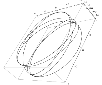
Figure 8: The unstable spherical orbit that is the maximum of $V_{\rm eff}$ for Fig. 7. Unlike the effective potential, the details of the full orbit do depend on the specific combination ${\bf S_{eff}}\cdot{\bf{\hat{L}}}$. Left: As viewed in three dimensions. Right: As viewed in the orbital plane.

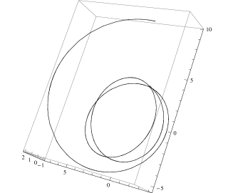
Figure 9: The homoclinic orbit for Fig. 7 approaching the unstable spherical orbit. Left: As viewed in 3d. Right: As viewed in the orbital plane. Because of numerical instability near the highly unstable constant radius orbit, we only show a few windings.

The energy of this orbit, $E_{s}(r_{u})$, is indicated by a straight line across the potential of Fig. 7. Note that this energy touches the potential at the unstable radius $r_{u}$ and at some larger radius, roughly $r\sim 10$. This larger radius is the apastron of an orbit. If the two black holes are released from rest at an initial separation in center-of-mass coordinates equal to this apastron, their orbit will roll down the potential (although the shape changes when $P_{r}\neq 0$) and then climb back up the other side asymptotically approaching the spherical orbit at the top of the hill. By definition, this is a homoclinic orbit (Fig. 9). To our knowledge it is the first of its kind to be found out of the equatorial plane levin2008 ; levin2008:3 ; perez-giz2008 .

The orbit winds around the center of mass an infinite number of times as it asymptotically approaches the unstable spherical orbit. Although not strictly periodic – the homoclinic orbit never returns to apastron – it will be significant for the periodic tables levin2008 ; levin2008:2 as a maximum energy orbit for a given $L$ in the strong-field regime levin2008:3 ; perez-giz2008 .

IV Conclusions

This paper, as the second in a series, provides the energetic frame in which the periodic tables of paper I were set levin2008:2 . Although in support of paper I’s goals, the analysis of spherical orbits could be relevant to additional tests of the PN expansion for spinning black hole pairs and could have a place in the disucssion of initial values for numerical relativity. Additionally, we find the non-equatorial homoclinic orbits that whirl an infinite number of times as they asymptote to the unstable spherical orbit. The homoclinic spearatrix is important as defining the transition to plunge for all orbits, including eccentric and precessing orbits. It would be interesting to extend this study to the EOB method buonanno1999 ; damoureob2001 ; buonanno2007 in a future work.

In closing, we comment on an intriguing implication of the set of spherical orbits for spinning black hole pairs. In this work, we restricted ourselves to spin-orbit coupling and although we allowed both black holes to spin, we found that the spherical orbits constrain the range of allowed bound orbits in the following sense. For a given angular momentum, spin initial conditions, and mass ratio, the stable spherical orbit is the lowest energy geodesic and the unstable spherical orbit is the highest energy orbit in the strong-field – barring the failures of the approximation at these close separations. As we showed in paper I levin2008:2 , between these two spherical orbits lies an infinite set of orbits that are closed in the orbital plane. The periodic set corresponds to a subset of the rationals, with the rational identifying a given orbit increasing monotonically between the stable spherical orbit and the unstable spherical orbit. The homoclinic orbit is the infinite whirl limit of the periodic set and would be the final entry in a periodic table of orbits corresponding to the infinite limit of the rationals.

This pattern of a periodic set framed by constant radius orbits and limiting to the homoclinic is consistent with a picture that has emerged for Kerr black hole orbits levin2008 ; levin2008:3 ; perez-giz2008 . The consistency of the picture for two spining comparable mass black holes with the Kerr case is precisely what is surprising, or at least intriguing. The geodesics in a Kerr spacetime are known to be integrable carter1968 . There are enough constants of the motion to restrict trajectories to regular tori and prohibit chaotic mixing. As Poincaré intuited, the structure of the periodic orbits encodes the entire dynamics and the regularity of the system is in fact reflected in the regularity of the periodic spectrum. The simplicity of the spherical orbits and the periodic set they frame suggests that even when both black holes spin and are of comparable mass, there is no chaos – at least not in physically plausible regimes –if only spin-orbit coupling is included.

Put another way, homoclinic orbits are also a sign of non-linearity. They mark the intersection of the stable and unstable manifolds of a hyperbolic invariant set. They are the precursor to chaos in the sense that under perturbation, the homoclinic orbit breaks up into a homoclinic tangle and will be the locus of a fractal set of orbits ott ; perez-giz2008 . The fractal set is sometimes refered to as a strange repellor and is the analog for conservative systems of strange attractors in dissipative systems cornish1994 ; dettman1994 ; Cornish:1996yg ; levin2000 .

Systems with a regular set of periodic orbits that culminate in a homoclinic limit are not chaotic. However, the spinning pairs are vulnerable to chaos as evidenced by their very possesion of a homoclinic orbit. Indeed chaos has by now been well confirmed in the form of a fractal set when spin-spin coupling is included levin2000 ; levin2003 ; gopakumar2005 ; levin2006 ; wu2007 ; wu2008 . As suspected in Ref. hartl2005 , our work suggests that the emergence of chaos must be directly tracable to the spin-spin coupling. We conjecture that the transition to chaos could be witnessed through the destruction of the corresondence of the periodic set with the rationals when spin-spin coupling is turned on. The additional precessional effects of spin-spin coupling, we suggest, must destroy the homoclinic orbit, replace it with a homoclinic tangle – a fractal set of orbits – and induce chaotic scattering among geodesics in the vicinity.

Appendix A Projection the equations of motion onto the non-orthogonal orbital basis

A.1 The Orbital Plane Equations

The four equations of motion in the orbital plane are obtained by projecting Hamilton’s equations onto the basis vectors, as is done in celestial mechanics. For now, consider only the projections onto the orbital basis vectors to generate the four equations,

$$\dot{{\bf r}}\cdot{\bf{\hat{n}}} =\frac{\partial H}{\partial{{\bf p}}}\cdot{\bf{\hat{n}}}$$

$$\dot{{\bf r}}\cdot{\bf{\hat{\Phi}}} =\frac{\partial H}{\partial{{\bf p}}}\cdot{\bf{\hat{\Phi}}}$$

$$\dot{{\bf p}}\cdot{\bf{\hat{n}}} =-\frac{\partial{H}}{\partial{{\bf r}}}\cdot{\bf{\hat{n}}}$$

$$\dot{{\bf p}}\cdot{\bf{\hat{\Phi}}} =-\frac{\partial{H}}{\partial{{\bf r}}}\cdot{\bf{\hat{\Phi}}}\quad.$$ (26)

To break down the LHS involves

$$\dot{{\bf r}} =\dot{r}{\bf{\hat{n}}}+r{\bf\dot{{\bf{\hat{n}}}}}$$

$$\dot{{\bf p}} =\dot{P}_{r}{\bf{\hat{n}}}+P_{r}{\bf\dot{{\bf{\hat{n}}}}}-\frac{L}{r^{2}}\dot{r}{\bf{\hat{\Phi}}}+\frac{L}{r}{\bf\dot{{\bf{\hat{\Phi}}}}}\quad.$$ (27)

We will need projections of ${\bf\dot{{\bf{\hat{n}}}}}$ and ${\bf\dot{{\bf{\hat{\Phi}}}}}$ along ${\bf{\hat{n}}}$ and ${\bf{\hat{\Phi}}}$. Now, since ${\bf{\hat{n}}}\cdot{\bf{\hat{n}}}=1$, it follows that ${\bf\dot{{\bf{\hat{n}}}}}\cdot{\bf{\hat{n}}}=0$ and by the same reasoning ${\bf\dot{{\bf{\hat{\Phi}}}}}\cdot{\bf{\hat{\Phi}}}=0$. Also, by orthogonality,

$${\bf\dot{\left({{\bf{\hat{n}}}\cdot{\bf{\hat{\Phi}}}}\right)}} =0\implies$$

$${\bf\dot{{\bf{\hat{n}}}}}\cdot{\bf{\hat{\Phi}}} =-{\bf\dot{{\bf{\hat{\Phi}}}}}\cdot{\bf{\hat{n}}}\quad.$$ (28)

To obtain the final dot product above we expand the basis vectors $({\bf{\hat{n}}},{\bf{\hat{\Phi}}},{\bf{\hat{\Psi}}})$ in terms of an intermediate basis $({\bf{\hat{X}}},{\bf{\hat{Y}}})$ that spans the orbital plane, and then expanding $({\bf{\hat{X}}},{\bf{\hat{Y}}})$ in the Cartesian basis. We proceed as we did in paper I and define the intersection of the orbital plane with the equatorial plane:

$${\bf{\hat{X}}}=\frac{{\bf{\hat{J}}}\times{\bf{\hat{L}}}}{\left|{\bf{\hat{J}}}\times{\bf{\hat{L}}}\right|}=\frac{{\bf{\hat{J}}}\times{\bf{\hat{L}}}}{\sin\theta_{L}}\quad,$$ (29)

where $\cos\theta_{L}={\bf{\hat{L}}}\cdot{\bf{\hat{J}}}$. The vector orthogonal to ${\bf{\hat{X}}}$ that lies in the orbital plane is

$${\bf{\hat{Y}}}={\bf{\hat{L}}}\times{\bf{\hat{X}}}\quad.$$ (30)

This intermediate orbital basis will be useful in the manipulations that follow. In terms of Cartesian components defined with ${\bf{\hat{k}}}={\bf{\hat{J}}}$ and ${\bf{\hat{i}}},{\bf{\hat{j}}}$ spanning the equatorial plane, we can expand

$${\bf{\hat{X}}} = \cos\Psi{\bf{\hat{i}}}+\sin\Psi{\bf{\hat{j}}}$$

$${\bf{\hat{Y}}} = \sin\theta_{Y}(-\sin\Psi{\bf{\hat{i}}}+\cos\Psi{\bf{\hat{j}}})+\cos\theta_{Y}{\bf{\hat{k}}}\quad,$$ (31)

where $\cos\theta_{Y}={\bf{\hat{Y}}}\cdot{\bf{\hat{J}}}$. Since ${\bf{\hat{Y}}}$ is always orthogonal to ${\bf{\hat{L}}}$, again by construction, this is not really a new angle but can be recast as $\theta_{Y}=\pi/2-\theta_{L}$.

Our non-orthogonal basis can then be expanded as

$${\bf{\hat{n}}} = \cos\Phi{\bf{\hat{X}}}+\sin\Phi{\bf{\hat{Y}}}$$

$${\bf{\hat{\Phi}}} = -\sin\Phi{\bf{\hat{X}}}+\cos\Phi{\bf{\hat{Y}}}$$

$${\bf{\hat{\Psi}}} = -\sin\Psi{\bf{\hat{i}}}+\cos\Psi{\bf{\hat{j}}}\quad.$$ (32)

Using

$${\bf\dot{{\bf{\hat{X}}}}} = \dot{\Psi}{\bf{\hat{\Psi}}}$$ (33)

$${\bf\dot{{\bf{\hat{\Psi}}}}} = -\dot{\Psi}{\bf{\hat{X}}}$$ (34)

$${\bf\dot{{\bf{\hat{Y}}}}} = -\sin\theta_{Y}\dot{\Psi}{\bf{\hat{X}}}+\cos\theta_{Y}\dot{\theta}_{Y}{\bf{\hat{\Psi}}}-\sin\theta_{Y}\dot{\theta}_{Y}{\bf{\hat{k}}}\,\,.$$ (35)

From all of the above relations we obtain for use in the projections

$${\bf\dot{{\bf{\hat{n}}}}}\cdot{\bf{\hat{n}}} = 0$$ (36)

$${\bf\dot{{\bf{\hat{\Phi}}}}}\cdot{\bf{\hat{\Phi}}} = 0$$ (37)

$${\bf\dot{{\bf{\hat{n}}}}}\cdot{\bf{\hat{\Phi}}} = \dot{\Phi}+\dot{\Psi}\sin\theta_{Y}=\dot{\Phi}+\dot{\Psi}\cos\theta_{L}$$ (38)

$${\bf\dot{{\bf{\hat{\Phi}}}}}\cdot{\bf{\hat{n}}} = -{\bf\dot{{\bf{\hat{n}}}}}\cdot{\bf{\hat{\Phi}}}\quad.$$ (39)

Conveniently, these are the same projections we found in paper I for the case in which only one black hole spins and $\dot{\theta}_{Y}=\dot{\theta}_{L}=0$.

Now we can derive the equations of motion in the $(r,\Phi,\Psi)$ coordinates. We use the equations we constructed in paper I levin2008:2

$$\dot{{\bf r}} =A{\bf p}+B{\bf{\hat{n}}}+\frac{{\bf S_{eff}}\times{\bf r}}{r^{3}}$$

$$\dot{{\bf p}} =C{\bf p}+D{\bf{\hat{n}}}+\frac{{\bf S_{eff}}\times{\bf p}}{r^{3}}+3\frac{{\bf L}\cdot{\bf S_{eff}}}{r^{4}}{\bf{\hat{n}}}\quad,$$ (40)

where $A,B,C,D$ are given by Eqs. (18). With the projections (Eqs. (26)), (A.1), and the above vector relations we have the radial equation from $\dot{{\bf r}}\cdot{\bf{\hat{n}}}$ in (40):

$$\dot{r}=AP_{r}+B\quad.$$ (41)

The $\Phi$ equation follows from

$$\dot{{\bf r}}\cdot{\bf{\hat{\Phi}}} = \frac{\partial H}{\partial{\bf p}}\cdot{\bf{\hat{\Phi}}}$$ (42)

$$r\left(\dot{\Phi}+\dot{\Psi}\cos\theta_{L}\right) = A\frac{L}{r}+\frac{\left({\bf S_{eff}}\times{\bf r}\right)\cdot{\bf{\hat{\Phi}}}}{r^{3}}\quad.$$ (43)

Look at

$$\left({\bf S_{eff}}\times{\bf r}\right)\cdot{\bf{\hat{\Phi}}} = r\left({\bf S_{eff}}\cdot{\bf{\hat{L}}}\right)\quad.$$ (44)

The $\Phi$ equation is then

$$\dot{\Phi} = A\frac{L}{r^{2}}-\dot{\Psi}\cos\theta_{L}+\frac{{\bf S_{eff}}\cdot{\bf{\hat{L}}}}{r^{3}}$$ (45)

where ${\bf{\hat{S}}}\cdot{\bf{\hat{L}}}$ is constant.

The two conjugate momenta equations are next. We start with $P_{r}$:

$$\dot{{\bf p}}\cdot{\bf{\hat{n}}} = \dot{P}_{r}-\frac{L}{r}(\dot{\Phi}+\dot{\Psi}\cos\theta_{L})$$

$$= CP_{r}+D+2\frac{{\bf S_{eff}}\cdot{\bf L}}{r^{4}}$$

where we have used that

$$({\bf p}\times{\bf S_{eff}})\cdot{\bf{\hat{n}}} = \frac{{\bf S_{eff}}\cdot{\bf L}}{r}$$ (47)

Notice if we use Eq. (45), we have

$$\dot{P}_{r}=A\frac{L^{2}}{r^{3}}+CP_{r}+D+3\frac{{\bf S_{eff}}\cdot{\bf L}}{r^{4}}$$

and last

$$\dot{{\bf p}}\cdot{\bf{\hat{\Phi}}} = P_{r}(\dot{\Phi}+\dot{\Psi}\cos\theta_{L})-\frac{L}{r^{2}}\dot{r}$$

$$= C\frac{P_{\Phi}}{r}+\frac{P_{r}{\bf S_{eff}}\cdot{\bf{\hat{L}}}}{r^{3}}$$

where we have used that

$$({\bf p}\times{\bf S_{eff}})\cdot{\bf{\hat{\Phi}}}={\bf S_{eff}}\cdot({\bf{\hat{\Phi}}}\times{\bf p})=-P_{r}{\bf S_{eff}}\cdot{\bf{\hat{L}}}$$ (49)

Notice if we use Eq. (45), we have a cancellation and

$$\left(AP_{r}-\dot{r}\right)\frac{L}{r^{2}} = -B\frac{L}{r}=C\frac{L}{r}$$

which confirms a true statement but does not provide any new equation of motion. The final equation of motion is simply $\dot{P}_{\Phi}=0$. All four equations in the orbital basis are compiled in the boxed Eqs. (12).

A.2 The Precession of the Plane

The plane precesses in the direction ${\bf{\hat{\Psi}}}$ at a rate $\dot{\Psi}$, which can be computed from the first of Eqs. (35):

$${\bf\dot{{\bf{\hat{X}}}}}=\dot{\Psi}{\bf{\hat{\Psi}}}\quad\quad.$$

We can isolate $\dot{\Psi}$ by projecting along ${\bf{\hat{\Psi}}}$,

$${\bf\dot{{\bf{\hat{X}}}}}\cdot{\bf{\hat{\Psi}}}=\dot{\Psi}\quad\quad.$$ (50)

We take the time derivative of Eq. (29) and use the constancy of ${\bf{\hat{J}}}$ and the precession equation for ${\bf\dot{{\bf{\hat{L}}}}}$ from Eq. (8) to find

$$\dot{\Psi}=\left(\frac{{\bf{\hat{J}}}\times\left({\bf S_{eff}}\times{\bf{\hat{L}}}\right)}{\left|{\bf{\hat{J}}}\times{\bf{\hat{L}}}\right|r^{3}}\right)\cdot{\bf{\hat{\Psi}}}\quad.$$ (51)

Notice that the term that would have been proportional to $\dot{\theta}_{L}$ is killed since it is also proportional to ${\bf{\hat{X}}}\cdot{\bf{\hat{\Psi}}}=0$. With some vector manipulations, including the general rule $\bf A\times(\bf B\times\bf C)=\bf B(\bf A\cdot\bf C)-\bf C(\bf A\cdot\bf B)$, applied to both the term in parantheses and to ${\bf{\hat{\Psi}}}={\bf{\hat{J}}}\times{\bf{\hat{X}}}$ with ${\bf{\hat{X}}}$ given by Eq. (29), this can be reduced to

$$\dot{\Psi}=\frac{{\bf S_{eff}}\cdot\left({\bf{\hat{J}}}-{\bf{\hat{L}}}({\bf{\hat{J}}}\cdot{\bf{\hat{L}}})\right)}{\sin\theta_{L}^{2}r^{3}}\quad.$$ (52)

Going in the other direction with the general rule, $\bf B(\bf A\cdot\bf C)-\bf C(\bf A\cdot\bf B)=\bf A\times(\bf B\times\bf C)$, we can write the right-hand-side as a triple cross product and identify the particularly compact form

$$\dot{\Psi}=\frac{{\bf S_{eff}}\cdot{\bf{\hat{Y}}}}{\sin\theta_{L}r^{3}}\quad.$$ (53)

As in paper I,

$$P_{\Psi}=L_{z}={\bf L}\cdot{\bf{\hat{J}}}\quad\quad.$$ (54)

Unlike paper I, $P_{\Psi}$, which can also be expressed as $P_{\Psi}=L\cos\theta_{L}$, is not conserved when both black holes spin and precess.

A.3 One Effective Spin

The equations of motion simplify considerably if there is only one effective spin, such as the case of only black hole spinning levin2008:2 :

$$\dot{r} =AP_{r}+B\,,\qquad \dot{P}_{r} =A\frac{L^{2}}{r^{3}}-\frac{B}{r}P_{r}+D+3\delta_{1}\frac{{\bf S_{1}}\cdot{\bf L}}{r^{4}}$$

$$\dot{\Phi} =A\frac{L}{r^{2}}-\delta_{1}\frac{L}{r^{3}}\,,\qquad \dot{P}_{\Phi} =0$$

The orbital plane precesses with frequency

$$\dot{\Psi}=\Omega_{L}=\delta_{1}\frac{J}{r^{3}}\quad\quad\dot{P}_{\Psi}=0.$$ (55)

Consequently, the equations of motion above are independent of angles. In paper I, we used these purely radial equations to study several features of the dynamical system, such as a periodic table that defined the spectrum of black hole orbits.

The same simplification can be effected when the black holes are of equal mass $m_{1}=m_{2}$. Then what we really mean by ${\bf S_{1}}$ is ${\bf S_{1}}\rightarrow{\bf S_{1}}+{\bf S_{2}}$.

References

- (1) S. F. Portegeis-Zwart and a.-p. S L McMillan.
- (2) L. Wen, Ap. J. 598, 419 (2003).
- (3) R. M. O’Leary, B. Kocsis, and A. Loeb, (2008).
- (4) J. Levin, R. O’Reilly, and E. Copeland, Phys. Rev. D 62, 024023 (2000).
- (5) J. Levin, Phys. Rev. Lett. 84, 3515 (2000).
- (6) J. Levin, Phys. Rev. D 67, 044013 (2003).
- (7) J. Levin and R. Grossman, gr-qc/08093838 (2008).
- (8) J. Levin and G. Perez-Giz, Phys. Rev. D 77, 103005 (2008).
- (9) T. Damour, Phys. Rev. D 64, 124013 (2001).
- (10) A. Buonanno, Y. Chen, and T. Damour, Phys. Rev. D 74, 104005 (2006).
- (11) U. Sperhake et al., Phys. Rev. D78, 064069 (2008).
- (12) Bombelli and Calzetta, Class and Quant. Grav. 9, 2573 (1992).
- (13) J. Levin and G. Perez-Giz, Homoclinic Orbits around Spinning Black Holes I: Exact Solution for the Kerr Separatrix, 2008.
- (14) G. Perez-Giz and J. Levin, Homoclinic Orbits around Spinning Black Holes II: The Phase Space Portrait, 2008.
- (15) F. Pretorius and D. Khurana, Class. Quant. Grav. 24, S83 (2007).
- (16) G. Schaefer, Annals Phys. 161, 81 (1985).
- (17) T. Damour and N. Deruelle, C. R. Acad. Sci. Paris 293, 537 (1981).
- (18) T. Damour and G. Schaefer, Nuovo Cim. B101, 127 (1988).
- (19) P. Jaranowski and G. Schaefer, erratum-ibib.d 63, 029902 (2001).
- (20) T. Damour, P. Jaranowski, and G. Schafer, Phys. Lett. B 513, 147 (2001).
- (21) T. Damour, P. Jaranowski, and G. Schaefer, Phys. Rev. D 62, 084011 (2000).
- (22) A. Gopakumar and C. Königsdörffer, Phys. Rev. D 72, 121501 (2005).
- (23) Schäfer and Wex, Phys. Lett. A 174 (1993).
- (24) N. Wex and S. Kopeikin, astro-ph/9811052 (1998).
- (25) B. Gong, astro-ph/0401152 (2004).
- (26) C. Königsdoerffer and A. Gopakumar, Phys. Rev. D 71, 024039 (2005).
- (27) R. Wald, General Relativity, 1984.
- (28) F. Pretorius, Class. Quant. Grav. 23 (2006).
- (29) A. Buonanno and T. Damour, Phys. Rev. D 59, 084006 (1999).
- (30) A. Buonanno et al., Toward faithful templates for non-spinning binary black holes using the effective-one-body approach, 2007.
- (31) L. E. Kidder, C. M. Will, and A. G. Wiseman, Phys. Rev. D 47, 4183 (1993).
- (32) N. Wex and G. Schäfer, Class. and Quantum Grav. .
- (33) T. Damour, B. R. Iyer, and B. S. Sathyaprakash, Phys. Rev. D57, 885 (1998).
- (34) L. Blanchet, Phys. Rev. D65, 124009 (2002).
- (35) B. Carter, Phys. Rev. 174, 1559 (1968).
- (36) E. Ott, Chaos in Dynamical Systems, Cambridge University Press, 2002.
- (37) N. J. Cornish, C. P. Dettmann, and N. E. Frankel, Phys. Rev. D 50, 618 (1994).
- (38) C. Dettmann, N. Frankel, and N. Cornish, Phys. Rev. D. 50, 618 (1994).
- (39) N. J. Cornish and J. J. Levin, Phys. Rev. Lett. 78, 998 (1997).
- (40) J. Levin, Phys. Rev. D 74, 124027 (2006).
- (41) X. Wu and Y. Xie, Phys. Rev. D 76, 124004 (2007).
- (42) X. Wu and Y. Xie, Phys. Rev. D 77, 103012 (2008).
- (43) M. D. Hartl and A. Buonanno, Phys. Rev. D 71, 024027 (2005).