The TASEP speed process

Abstract

In the multi-type totally asymmetric simple exclusion process (TASEP) on the line, each site of $\mathbb{Z}$ is occupied by a particle labeled with some number, and two neighboring particles are interchanged at rate one if their labels are in increasing order. Consider the process with the initial configuration where each particle is labeled by its position. It is known that in this case a.s. each particle has an asymptotic speed which is distributed uniformly on $[-1,1]$. We study the joint distribution of these speeds: the TASEP speed process.

We prove that the TASEP speed process is stationary with respect to the multi-type TASEP dynamics. Consequently, every ergodic stationary measure is given as a projection of the speed process measure. This generalizes previous descriptions restricted to finitely many classes.

By combining this result with known stationary measures forTASEPs with finitely many types, we compute several marginals of the speed process, including the joint density of two and three consecutive speeds. One striking property of the distribution is that two speeds are equal with positive probability and for any given particle there are infinitely many others with the same speed.

We also study the partially asymmetric simple exclusion process (ASEP). We prove that the states of the ASEP with the above initial configuration, seen as permutations of $\mathbb{Z}$, are symmetric in distribution. This allows us to extend some of our results, including the stationarity and description of all ergodic stationary measures, also to the ASEP.

T1Research was carried out while all authors were at the University of Toronto. Supported in part by NSERC.

, and

1 Introduction

The exclusion process on a graph describes a system of particles performing continuous time random walks, interacting with other particles via exclusion: attempted jumps to occupied sites are suppressed. When the graph is $\mathbb{Z}$ and particles jump only to the right at rate one the process is called the totally asymmetric simple exclusion process (TASEP). We denote configurations with $\eta\in\{1,\infty\}^{\mathbb{Z}}$ where particles are denoted by $1$ and empty sites by $\infty$. The TASEP is a Markov process with generator

$$Lf(\eta)=\sum_{n}f(\sigma_{n}\eta)-f(\eta),$$ (1)

where $\sigma_{n}$ is the operation that sorts the coordinates at $n,n+1$ in decreasing order

$$(\sigma_{n}\eta)_{n} = \max(\eta_{n},\eta_{n+1}),\qquad(\sigma_{n}\eta)_{n+1}=\min(\eta_{n},\eta_{n+1}),$$

$$(\sigma_{n}\eta)_{k} = \eta_{k}\qquad\mbox{if $k\notin{n,n+1}$}.$$

A second class particle is an extra particle in the system trying to perform the same random walk while being treated by the normal (first class) particles as an empty site. It is an intermediate state between a particle and an empty site, and is denoted by a $2$. This means that the second class particle will jump to the left if there is a first class particle there who decides to jump onto the second class particle. This is still a Markov process, with the same generator (1) and state space $\{1,2,\infty\}^{\mathbb{Z}}$. Note that empty sites can just be considered as particles with the highest possible class. Thus we can equally well consider state space $\{1,2,3\}^{\mathbb{Z}}$ with holes represented by $3$’s.

More generally, we shall consider the multi-type TASEP which has the same generator with state space $\mathbb{R}^{\mathbb{Z}}$. Thus we allow particle classes to be nonintegers or negative numbers. If there are particles with maximal class they can be considered to be holes. A special case is the $N$-type TASEP (without holes) where all particles have classes in $\{1,\ldots,N\}$. If particles of class $N$ are interpreted as holes instead of maximally classed particles, this process becomes the traditional $(N-1)$-type TASEP (with holes). To avoid confusion, from here on all multi-type configurations shall be without holes. (Holes will appear only in individual lines in the multi-line configurations defined below.)

The following result is this paper’s foundation. We let $Y(t)$ denote the TASEP configuration at time $t$, with $Y_{n}(t)$ the value at position $n$. This strengthens results of Ferrari and Kipnis FerrariKipnis that get the same limit in distribution.

Theorem 1.1 ((Mountford and Guiol MountfordGuiol ))

Consider the TASEP with initial condition

$$Y_{n}(0)=\cases{1,&\quad$n<0$,\cr 2,&\quad$n=0$,\cr 3,&\quad$n>0$.}$$

Let $X(t)$ denote the position of the second class particle at time $t$, defined by $Y_{X(t)}(t)=2$. Then $\frac{X(t)}{t}\mathop{\longrightarrow}\limits_{t\to\infty}\limits^{a.s.}U$, where $U$ is a uniform random variable on $[-1,1]$.

Thus a second class particle with first class particles to its left and third class particles to its right “chooses” a speed $U$, uniform in $[-1,1]$ and follows that speed: $X(t)\sim Ut$. (See FP , FMP for alternative proofs of Theorem 1.1.)

Now, consider any other starting configuration such that $Y_{n}(0)<Y_{0}(0)$ for all $n<0$ and $Y_{n}(0)>Y_{0}(0)$ for all $n>0$. The particle starting at 0 does not distinguish between higher classes, or between lower classes, so its trajectory has the same law. This applies in particular to every particle in a multi-type TASEP $Y$ with starting configuration $Y_{n}(0)=n$. Let $X_{n}(t)$ be the location of particle $n$ at time $t$, so that $Y_{X_{n}(t)}(t)=n$ [$X(t)$ is the inverse permutation of $Y(t)$]. An immediate consequence is the following:

Corollary 1.2 ((The speed process))

In the TASEP with starting configuration $Y_{n}(0)=n$, a.s. every particle has a speed: for every $n$

$$\frac{X_{n}(t)-n}{t}\mathop{\longrightarrow}\limits_{t\to\infty}\limits^{a.s.}U_{n},$$

where $\{U_{n}\}_{n\in\mathbb{Z}}$ is a family of random variables, each uniform on $[-1,1]$.

Definition 1.3.

The process $\{U_{n}\}_{n\in\mathbb{Z}}$ is called the TASEP speed process. Its distribution is denoted by $\mu$.

Thus $\mu$ is a measure supported on $[-1,1]^{\mathbb{Z}}$. It is clear from simulations (and our results below) that $\mu$ is not a product measure, that is, that the speeds are not independent. Figure 1 shows

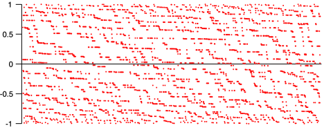
Figure 1: The speed process: simulation of $U_{n}$ for $1\leq n\leq 5000$, from a simulation run to time $700\mbox{,}000$.

a portion of the process. Some aspects of this process were studied in FGM .

1.1 Main results

In order to study the TASEP speed process we prove two results, which are our main tools in understanding the joint distributions of speeds. These results are of significant interest in and of themselves. The following is a new and surprising symmetry of the TASEP. A version of this theorem was proved in DPRW , in the context of the TASEP on finite intervals. We extend it here also to the ASEP (defined in Section 1.3).

Theorem 1.4

Consider the starting configuration $Y_{n}(0)=n$ and $X_{n}(t)$ as above. For any fixed $t>0$ the process $\{X_{n}(t)\}_{n\in\mathbb{Z}}$ has the same distribution as $\{Y_{n}(t)\}_{n\in\mathbb{Z}}$. This holds also for the ASEP.

At any time $t$ we have that $X(t)$ and $Y(t)$ are permutations of $\mathbb{Z}$, one the inverse of the other. Thus this theorem implies that $Y(t)$ as a permutation has the same law as its inverse. It is not hard to see that this holds only for a fixed $t$, and not as processes in $t$ [e.g., $X_{0}(t)$ changes by at most 1 at each jump].

The next result gives additional motivation for considering the speed process, as it relates its law $\mu$ to stationary measures of the multi-type TASEP (and ASEP).

Theorem 1.5

$\mu$ is itself a stationary measure for the TASEP: the unique ergodic stationary measure which has marginals uniform on $[-1,1]$.

This means that if we consider a TASEP in $[-1,1]^{\mathbb{Z}}$ where the initial configuration $Y(0)$ has distribution $\mu$ then at any time $t$ the distribution of $Y(t)$ is also given by $\mu$.

It is known that the $N$-type process has ergodic stationary measures, and that the distribution of $Y_{n}$ among the classes determines this distribution uniquely. Standard techniques (see below) can be used to show that the same holds also with infinitely many classes. Specifically, for any distribution on $\mathbb{R}$ there is a unique ergodic stationary measure for the TASEP with $Y_{0}$ (and any $Y_{n}$) having that distribution. For any two nonatomic distributions on $\mathbb{R}$, these measures are related by applying pointwise a nondecreasing function to the particle classes (see Lemma 5.3), so every such measure can be deduced from the measure with marginals uniform on $[-1,1]$. If a distribution has atoms, then the corresponding stationary measure can still be deduced from the speed process’ law $\mu$ in the same way, but the operation is nonreversible. Thus we have the following characterization:

Corollary 1.6

Every ergodic stationary measure for the TASEP can be deduced from $\mu$ by taking the law of $\{F(U_{n})\}_{n\in\mathbb{Z}}$ for some nondecreasing function $F\dvtx[-1,1]\to\mathbb{R}$.

1.2 Results: Joint distribution

Computer simulations suggested early on that $U_{0},U_{1}$ are not independent (see Figure 2). Recent results of Ferrari, Goncalves and Martin FGM confirm this prediction. They proved (among other things)

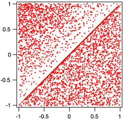
Figure 2: The joint distribution of $U_{0},U_{1}$: based on 5000 pairs from a simulation run to time $25\mbox{,}000$.

that the probability that particle $0$ eventually overtakes particle $1$ (we identify a particle with its class) is $2/3$. It follows that $\mathbb{P}(U_{0}\geq U_{1})\geq 2/3$ (not necessarily equal since $U_{0}=U_{1}$ does not a priori imply overtaking). Our first theorem describing the joint distribution of speeds is the following:

Theorem 1.7

The joint distribution of $(U_{0},U_{1})$, supported on $[-1,1]^{2}$, is

$$f(x,y)\,dx\,dy+g(x)\mathbh{1}(x=y)\,dx$$

with

$$f(x,y)=\cases{\dfrac{1}{4},&\quad$x>y$,\vspace*{2pt}\cr\dfrac{y-x}{4},&\quad$x\leq y$,}\qquad g(x)=\frac{1-x^{2}}{8}.$$

In particular, $\mathbb{P}(U_{0}>U_{1})=1/2$, $\mathbb{P}(U_{0}=U_{1})=1/6$ and $\mathbb{P}(U_{0}<U_{1})=1/3$.

Remarks

Note that the density in $\{U_{0}<U_{1}\}$ (linear in $U_{1}-U_{0}$, so that there is repulsion between the speeds) can be deduced using only Theorem 1.4 (we do not include this argument here). However, proving the—seemingly simpler—constant density on $\{U_{0}>U_{1}\}$ and deriving the singular component on the diagonal requires the power of Theorem 1.5. It is interesting to compare the power of Theorem 1.4 with that of the methods of FGM . It appears that both methods run into similar difficulties and have similar consequences, suggesting a fundamental connection (there are also some parallels in the proofs). Specifically, can the density in the region $\{U_{0}<U_{1}\}$ be derived using the techniques of FMP ? Finally, it is interesting that our proof relies nontrivially on the extension of the TASEP to infinitely many different classes of particles, though the question and answer can both be posed using only $4$ classes (including holes). A similar remark holds about some other results below as well.

Additional information about the joint distribution of speeds is derived in Section 7. We derive certain properties of the $n$-dimensional marginals of $\mu$, and in Theorem 7.7 we compute the joint distribution of three consecutive speeds.

A surprising aspect of Theorem 1.7 is that there is a positive probability ($1/6$) that $U_{0}=U_{1}$, even though each is uniform on $[-1,1]$. Indeed, for any two particles there is a positive probability that their speeds are equal. This phenomenon can be thought of as a spontaneous formation of “convoys,” sets of particles that have the same asymptotic speed, so their trajectories remain close. Our next result gives a full description of such a convoy.

Theorem 1.8

Let the convoy of $0$ be $C_{0}=\{j\dvtx U_{j}=U_{0}\}$, that is, the set of all $j$ with the same speed as $0$. Then $C_{0}$ is $\mu$-a.s. infinite with $0$ density. Moreover, conditioned on $U_{0}$, $C_{0}$ is a renewal process, and the nonnegative elements of $C_{0}$ have the same law as the times of last increase of a random walk conditioned to remain positive, with step distribution

$$\mathbb{P}(X=1)=\mathbb{P}(X=-1)=\frac{1-U_{0}^{2}}{4},\qquad\mathbb{P}(X=0)=\frac{1+U_{0}^{2}}{2}.$$

The “times of last increase” of a walk $Z$ are those indices $n$ for which $m>n$ implies $Z_{m}>Z_{n}$. In particular the convoys are infinite and they provide a translation invariant partition of the integers into infinitely many infinite sets. The convoys are essentially the process with $0$ density for second class particles, seen from a second class particle, as studied by Ferrari, Fontes and Kohayakawa in FFK .

1.3 The ASEP

As the name suggests, the totally asymmetric simple exclusion process is an extremal case of the asymmetric simple exclusion process: the ASEP. The ASEP is defined in terms of a parameter $p\in(1/2,1]$, with $p=1$ being the TASEP. While most quantities involved depend on $p$, the dependence will usually be implicit.

In the ASEP particles jump one site to the right at rate $p\in(1/2,1]$ and to the left at rate ${\overline{p}}=1-p$ (we use the convention ${\overline{x}}=1-x$). The generator of this Markov process is

$$Lf(\eta)=\sum_{n}p\bigl{(}f(\sigma_{n}\eta)-f(\eta)\bigr{)}+{\overline{p}}\bigl{(}f(\sigma_{n}^{*}\eta)-f(\eta)\bigr{)},$$ (3)

where $\sigma_{n}$ and $\sigma_{n}^{*}$ sort the values in $n,n+1$ in decreasing and increasing order, respectively.

While some of the questions above make sense also in this setting, there is a key difficulty in that the analogue of Theorem 1.1 for the ASEP (conjectured below) is still unproved. Using the methods of Ferrari and Kipnis FerrariKipnis it can be proved that $X_{0}(t)/t$ converges in distribution to a random variable uniform in $[-\rho,\rho]$, where hereafter we denote $\rho=2p-1$. Note that the particles in the exclusion process try to perform a random walk with drift $\rho$ (and they cannot go faster than that), that explains why the support of the limiting random variable is changed. In fact, in many ways the ASEP behaves similarly to the TASEP slowed down by a factor of $\rho$.

Conjecture 1.9

In the ASEP, $\lim_{t\to\infty}X_{0}(t)/t$ exists a.s. (and the limit is uniform on $[-\rho,\rho]$).

By the discussion preceding Corollary 1.2 this is equivalent to the following:

Conjecture 1.10

The ASEP speed process measure $\mu^{\mathrm{ASEP}}$ is well defined and translation invariant with each $U_{n}$ uniform on $[-\rho,\rho]$.

In order for statements about the ASEP speed process to make sense we must assume this conjecture, and therefore some of our theorems are conditional on Conjecture 1.9. It should be noted that with minor modifications our results also hold assuming a weaker assumption, namely a joint limit in distribution of the speeds $\{X_{n}(t)/t\}_{n\in\mathbb{Z}}$. In that case, the speed process measure is still defined, even though the particles may not actually have an asymptotic speed.

As noted there, Theorem 1.4 holds also for the ASEP, with no additional condition. Theorem 1.5 becomes conditional:

Theorem 1.11

Assume Conjecture 1.9 holds. Then $\mu^{\mathrm{ASEP}}$ is a stationary measure for the ASEP: the unique ergodic stationary measure which has marginals uniform on $[-\rho,\rho]$.

As in the case of the TASEP, this can be interpreted as follows: if an ASEP is started with initial configuration in $[-\rho,\rho]^{\mathbb{Z}}$ with distribution $\mu^{\mathrm{ASEP}}$, then at any time $t>0$ the distribution of the process is also given by $\mu^{\mathrm{ASEP}}$. Note that both the dynamics and the measure $\mu^{\mathrm{ASEP}}$ depend implicitly on the asymmetry parameter $p$.

A useful tool in studying the speed process is the understanding of the stationary measures of the $N+1$ type TASEP in terms of a multi-line process described below, developed by Angel Angel and Ferrari and Martin FerrariMartin . There is no known analogue for these results that describes the stationary measure of the multi-type ASEP. Thus we need to use other (and weaker) techniques to extract information about the marginals of the ASEP speed process. This explains the contrast in the level of detail between the following results and the corresponding theorems above about the TASEP.

Theorem 1.12

We have the following limit:

$$\lim_{t\to\infty}\mathbb{P}\bigl{(}X_{0}(t)<X_{1}(t)\bigr{)}=\frac{2-p}{3}.$$

Theorem 2.3 of FGM proves that the probability that particles $0$ and $1$ interact at least once (i.e., one of them tries to jump onto the other) is $\frac{1+p}{3p}$. In the next section we will show that this is equivalent to the just stated theorem.

Our next theorem provides information about the joint distribution of $\{U_{0},U_{1}\}$, assuming Conjecture 1.9 holds.

Theorem 1.13

Assume Conjecture 1.9 holds. Let the measure $\mu^{(2)}$ on $[-\rho,\rho]^{2}$ be the marginal of $\{U_{0},U_{1}\}$ under $\mu^{\mathrm{ASEP}}$. Denote by $\tilde{\mu}^{(2)}$ the reflection of $\mu^{(2)}$ about the line $x=y$. Then on $\{(x,y)\dvtx-\rho\leq x<y\leq\rho\}$ we have

$$p\cdot\mu^{(2)}-{\overline{p}}\cdot\tilde{\mu}^{(2)}=\frac{y-x}{4\rho^{2}}\,dx\,dy.$$

We finish this section with a statement concerning the case $U_{0}=U_{1}$. Consider the total amount $J_{i,j}$ of time that particles $i$ and $j$ spend next to each other, that is, $J_{i,j}=\int_{0}^{\infty}\mathbh{1}(|X_{i}(t)-X_{j}(t)|=1)\,dt$.

Theorem 1.14

In the TASEP, $J_{0,1}=\infty$ if and only if $U_{0}=U_{1}$. If Conjecture 1.9 holds, then the same holds for the ASEP.

In the TASEP $J_{0,1}=\infty$ implies that there is at least one interaction between 0 and 1 which means that they are a.s. swapped. (See the next section for a more detailed discussion.) Thus if $U_{0}=U_{1}$, then eventually $X_{0}(t)>X_{1}(t)$. In fact, this holds for any two particles in the same convoy: in Lemma 9.9 we will prove that in the TASEP, particle 0 will eventually overtake all the particles in its convoy with positive index.

1.4 Overview of the paper

The rest of the paper is organized as follows. Section 2 provides some of the background: constructions of the processes and the multi-line description of the stationary measure for the multi-type TASEP. Section 3 includes the proof of the symmetry property (Theorem 1.4) and Section 4 proves the stationarity of the speed process (Theorems 1.5 and 1.11). Sections 6 and 7 include the results about various finite-dimensional marginals of the TASEP speed process. Section 8 deals with the proof of Theorem 1.8. Finally, in Section 9 we prove our results on the ASEP speed process.

2 Preliminaries

2.1 Construction of the process

There are several formal constructions of the TASEP and ASEP. The one that best suits our needs seems to be Harris’s approach Liggett . We include the construction since there are several variations and the exact details are used in some of our proofs. The process is a function $Y$ defined on $\mathbb{Z}\times\mathbb{R}^{+}$. $Y_{k}(t)$ will denote the class of the particle at position $k$ at time $t$. The configuration at time $t$ is $Y(t)=\{Y_{k}(t)\}_{k\in\mathbb{Z}}$. The classes of particles will be real numbers, hence the configuration at any given time is in $\mathbb{R}^{\mathbb{Z}}$. Setting $t=0$ gives the initial configuration $Y(0)$.

We define the transposition operator $\tau_{n}$, acting on $\mathbb{R}^{\mathbb{Z}}$ by exchanging $Y_{n}$ and $Y_{n+1}$, while keeping all other classes equal. Using this we can alternately describe the sorting operator $\sigma_{n}$ by

$$\sigma_{n}Y=\cases{\tau_{n}Y,&\quad$Y_{n}<Y_{n+1}$,\cr Y,&\quad otherwise.}$$

Thus $\sigma_{n}$ has the effect of sorting $Y_{n},Y_{n+1}$ in decreasing order, keeping other classes the same.

The TASEP is defined using the initial configuration and the location of “jump” points. The probability space contains a standard Poisson process on $\mathbb{Z}\times\mathbb{R}^{+}$, that is, a collection of independent standard Poisson processes on $\mathbb{R}^{+}$, denoted $T_{n}$. If $(n,t)$ is a point of $T_{n}$, then at time $t$ the values of $Y_{n}(t^{-})$ and $Y_{n+1}(t^{-})$ may be switched. In the TASEP they are sorted, that is, $Y(t)=Y(t^{-})\cdot\sigma_{n}$. This can be described as applying each of the operators $\sigma_{n}$ at rate 1 independently. A simple percolation argument shows that this dynamic is a.s. well defined. (For any fixed $t>0$ there are a.s. infinitely many integers $n$ so that there are no Poisson points on $\{n\}\times[0,t]$ which means that to define the process up to time $t$ it suffices to consider finite lattices.)

The ASEP

Defining the partially asymmetric exclusion process requires additional randomness. Given the parameter $p\in(1/2,1]$, we attach to each point $(n,t)$ in the Poisson process an independent Bernoulli random variable $X_{n,t}$ with $\mathbb{P}(X_{n,t}=1)=p$. We can now define the probabilistic sorting operator $\rho_{n}$ as follows:

$$\rho_{n}Y=\cases{\sigma_{n}Y,&\quad if $X_{n,t}=1$,\cr\sigma^{*}_{n}Y,&\quad if $X_{n,t}=0$.}$$

Thus with probability $p$ the smaller classed particle is moved to the right position and with probability $1-p$ it is moved to the left position. When such an event happens we say that $Y_{n}(t)$ and $Y_{n+1}(t)$ have an interaction (regardless of whether they were actually swapped). Note that if particles $i,j$ interact in this way, then their order after the swap is independent of the order before the swap. The key observation is that after $i<j$ interact in this way at least once, $i$ has probability $p$ of being to the right of $j$, and this is unchanged by further interactions. Moreover, if we condition on $J_{i,j}(t)=\int_{0}^{\infty}\mathbh{1}(|X_{i}(s)-X_{j}(s)|=1)\,ds$ (the total time $i,j$ spend next to each other until time $t$), then

$$\quad\mathbb{P}\bigl{(}X_{i}(t)<X_{j}(t)|J_{i,j}(t)\bigr{)}=e^{-J_{i,j}(t)}+{\overline{p}}\bigl{(}1-e^{-J_{i,j}(t)}\bigr{)}={\overline{p}}+pe^{-J_{i,j}(t)},$$ (4)

where the expression on the right is just the probability that there were no interaction between $i$ and $j$ until time $t$ plus the probability that there was some interaction, and at time $t$ particle $i$ is to the left of $j$. One of the consequences of (4) is that

$$\lim_{t\to\infty}\mathbb{P}\bigl{(}X_{i}(t)<X_{j}(t)\bigr{)}={\overline{p}}+p\mathbb{E}e^{-J_{i,j}}.$$ (5)

Thus Theorem 1.12 implies ${\overline{p}}+p\mathbb{E}e^{-J}=\frac{2-p}{3}$ which gives $1-\mathbb{E}e^{-J_{0,1}}=\frac{1+p}{3p}$. But $1-\mathbb{E}e^{-J_{0,1}}$ is exactly the probability that there is at least one interaction between $0$ and 1 which shows why Theorem 2.3 of FGM and our Theorem 1.12 are equivalent.

In the TASEP case if there is an interaction between $i<j$, then $X_{i}(t)>X_{j}(t)$ after that. Thus in that case from (5) we get

$$\mathbb{P}\bigl{(}\mbox{eventually }X_{i}(t)>X_{j}(t)|J_{i,j}=\infty\bigr{)}=1,$$

which explains the remark after Theorem 1.14.

There is an alternate construction for the ASEP, which will be used in Section 3. Consider a Poisson process with lower intensity $p$ on $\mathbb{Z}\times\mathbb{R}^{+}$, but whenever it has a point $(n,t)$ we apply at time $t$ the operator $\pi_{n}$ rather then $\rho_{n}$, where $\pi_{n}$ is defined by

$$\pi_{n}Y=\cases{\tau_{n}Y,&\quad$Y_{n}<Y_{n+1}$,\cr\tau_{n}Y,&\quad$Y_{n}>Y_{n+1}$ with prob. $q=(1-p)/p$,\cr Y,&\quad$Y_{n}>Y_{n+1}$ with prob. ${\overline{q}}=(2p-1)/p$.}$$

Thus if the pair is in increasing order it is always swapped, while if it is in decreasing order it is swapped only with probability $q$. It is easy to see that every possible swap occurs at the same rate in the two constructions; hence the resulting processes have the same generator.

2.2 Stationary measures for the multi-type TASEP

The following theorem can be proved by standard coupling methods (see, e.g., Liggettcouple where the same theorem is proved for the 2-type TASEP).

Theorem 2.1

Fix every $0\leq\lambda_{1},\ldots,\lambda_{N}\leq 1$ with $\sum\lambda_{i}=1$. There is a unique ergodic stationary distribution $\nu_{\lambda}$ for the $N$-type TASEP with $\mathbb{P}(Y_{0}=k)=\lambda_{k}$. The measures $\nu_{\lambda}$ are the extremal stationary translation invariant measures. They are the only stationary translation invariant measures with the property that for each $k$, the distribution of $\{\mathbh{1}[Y_{n}\leq k]\}_{n\in\mathbb{Z}}$ is product Bernoulli measure with density $\sum_{j\leq k}\lambda_{j}$.

For the ordinary TASEP (with particles and holes) this stationary distribution is just the product Bernoulli with a fixed density. If we have an $(N+1)$-type TASEP then the structure of the stationary distribution is more complicated. The first description of $\nu_{\lambda}$ for $N=2$ was given by the matrix method DJLS . Reference FFK gave probabilistic interpretations and proofs of the measure and its properties. Recently combinatorial descriptions of $\nu_{\lambda}$ have appeared as well. The $(2+1)$-type TASEP was treated by Angel Angel (see also Duchi–Schaeffer DuchiSchaeffer ). These results were extended for all $N$ by Ferrari and Martin FerrariMartin . They give an elegant construction of $\nu_{\lambda}$ using systems of queues.

We will now briefly describe the $N$-line description of $\nu_{\lambda}$ for the $(N+1)$-type TASEP. The two-line case suffices for most of our results, with the exception of the results of Section 7. For a more detailed description and proofs see FerrariMartin .

From here on we shall fix the parameters $\lambda_{1},\ldots,\lambda_{N+1}$. Consider $N$ independent Bernoulli processes on $\mathbb{Z}$ denoted $\mathbf{B}_{1},\mathbf{B}_{2},\ldots,\mathbf{B}_{N}$ where $\mathbf{B}_{k}$ has parameter $\sum_{i\leq k}\lambda_{i}$ (these are the lines). From these lines we construct a system of $N-1$ coupled queues. The lines give the service time of the queues, and the departures from each queue are the arrivals to the next queue.

It is important to observe that the time for the queues goes from right to left, that is, $\mathbf{B}_{i}(n)$ is followed by $\mathbf{B}_{i}(n-1)$ and so on. The resulting system of queues is positively recurrent, so it can be defined starting at $\infty$ and going over the lines toward $-\infty$.

The $i$th queue will consist of the particles that departed from the $i$th line and are waiting for a service in $\mathbf{B}_{i+1}$. This queue will consist of particles of classes $\{1,\ldots,i\}$. When a service is available in $\mathbf{B}_{i+1}$ the lowest classed particle in the $i$th queue is served and departs (to the next queue). If the queue is empty then a particle of class $i+1$ is said to depart the queue. The departure process of each queue (i.e., the times and sequence of classes of departing customers) is the arrival process for the next queue.

It is convenient to think of an additional queue with $\mathbf{B}_{1}$ as its service times. This queue has no arrivals (so it is always empty). The unused services introduce first class particles, which join the second queue whenever there is a service in $\mathbf{B}_{1}$. These operations are evaluated for each $n$ from line $1$ to line $N$ in order. Let $Q_{i,j}(n)$ be the number of particles of type $j$ in the $i$th queue after column $n$ of the multi-line process has been used.

Note that each queue has a higher rate of service than of arrivals, so the queues sizes are tight, and the state with all queues empty is positively recurrent. In practice, the $i$th queue has $i$ types of particles in it, so the whole system of queues is described by $\frac{N(N-1)}{2}$ nonnegative integers.

Theorem 2.2 ((Ferrari–Martin))

$\nu_{\lambda}$ is the distribution of the departure process of $\mathbf{B}_{N}$, with class $N+1$ (or empty sites) at those $n$ when there is no service.

As an example, and to clarify the graphic representation we use later, consider the following segment of a configuration of the three-line process for $n=\{1,2,3,4\}$. Suppose both queues are empty at time 5. (This is denoted by the $\varnothing,\varnothing$ exponent.) Here, ! denotes a $0$ in the corresponding line, and ” a 1. Later, in cases where we do not care about a specific value we may use $\circledast$ to denote that

$$\framebox{$\begin{array}[c]{*{4}{ @{}c } @{}}{\mbox{\color[rgb]{.5,.5,.5}{{\char 33\relax}}}}&\mbox{{\char 34\relax}}&\mbox{{\char 34\relax}}&{\mbox{\color[rgb]{.5,.5,.5}{{\char 33\relax}}}}\\ \mbox{{\char 34\relax}}&\mbox{\color[rgb]{.5,.5,.5}{{\char 33\relax}}}&\mbox{\color[rgb]{.5,.5,.5}{{\char 33\relax}}}&\mbox{{\char 34\relax}}\\ \mbox{{\char 34\relax}}&\mbox{{\char 34\relax}}&\mbox{\color[rgb]{.5,.5,.5}{{\char 33\relax}}}&\mbox{{\char 34\relax}}\end{array}$}^{\varnothing,\varnothing}.$$

At time $4$, reading the rightmost column from top to bottom, there is no service in $\mathbf{B}_{1}$, so no first class particle joins the second queue, which therefore remains empty. There is a service in $\mathbf{B}_{2}$, and no particles in the first queue, so a second class particle joins the second queue. There is service in $\mathbf{B}_{3}$, so the second class particle departs immediately. Thus at time $4$ the queue states are $(\varnothing,\varnothing)$.

At time $3$ a first class particle arrives to the first queue, and stays there since there is no service in the second queue. There is no further service in column $3$, so the state at time $3$ is $(\{1\},\varnothing)$. There is no departure, which is denoted by a $4$ (or hole). At time $2$ another first class particle arrives, and there is no particle in the second queue so the service in $\mathbf{B}_{3}$ gives rise to a third class particle departing. The states are now $(\{1,1\},\varnothing)$. Finally, at time $1$ a first class particle is served at both $\mathbf{B}_{2}$ and $\mathbf{B}_{3}$, departing and leaving queue states $(\{1\},\varnothing)$. The resulting segment of $\nu_{\lambda}$ is $(1,3,4,2)$.

3 Symmetry

Recall the operators $\pi_{n}$ defined above. These act randomly on configurations, and the ASEP can be defined by applying each of the Markov operators $\pi_{n}$ at rate $p$.

Formally, $\pi_{i}$ is defined as acting on $\mathcal{M}(S_{\infty})$: probability measures on $S_{\infty}$. Given a measure $\nu$ on $S_{\infty}$, we let $\pi_{n}\nu$ be the distribution of $\pi_{n}$ applied to a sample from $\nu$. Since $\tau_{i}$ and $\sigma_{i}$ also act naturally on the measures (in the same way), one finds the operator relation

$$\pi_{i}=q\tau_{i}+{{\overline{q}}}\sigma_{i}.$$

Note that $p=1$ gives $q=0$ so in that case $\pi_{i}=\sigma_{i}$. In the case $p=1/2$ we get $q=1$ and $\pi_{i}=\tau_{i}$, so the process reduces to a symmetric random walk on $S_{\infty}$.

The crucial observation leading to Theorem 1.4 is the following lemma.

Lemma 3.1

Fix any $p\geq 1/2$, and sequence $i_{1},\ldots,i_{n}$. Then

$$\pi_{i_{n}}\cdots\pi_{i_{1}}\cdot\operatorname{id}\stackrel{{\scriptstyle d}}{{=}}(\pi_{i_{1}}\cdots\pi_{i_{n}}\cdot\operatorname{id})^{-1}.$$ (6)

That is, applying a sequence of $\pi_{i}$’s in the reverse order to the identity leads to the inverse permutation. This is trivially true when $p=1/2$ and $\pi=\tau$, but requires proof for other $p$. When $p\in\{1/2,1\}$ the operator is deterministic and this distributional identity is an equality of permutations. Proof of Theorem 1.4 The theorem follows from Lemma 3.1 since at any finite time at each $i$ there is positive probability ($e^{-t}$) that no swap has occurred. Each such $i$ separates $\mathbb{Z}$ into two parts with independent behavior, so the state of the process is a product of finite, mutually commuting permutations. The distribution of the sequence of applied operators between such inactive locations is symmetric in time.

We now prove Lemma 3.1. In the case of the TASEP, Lemma 3.1 and Theorem 1.4 were first proved in DPRW . To prove the lemma in the general case, we start with the following facts about the transposition operators. The identities are readily verified, and the last claim is known as Matsumoto’s lemma (see, e.g., coxetergroups , Theorem 3.3.1).

Fact 3.2.

The operators $\tau_{i}$ satisfy the relations

$$\tau_{i}^{2} = I,$$ (7)

$$\tau_{i}\tau_{j} = \tau_{j}\tau_{i}\qquad\mbox{for }|i-j|>1,$$ (8)

$$\tau_{i}\tau_{i+1}\tau_{i} = \tau_{i+1}\tau_{i}\tau_{i+1},$$ (9)

where $I$ denotes the identity operator. With these relations the operators $\{\tau_{i}\}$ generate the symmetric group. Furthermore, it is possible to pass between any two minimal words of the same permutation (i.e., words of minimal length representing that permutation) using only relations (8), (9).

The $\pi$’s satisfy similar relations:

Lemma 3.3

The operators $\{\pi_{i}\}$ satisfy the relations

$$\pi_{i}^{2} = qI+{\overline{q}}\pi_{i},$$ (10)

$$\pi_{i}\pi_{j} = \pi_{j}\pi_{i}\qquad\mbox{for }|i-j|>1,$$ (11)

$$\pi_{i}\pi_{i+1}\pi_{i} = \pi_{i+1}\pi_{i}\pi_{i+1}.$$ (12)

Note that only the first relation differs from the corresponding relation for $\tau$. When $p=1/2$ these reduce to the relations for $\tau$. In the case $p=1$ the first relation becomes $\sigma_{i}^{2}=\sigma_{i}$. In that case, the only nontrivial relation is (12) which is true since both sides have the effect of sorting the three terms involved in decreasing order. Proof of Lemma 3.3 Equation (10) is easy to check, and (11) is trivial. For (12), using $\pi=q\tau+{\overline{q}}\sigma$ and expanding, we need to show that

$$q^{3}(\tau_{i}\tau_{i+1}\tau_{i})+q^{2}{\overline{q}}(\tau_{i}\tau_{i+1}\sigma_{i}+\tau_{i}\sigma_{i+1}\tau_{i}+\sigma_{i}\tau_{i+1}\tau_{i})$$

$$\qquad{}+q{\overline{q}}^{2}(\tau_{i}\sigma_{i+1}\sigma_{i}+\sigma_{i}\tau_{i+1}\sigma_{i}+\sigma_{i}\sigma_{i+1}\tau_{i})+{\overline{q}}^{3}(\sigma_{i}\sigma_{i+1}\sigma_{i})$$

is unchanged by exchanging $i$ and $i+1$. It is easy to verify that

$$\tau_{i}\tau_{i+1}\tau_{i} = \tau_{i+1}\tau_{i}\tau_{i+1},\qquad\tau_{i}\tau_{i+1}\sigma_{i}=\sigma_{i+1}\tau_{i}\tau_{i+1},\qquad\tau_{i}\sigma_{i+1}\tau_{i}=\tau_{i+1}\sigma_{i}\tau_{i+1},$$

$$\sigma_{i}\sigma_{i+1}\sigma_{i} = \sigma_{i+1}\sigma_{i}\sigma_{i+1},\qquad\sigma_{i}\tau_{i+1}\tau_{i}=\tau_{i+1}\tau_{i}\sigma_{i+1},$$

so it remains to show

$$\tau_{i}\sigma_{i+1}\sigma_{i}+\sigma_{i}\tau_{i+1}\sigma_{i}+\sigma_{i}\sigma_{i+1}\tau_{i}=\tau_{i+1}\sigma_{i}\sigma_{i+1}+\sigma_{i+1}\tau_{i}\sigma_{i+1}+\sigma_{i+1}\sigma_{i}\tau_{i+1}.$$

We may assume $i=0$. Since only the relative order of $\eta_{0},\eta_{1},\eta_{2}$ matters, we may assume these are $\{0,1,2\}$ in some order. Applying these operators to the $6$ possible orders gives Table 1.

=240pt $\bolds{\eta}$ 012 021 102 120 201 210 $\tau_{0}\sigma_{1}\sigma_{0}\cdot\eta$ 210 120 210 120 120 120 $\sigma_{0}\sigma_{1}\tau_{0}\cdot\eta$ 210 210 201 210 201 210 $\sigma_{0}\tau_{1}\sigma_{0}\cdot\eta$ 210 210 210 201 210 201 $\tau_{1}\sigma_{0}\sigma_{1}\cdot\eta$ 210 210 201 201 201 201 $\sigma_{1}\sigma_{0}\tau_{1}\cdot\eta$ 210 120 210 120 210 210 $\sigma_{1}\tau_{0}\sigma_{1}\cdot\eta$ 210 210 210 210 120 120

Table 1: See proof of Lemma 3.3

In each column, the entries in the top half are a permutation of the entries in the bottom half, so adding the first three operators gives the same result as adding the last three. Proof of Lemma 3.1 Given $(i_{1},\ldots,i_{n})$, let $X=\tau_{i_{1}}\cdots\tau_{i_{n}}$. If this is a minimal (w.r.t. length) word for $X$ in $S_{\infty}$, then $\pi_{i_{n}}\cdots\pi_{i_{1}}\cdot\operatorname{id}=X$ with probability 1. In this case, the reverse word is minimal for $X^{-1}$, so the claim holds.

The proof proceeds by induction on $n$. Take some sequence $(i_{1},\ldots,i_{n})$. If the representation $\tau_{i_{1}}\cdots\tau_{i_{n}}$ is minimal, then the claimed identity holds. Otherwise, let $k$ be maximal such that $X=\tau_{i_{1}}\cdots\tau_{i_{k}}$ is a minimal representation. By maximality of $k$ we see that $Y=X\tau_{i_{k+1}}$ has a shorter representation, so there is a representation $Y=\tau_{j_{1}}\cdots\tau_{j_{k-1}}$. (The length is $k-1$ and not $k$ since its parity is opposite that of $X$.) Thus $X=\tau_{j_{1}}\cdots\tau_{j_{k-1}}\tau_{i_{k+1}}$ is another minimal representation of $X$.

Starting with $\pi_{i_{1}}\cdots\pi_{i_{n}}$, we can repeatedly apply relations (11) and (12) to the first $k$ terms in the product, to get

$$\pi_{i_{1}}\cdots\pi_{i_{n}}=\pi_{j_{1}}\cdots\pi_{j_{k-1}}\pi_{i_{k+1}}^{2}\cdots\pi_{i_{n}}.$$

Here $i_{k+1}^{2}$ appears twice since it is both the last term in the alternate representation of $X$ and the first in the remainder of the sequence. Relation (10) now gives

$$\quad\pi_{i_{1}}\cdots\pi_{i_{n}}=q(\pi_{j_{1}}\cdots\pi_{j_{k-1}}\pi_{i_{k+2}}\cdots\pi_{i_{n}})+{\overline{q}}(\pi_{j_{1}}\cdots\pi_{j_{k-1}}\pi_{i_{k+1}}\cdots\pi_{i_{n}}).$$ (13)

Similarly, working with the reverse sequence,

$$\quad\pi_{i_{n}}\cdots\pi_{i_{1}}=q(\pi_{i_{n}}\cdots\pi_{i_{k+2}}\pi_{j_{k-1}}\cdots\pi_{j_{1}})+{\overline{q}}(\pi_{i_{n}}\cdots\pi_{i_{k+1}}\pi_{j_{k-1}}\cdots\pi_{j_{1}}).$$ (14)

Applying (14) and (13) to to $\operatorname{id}$, and using the induction hypothesis for the shorter sequences $(j_{1},\ldots,j_{k-1},i_{k+1},\ldots,i_{n})$ and $(j_{1},\ldots,j_{k-1},i_{k+2},\ldots,i_{n})$ completes the proof.

Note: the proof actually shows that any word in the $\pi$’s can be reduced (as an operator) to some convex combination of words corresponding to minimal words.

Corollary 3.4

Consider the infinite type TASEP with initial condition $Y_{n}(0)=n$. Then $\{\frac{Y_{n}(t)}{t}\}_{n\in\mathbb{Z}}$ converges weakly to $\mu$ as $t\to\infty$.

For any $t$ this process has the same law as $\{\frac{X_{n}(t)}{t}\}_{n\in\mathbb{Z}}$, which converges a.s. to a process with law $\mu$.

4 Stationarity

We will give two different proofs of the stationarity of the distribution of the speed process. The first is specific to the TASEP, and is reminiscent of coupling from the past. It uses the Harris construction directly. The second proof is based on the symmetry between $\{X_{n}(t)\}$ and $\{Y_{n}(t)\}$ (or more specifically Corollary 3.4). The second proof holds also for the ASEP, word by word, under the assumption that Corollary 3.4 is true for the ASEP (which is weaker then Conjecture 1.9).

4.1 Coupling proof

Lemma 4.1

Consider two TASEPs $Y,Y^{\prime}$ defined via the Harris construction as the function of the same Poisson process on $\mathbb{Z}\times\mathbb{R}^{+}$. We set the initial conditions as $Y_{n}(0)=n$ and $Y^{\prime}(0)=\sigma_{0}Y(0)$ (i.e., particles 0 and 1 are switched initially in $Y^{\prime}$). Let $\{U_{n}\}=\{\lim_{t\to\infty}X_{n}(t)/t\}$ denote the speed process of $Y$, and $\{U^{\prime}_{n}\}=\{\lim_{t\to\infty}X^{\prime}_{n}(t)/t\}$ denote the speed process of $Y^{\prime}$. Then $U^{\prime}=\sigma_{0}U$.

All particles other than $\{0,1\}$ are either larger or smaller than both $0$ and $1$, so any swaps involving a particle other than $\{0,1\}$ will occur or not occur equally in $Y$ and $Y^{\prime}$. It follows that for any $i\notin\{0,1\}$ we have $X_{i}(t)=X^{\prime}_{i}(t)$ and hence $U_{i}=U^{\prime}_{i}$. Similarly, since 0 and 1 must fill the only vacant trajectories, $\{U_{0},U_{1}\}=\{U^{\prime}_{0},U^{\prime}_{1}\}$ as an unordered pair.

In $Y^{\prime}$ particle $0$ is always to the right of particle $1$, so $U^{\prime}_{0}=\max\{U_{0},U_{1}\}$ and $U^{\prime}_{1}=\min\{U_{0},U_{1}\}$, completing the proof. Proof of Theorem 1.5 using coupling Consider a Poisson process on $\mathbb{Z}\times\mathbb{R}$. Half of the process, namely the restriction to $\mathbb{Z}\times\mathbb{R}^{+}$ is used in the Harris construction of the TASEP. Similarly, for any $s\in\mathbb{R}$ we can translate the Poisson process by $s$ [i.e., take all points of the form $(n,t+s)$ where $(n,t)$ is in the original process], and take the restriction to $\mathbb{Z}\times\mathbb{R}^{+}$, which can be used in the Harris construction to get a different (though highly dependent) instance of the TASEP.

Let $U_{n}(s)$ be the speed process resulting from the Harris construction using the translated Poisson process. Clearly for every $s$, $U(s)$ has the same law $\mu$, so we are done if we show that $U_{n}(s)$ evolves as a TASEP (with time parameter $s$). Consider the effect of an infinitesimal positive shift $s$. The shift adds new $\sigma$ operations, to be applied before the original sequence of operations. These are added at rate 1 at each location. By the previous lemma, the effect on the resulting speeds of applying $\sigma_{n}$ before using the same Poisson process is to apply $\sigma_{n}$ to the speeds, which is exactly what we need.

It is interesting to note that in the Poisson process $\mathbb{Z}\times\mathbb{R}$, the part on $\mathbb{Z}\times\mathbb{R}^{+}$ is used to determine the “initial” speed process $U(0)$, and the restriction to $\mathbb{Z}\times\mathbb{R}^{-}$ is used exactly as in the Harris construction to generate the TASEP dynamics of $U(s)$.

4.2 Symmetry based proof

Proof of Theorems 1.5 and 1.11 using symmetry We write the proof for $\mu$, but it holds verbatim for $\mu^{\mathrm{ASEP}}$ under Conjecture 1.9.

Informally, we argue as follows. Fix $s$ and let $t\to\infty$. Both $\frac{X_{t}}{t}$ and $\frac{X_{t+s}}{t+s}$ converge a.s. to a sample of $\mu$. By Theorem 1.4 these have the same law as $\frac{Y_{t}}{t}$ and $\frac{Y_{t+s}}{t+s}$, so for large $t$ both of these have law close to $\mu$. However, the result of letting $\frac{Y_{t}}{t}$ evolve for an additional $s$ time is $\frac{Y_{t+s}}{t}$, which is close to $\frac{Y_{t+s}}{t+s}$.

Let $P_{s}$ be the evolution operator for the Markov process corresponding to the generator $L$ on $\mathbb{R}^{\mathbb{Z}}$ [see (1)]. To prove stationarity it is enough to show that for every $0<s$ and every bounded continuous local function $f\dvtx\mathbb{R}^{\mathbb{Z}}\to\mathbb{R}$ we have

$$\int P_{s}f(\eta)\,d\mu(\eta)=\int f(\eta)\,d\mu(\eta).$$ (15)

Consider the process $\{Y_{n}(t)\}_{n\in\mathbb{Z}}$ started from $Y_{n}(0)=n$ and denote the distribution of $\{\frac{Y_{n}(t)}{t}\}_{n}$ by $\nu_{t}$. By Corollary 3.4 the weak limit of $\nu_{t}$ is $\mu$ which means that for every local bounded continuous function $f\dvtx\mathbb{R}^{\mathbb{Z}}\to\mathbb{R}$ we have

$$\int f(\eta)\,d\nu_{t}(\eta)\mathop{\longrightarrow}\limits_{t\to\infty}\int f(\eta)\,d\mu(\eta).$$

For any fixed $s$

$$\int P_{s}f(\eta)\,d\nu_{t}(\eta)\mathop{\longrightarrow}\limits_{t\to\infty}\int P_{s}f(\eta)\,d\mu(\eta).$$

But $\int P_{s}f(\eta)\,d\nu_{t}(\eta)=\int f(\frac{t+s}{t}\eta)\,d\nu_{t+s}(\eta)$ which (for any fixed $s$, as $t\to\infty$) converges to $\int f(\eta)\,d\mu(\eta)$. Now (15) and the theorem follow.

5 Basic properties of stationary distributions

In this section we present a medley of simple results concerning the (T)ASEP and its stationary distributions. These are only weakly related to each other, and are collected here for convenience.

Proposition 5.1

$\mu$ is ergodic for the shift. Under Conjecture 1.9, so is $\mu^{\mathrm{ASEP}}$.

Consider the setup of Corollary 1.2 and use the Harris construction with independent standard Poisson processes $T_{n}$ on the interval $[0,\infty)$ to define $y_{n}(t)$ and the variables $X_{n}(t)$. Then the limit process $\{U_{n}\}_{n\in\mathbb{Z}}$ is measurable with respect to the $\sigma$-algebra $\mathcal{F}$ generated by the i.i.d. processes $T_{n}$ ($n\in\mathbb{Z}$). Since $\mathcal{F}$ is generated by i.i.d. processes any translation invariant event in $\mathcal{F}$ has to be trivial. But then the same thing must be true for any translation invariant event in the $\sigma$-algebra generated by $\{U_{n}\}_{n\in\mathbb{Z}}$ as this is a sub-$\sigma$-algebra of $\mathcal{F}$.

There are three possible “reflections” for the ASEP. One may reverse the direction of space, so that (low classed) particles flow to the left and not right; one can consider the time reversal of the dynamics, and one can reverse the order of classes (or keep the same generator but replace class $k$ with $-k$, or $N+1-k$, etc.). It is easy to see that reversal of both space and class order preserves the original dynamics. This is called the space-class symmetry of the TASEP/ASEP.

The following proposition is the space-class symmetry of the speed process, and follows directly from the corresponding symmetry of the ASEP process.

Proposition 5.2

For the TASEP $\{U_{n}\}_{n\in\mathbb{Z}}\stackrel{{\scriptstyle d}}{{=}}\{-U_{-n}\}_{n\in\mathbb{Z}}$. This also holds for the ASEP, assuming Conjecture 1.9 holds.

The following observation and its corollary provide an important connection between the distribution of the speed process and the stationary measures of multi-type ASEP. These connections will be used to extract information on the joint distribution of the speeds of several particles in Sections 6 and 7.

Lemma 5.3

Let $\{\eta_{n}(t)\}_{n,t}$ be an ASEP, and let $F\dvtx\mathbb{R}\rightarrow\mathbb{R}$ be a nondecreasing function. Then $\{F(\eta_{n}(t))\}_{n,t}$ is also an ASEP (with the same asymmetry parameter).

The ASEP is defined as applying to $\eta(t)$ each of the operators $\pi_{n}$ independently at rate $1$. Applying a nondecreasing function to each coordinate commutes with every $\pi_{i}$, hence $\{F(\eta_{n}(t))\}_{n,t}$ is just the ASEP with initial configuration $\{F(\eta_{n}(0)\}_{n}$.

Corollary 5.4

If $F\dvtx[-1,1]\rightarrow\{1,\ldots,N\}$ is nondecreasing, then for the TASEP the distribution of $\{F(U_{n})\}$ is the unique ergodic stationary measure of the multi-type TASEP with types $\{1,\ldots,N\}$ and densities $\lambda_{i}=\frac{1}{2}\operatorname{{\mathfrak{L}eb}}(F^{-1}(i))$.

This also holds for the ASEP (and its corresponding multi-type stationary measure) under Conjecture 1.9.

Let $\mu_{F}$ denote the distribution of $\{F(U_{n})\}$. Since $\mu$ is ergodic, so is $\mu_{F}$. The marginals are as claimed since each $U_{n}$ is uniform on $[-1,1]$.

To prove that $\mu_{F}$ is stationary, start a TASEP $Y_{n}(t)$ with initial configuration $Y_{n}(0)=U_{n}$. By Lemma 5.3 $\{F(Y_{n}(t))\}_{n,t}$ is a $N$-type TASEP. Since $\mu$ is stationary, $Y(t)$ also has law $\mu$, and so $\{F(Y_{n}(t))\}_{n,t}\stackrel{{\scriptstyle d}}{{=}}\{F(Y_{n}(0))\}_{n,t}$, hence $\mu_{F}$ is also stationary.

The result for the ASEP follows the same way.

The next proposition shows that a TASEP started with uniform i.i.d. classes must converge to the speed process. In particular, even though classes in the i.i.d. initial distribution are a.s. all different, the process converges to the speed process which has infinite convoys of particles with the same class (see Section 8). Thus the TASEP dynamics has the effect of aggregating particles with increasingly closer speeds next to each other.

Proposition 5.5

Consider a TASEP where $Y_{n}(0)$ are i.i.d. uniform on $[-1,1]$. Then $\{Y_{n}(t)\}_{n\in\mathbb{Z}}$ converges weakly to $\mu$. The same holds for the ASEP under Conjecture 1.9

Let $\nu_{t}$ be the distribution of $Y(t)$ for the process $Y$ of the lemma. We need to show that $\int g\,d\nu_{t}\mathop{\longrightarrow}\limits_{t\to\infty}\int g\,d\mu$ for any fixed bounded and continuous function $g\dvtx[-1,1]^{\mathbb{Z}}\to\mathbb{R}$.

If we start the $N$-type TASEP with an i.i.d. product measure initial distribution then its distribution converges to an ergodic stationary measure with the same one-dimensional marginal. (This can be shown by standard coupling arguments introduced by Liggett; see, e.g., Liggettcouple or Liggett , Chapter 8.)

Using Lemma 5.3 and Corollary 1.6 it follows that for any nondecreasing step function $F$ on $[-1,1]$ the process $\{F(Y_{n}(t))\}_{n}$ converges in distribution to $\{F(U_{n})\}_{n}$.

For an integer $M$ let $F_{M}(x)=\frac{\lfloor Mx\rfloor}{M}$, which maps $[-1,1]$ to $\{i/M,i\in[-M$, $M-1]\}$. Define the operator $F^{\otimes}_{M}$ on configurations, as the operator that applies $F_{M}$ to each coordinate: $F^{\otimes}_{M}(\eta)_{n}=F_{M}(\eta_{n})$. Since $g$ is continuous we can select $M$ such that $\|g-g\circ F^{\otimes}_{M}\|_{\infty}\leq\varepsilon$. By the triangle inequality we have

$$\biggl{|}\int g\,d\nu_{t}-\int g\,d\mu\biggr{|}\leq 2\varepsilon+\biggl{|}\int g\circ F^{\otimes}_{M}\,d\nu_{t}-\int g\circ F^{\otimes}_{M}\,d\mu\biggr{|},$$

and $g\circ F^{\otimes}_{M}$ is $g$ applied to a TASEP with finitely many types, so it can be made smaller than $\varepsilon$ by taking $t$ large enough.

6 Two-dimensional marginals of the TASEP speed process

The key tool for analyzing the joint densities of the speed process is Corollary 5.4. This states that if the speed process is monotonously projected into $\{1,\ldots,k,\break k+1\}$, then the result is the stationary measure of the multi-type TASEP with suitable densities. In the TASEP, the latter is given in terms of the multi-line process (see Section 2.2). More explicitly, we will use the following projections, to which we refer as canonical projections. Let $\mathbf{x}=(x_{1},\ldots,x_{k})$ be an increasing sequence taking values in $[0,1]$, with the conventions that $x_{0}=0$ and $x_{k+1}=1$. Define $F\dvtx[-1,1]\to\{1,\ldots,k,k+1\}$ by

$$F(u)=F_{\mathbf{x}}(u)=\min\{i\dvtx\hat{u}<x_{i}\}\qquad\mbox{where }\hat{u}=\frac{1+u}{2}.$$

Note that if $u$ is uniform on $[-1,1]$, then $F(u)=i$ with probability $x_{i}-x_{i-1}$. Let $V_{i}=F(U_{i})$, so each $V_{i}$ has distribution controlled by the $x$’s. It is not hard to see that the $\sigma$-field generated by $V_{1},\ldots,V_{k}$ (or any $k$ fixed indices) for all possible $\mathbf{x}$’s is the same as the $\sigma$-field of $U_{1},\ldots,U_{k}$.

The scheme of our argument should now be clear. The distribution of $V$ is given by a multi-line process, and can be computed explicitly. Considering the resulting probabilities as functions of $\mathbf{x}$ allows us to recover the joint density of the corresponding speeds. This last step is done by taking suitable derivatives w.r.t. $x_{i}$’s to get the density. In order to find the joint density of $k$ particles we work with the $k$-line process. In this section we use this approach to prove results about two-dimensional marginals of $\mu$. We prove Theorem 1.7 which gives the joint distribution of $(U_{0},U_{1})$ and generalize this result for the joint distribution of any two speeds. In the next section we give some results for higher-dimensional marginals.

6.1 Two consecutive speeds: $U_{0},U_{1}$

Proof of Theorem 1.7 We compute the probability that $V_{1}=2$ and $V_{0}$ is each of $1,2,3$ (recall that as the highest class particles, $3$’s are equivalent to holes). The queue of the two line process is a single, simple queue, so indices are not needed. In order to have a second class particle at position $1$ we need an unused service. This means the queue must be empty: $Q(2)=0$, and there must be a particle at the bottom line but not at the top line in position $1$. The intersection of these events has probability $x_{2}-x_{1}$ (as this is the density of second class particles). More importantly, they depend only on the two-line configuration in positions $\{1,\ldots,\infty\}$. Since on this event the queue is also empty at position 1, the class $V_{0}$ depends only on the two-line configuration at position 0.

In particular, to get a first class particle, $V_{0}=1$, the only possibility is to also have particles in both lines in position 0. This leads to

$$\mathbb{P}(V_{0}=1,V_{1}=2)=\mathbb{P}\biggl{(}\framebox{$\begin{array}[c]{*{2}{ @{}c } @{}}\mbox{{\char 34\relax}}&\mbox{\color[rgb]{.5,.5,.5}{{\char 33\relax}}}\\ \mbox{{\char 34\relax}}&\mbox{{\char 34\relax}}\end{array}$}^{\varnothing}\biggr{)}=x_{1}x_{2}(x_{2}-x_{1}).$$

We shall also denote this probability by $\mu_{\mathbf{x}}(1,2)$ for compactness, as this is the probability of seeing consecutive particles of classes $1,2$ in the stationary measure $\mu_{\mathbf{x}}$. Similarly we have

$$\mu_{\mathbf{x}}(2,2) = \mathbb{P}\biggl{(}\framebox{$\begin{array}[c]{*{2}{ @{}c } @{}}\mbox{\color[rgb]{.5,.5,.5}{{\char 33\relax}}}&\mbox{\color[rgb]{.5,.5,.5}{{\char 33\relax}}}\\ \mbox{{\char 34\relax}}&\mbox{{\char 34\relax}}\end{array}$}^{\varnothing}\biggr{)}=x_{1}{\overline{x}}_{2}(x_{2}-x_{1}),$$

$$\mu_{\mathbf{x}}(3,2) = \mathbb{P}\biggl{(}\framebox{$\begin{array}[c]{*{2}{ @{}c } @{}}\raisebox{0.9pt}{\mbox{{$\circledast$}}}&\mbox{\color[rgb]{.5,.5,.5}{{\char 33\relax}}}\\ \mbox{\color[rgb]{.5,.5,.5}{{\char 33\relax}}}&\mbox{{\char 34\relax}}\end{array}$}^{\varnothing}\biggr{)}={\overline{x}}_{1}(x_{2}-x_{1}).$$

Here, $\circledast$ indicates no restriction on the top line in that position and ${\overline{y}}=1-y$.

To calculate the densities of the two speeds we find, for example,

$$\mathbb{P}(U_{0}<2x_{1}-1<U_{1}<2x_{2}-1)=\mu_{\mathbf{x}}(1,2)=x_{1}x_{2}(x_{2}-x_{1}).$$

Thus to find the density at $(u_{0},u_{1})$ for $u_{0}<u_{1}$ we need to take derivatives w.r.t. $x_{2}$ and $x_{1}$, and set $x_{2}=(1+u_{1})/2$, $x_{1}=(1+u_{0})/2$. Remembering the Jacobians ($1/2$) we find

$$\mathbb{P}(U_{0}\in du_{0},U_{1}\in du_{1})=\biggl{(}\frac{1}{2}\,\partial_{x_{1}}\biggr{)}\biggl{(}\frac{1}{2}\,\partial_{x_{2}}\biggr{)}\mu_{\mathbf{x}}(1,2)=\frac{u_{1}-u_{0}}{4}\,du_{0}\,du_{1}$$ (18)

$$\eqntext{\mbox{for $u_{0}<u_{1}$.}}$$

Similarly, to find the density at $(u_{0},u_{1})$ for $u_{0}>u_{1}$ noting that the Jacobians now have reversed signs we find

$$\mathbb{P}(U_{0}\in du_{0},U_{1}\in du_{1})=\biggl{(}-\frac{1}{2}\,\partial_{x_{1}}\biggr{)}\biggl{(}-\frac{1}{2}\,\partial_{x_{2}}\biggr{)}\mu_{\mathbf{x}}(3,2)=\frac{1}{4}\,du_{0}\,du_{1}$$ (19)

$$\eqntext{\mbox{for $u_{0}>u_{1}$.}}$$

Finally, to find the (singular) density along the diagonal, consider $\mu_{\mathbf{x}}(2,2)$ and let $x_{2},x_{1}\to\frac{1+u}{2}$. We have

$$\mathbb{P}(U_{0},U_{1}\in du)=\frac{1}{2}\lim_{x_{1},x_{2}\to(1+u)/2}\frac{\mu_{\mathbf{x}}(2,2)}{x_{2}-x_{1}}=\frac{1-u^{2}}{8}\,du.$$

6.2 Two distant speeds: $U_{0},U_{k}$

The two line process also yields formulae for the joint density of two distant particles. However, the result is not as compact as for the case of two consecutive particles.

Theorem 6.1

For any $k>0$ we have:

• The joint density of $U_{0},U_{k}$ on $\{U_{0}>U_{k}\}$ is $1/4$ [so $\mathbb{P}(U_{0}>U_{k})=1/2$].

• On $\{U_{0}<U_{k}\}$ the density is a polynomial of degree $2k-1$.

• On the diagonal $\{U_{0}=U_{k}\}$ the density is a polynomial of degree $2k$. As $k\to\infty$, the density on the diagonal $\{(u,u)\dvtx|u|\leq 1\}$ is asymptotically $\sqrt{\frac{1-u^{2}}{16\pi k}}$.

It is possible to prove exponential convergence of the density on $\{U_{0}<U_{k}\}$ to $1/4$, though we do not pursue that direction here. The fact that as $k\to\infty$ the distributions of $U_{0}$ and $U_{k}$ become independent follows from ergodicity, or can be read from (22) below.

The theorem follows easily from the next two lemmas. Let $\{S_{n}\}$ be a random walk with steps in $\{1,-1,0\}$ with probabilities $\{p_{+},p_{-},p_{0}\}$, and consider the maximum process $M_{n}=\max_{i\leq n}S_{i}$.

Lemma 6.2

Fix $0\leq x<y\leq 1$, and let $S_{n},M_{n}$ be as above with

$$p_{+}=x{\overline{y}},\qquad p_{-}={\overline{x}}y,\qquad p_{0}=xy+{\overline{x}}\,{\overline{y}}.$$

Then we have the following:

$$\mathbb{P}(x<\hat{U}_{k}<y<\hat{U}_{0}) = (y-x){\overline{y}},$$ (20)

$$\mathbb{P}(\hat{U}_{0},\hat{U}_{k}\in[x,y]) = (y-x){\overline{x}}y\mathbb{P}(M_{k-1}=0),$$ (21)

$$\mathbb{P}(\hat{U}_{0}<x<\hat{U}_{k}<y) = (y-x)xy+(y-x){\overline{x}}y\mathbb{P}(M_{k-1}>0).$$ (22)

Note that the steps of $S$ are the difference of two Bernoulli random variables, and therefore $S_{j}\stackrel{{\scriptstyle\mathrm{d}}}{{=}}\operatorname{Bin}(j,x)-\operatorname{Bin}(j,y)$. In particular, for any fixed $x<y$ we have $S_{j}\mathop{\longrightarrow}\limits_{j\to\infty}\limits^{\mathrm{prob}.}-\infty$, and asymptotically the speeds are independent. Proof of Lemma 6.2 By Corollary 5.4, $\mathbb{P}(x<\hat{U}_{k}<y<\hat{U}_{0})=\mu_{x,y}(3,2)$ (where $\mu_{x,y}$ the extremal stationary $3$ type TASEP with densities $x,y-x,\break 1-y$). Using the two-line description of $\mu_{x,y}$ we have $V_{0}=1,V_{k}=2$ if and only if we see the two-line configuration

$$\framebox{$\begin{array}[c]{*{3}{ @{}c } @{}}\raisebox{0.9pt}{\mbox{{$\circledast$}}}&\cdots&\mbox{\color[rgb]{.5,.5,.5}{{\char 33\relax}}}\\ \mbox{\color[rgb]{.5,.5,.5}{{\char 33\relax}}}&\cdots&\mbox{{\char 34\relax}}\end{array}$}^{\varnothing}.$$

Having the hole in the bottom line at position 0 has probability ${\overline{y}}$ and this is independent of having a second class particle at position $k$.

Similarly, to have $\hat{U}_{0},\hat{U}_{k}\in[x,y]$ we need the configuration

$$\framebox{$\begin{array}[c]{*{3}{ @{}c } @{}}\mbox{\color[rgb]{.5,.5,.5}{{\char 33\relax}}}&\cdots&\mbox{\color[rgb]{.5,.5,.5}{{\char 33\relax}}}\\ \mbox{{\char 34\relax}}&\cdots&\mbox{{\char 34\relax}}\end{array}$}^{\varnothing}$$

with intermediate configuration leaving the queue empty at position 1. Let $S_{j}$ be the number of particles in the top line in positions $\{1,\ldots,j\}$ minus the number of particles in the bottom line in those positions. The condition that the queue ends up nonempty is equivalent to $\{\max_{0<j<k-1}S_{j}\geq 1\}$. The claim follows.

Finally, the third case follows from the first two since the three probabilities must add up to $\mathbb{P}(\hat{U}_{k}\in[x,y])=y-x$.

Lemma 6.3

Let $S_{n},M_{n}$ be as above with $p_{+}=p_{-}$. Then $\mathbb{P}(M_{n}=0)=\mathbb{P}(S_{n}\in\{0,-1\})$.

Reflection at the hitting time of $1$ shows that

$$\mathbb{P}(M_{n}>0,S_{n}\leq 0)=\mathbb{P}(M_{n}>0,S_{n}\geq 2)=\mathbb{P}(S_{n}\geq 2)=\mathbb{P}(S_{n}\leq-2).$$

It follows that

$$\mathbb{P}(M_{n}>0)=\mathbb{P}(S_{n}>0)+\mathbb{P}(M_{n}>0,S_{n}\leq 0)=1-\mathbb{P}(S_{n}\in\{0,-1\}).$$

Proof of Theorem 6.1 The case $U_{0}>U_{k}$ is just the double derivative of (20).

For the case $U_{0}=U_{k}$, note from (21) that the density along the diagonal is

$$\lim_{x,y\to\hat{u}}\frac{\mathbb{P}(\hat{U}_{0},\hat{U}_{k}\in[x,y])}{2(y-x)}=\frac{1-u^{2}}{8}\mathbb{P}(M_{k-1}=0),$$

where $M_{k-1}$ is the maximum of a symmetric random walk with $p_{+}=p_{-}=x{\overline{x}}$. Using the prior lemma, since $p_{+}=p_{-}$ we get

$$\mathbb{P}(M_{k-1}=0)=\mathbb{P}(S_{k-1}\in\{0,-1\}).$$

This is clearly polynomial. Using the local central limit theorem, $\mathbb{P}(S_{k-1}=a)\sim\frac{1}{\sqrt{4\pi x{\overline{x}}k}}$ for any $a\in\{0,-1\}$, and our claims follow.

For the case $U_{0}<U_{k}$, taking derivatives of (22) shows that the density is polynomial as claimed.

7 Multiple speeds

In this section we will prove some results about the joint distribution of more than two speeds. In principle, any finite-dimensional marginal of the distribution can be derived from Theorem 1.5 along the same lines as used above for the joint distribution of $U_{0},U_{1}$. This gives the joint distribution in terms of the stationary measure of the multiple queue system. Some aspects of the joint distribution have particularly nice formulae, and we proceed to present some of these: [(2)]

The next subsection determines the probability that out of the first $n$ particles a given one is the fastest.

The following result shows that the speed of a fast particle is independent from those of adjacent particles it overtakes. More precisely, if $c\in[-1,1]$, then conditioned on the event that $U_{0}>c$ and $U_{1},\ldots,U_{n}<c$, the random vector $(U_{1},\ldots,U_{n})$ and $U_{0}$ are independent.

Next, we show that on the event $\{U_{0}<U_{1}<\cdots<U_{n}\}$ there is a pairwise repulsion between the particles: the density function is given by $n!$ times a Vandermonde determinant.

Finally, we give the full description of the joint distribution of $(U_{0},\break U_{1},U_{2})$. Their distribution is absolutely continuous with respect to the Lebesgue measure on each of the 13 subsets of $[-1,1]^{3}$ corresponding to a given order of these speeds (these include the cases where two or three speeds might be equal). In Theorem 7.7 we determine the densities on all of these subsets.

7.1 The fastest particle

As a first example, we compute the probability that particle $i$ will be the rightmost of $\{1,\ldots,n\}$ for all $t>t_{0}$. This proves and generalizes a conjecture of Ferrari, Goncalves and Martin FGM that the probability of particle $0$ overtaking particles $1$ through $n$ is $\frac{2}{n+2}$. Note that this is not quite the same as saying that $U_{i}$ is the maximal of $\{U_{1},\ldots,U_{n}\}$. Due to Lemma 9.9, this event allows $U_{i}=U_{j}$ for $j>i$ but not for $j<i$.

Theorem 7.1

For any $n$ and any $k\in[1,n]$

$$\lim_{t\to\infty}\mathbb{P}\bigl{(}X_{k}(t)=\max\{X_{1}(t),\ldots,X_{n}(t)\}\bigr{)}=\frac{2n}{(n+k-1)(n+k)}.$$

Lemma 7.2

Let $X\stackrel{{\scriptstyle d}}{{=}}\operatorname{Bin}(m,p)$ and $Y\stackrel{{\scriptstyle d}}{{=}}\operatorname{Geom}(q)$ be independent binomial and geometric random variables. Then

$$\mathbb{P}(Y\leq X)=1-q({\overline{p}}+pq)^{m}.$$

We have $\mathbb{P}(Y>X)=\sum_{i}{m\choose i}p^{i}{\overline{p}}^{m-i}q^{i+1}=q({\overline{p}}+pq)^{m}$. Proof of Theorem 7.1 Since the index of the rightmost particle (among the set $\{1,\ldots,n\}$) is nonincreasing in time, the event in the statement is equivalent to particle $k$ being the rightmost for all $t>t_{0}$ for some $t_{0}$. By Lemma 9.9, which we prove in Section 9, particle $i$ eventually passes particle $j$ for $i<j$ if and only if $U_{i}\geq U_{j}$. Thus $k$ will eventually be the rightmost particle of particles $\{1,\ldots,n\}$ if and only if $U_{k}>U_{i}$ for $1\leq i<k$ and $U_{k}\geq U_{i}$ for $k<i\leq n$. Call this event $E_{k}$.

As an intermediate step we will compute the probability that this happens and $U_{k}\in du$ for some $u\in[-1,1]$. Integrating over $u$ will give the theorem. Fix $\mathbf{x}=(x_{1},x_{2})$, $0<x_{1}<x_{2}<1$ and consider the event $E_{k,\mathbf{x}}$ that for all $i\in[1,n]$ we have that

$$\hat{U}_{i}\in\cases{[0,x_{1}],&\quad$i<k$,\cr[x_{1},x_{2}],&\quad$i=k$,\cr[0,x_{2}],&\quad$i>k$.}$$

Thus $E_{k,\mathbf{x}}$ says that up to the partition resulting from the vector $\mathbf{x}$, the event $E_{k}$ holds.

Projecting into the $2+1$ type TASEP using $F_{\mathbf{x}}$, $E_{k,\mathbf{x}}$ is mapped to the of event of having $k-1$ first class particles followed by a second class particle, followed by $n-k$ particles of either class (but no holes). This requires in positions $1$–$n$ a configuration of the following form:

$$\framebox{$\begin{array}[c]{*{7}{ @{}c } @{}}\mbox{{\char 34\relax}}&\cdots&\mbox{{\char 34\relax}}&\mbox{\color[rgb]{.5,.5,.5}{{\char 33\relax}}}&\raisebox{0.9pt}{\mbox{{$\circledast$}}}&\cdots&\raisebox{0.9pt}{\mbox{{$\circledast$}}}\\ \mbox{{\char 34\relax}}&\cdots&\mbox{{\char 34\relax}}&\mbox{{\char 34\relax}}&\mbox{{\char 34\relax}}&\cdots&\mbox{{\char 34\relax}}\end{array}$}^{i},$$

where the first hole in the top line is in position $k$, and the size $i$ of the queue can be no greater than the number of holes in the top line in positions $\{k+1,\ldots,n\}$. Since the number of holes in the rest of the top line has the binomial distribution $\operatorname{Bin}(n-k,{\overline{x}}_{1})$ and the queue state is an independent $\operatorname{Geom}(\frac{x_{1}{\overline{x}}_{2}}{{\overline{x}}_{1}x_{2}})$, we find after simplifying that

$$\mathbb{P}(E_{k,\mathbf{x}})=x_{1}^{k-1}{\overline{x}}_{1}x_{2}^{n}\mathbb{P}\biggl{(}\operatorname{Geom}\biggl{(}\frac{x_{1}{\overline{x}}_{2}}{{\overline{x}}_{1}x_{2}}\biggr{)}\leq\operatorname{Bin}(n-k,{\overline{x}}_{1})\biggr{)}=x_{1}^{k-1}{\overline{x}}_{1}x_{2}^{n}-x_{1}^{n}x_{2}^{k-1}{\overline{x}}_{2}$$

(noting that ${\overline{q}}+pq$ of the previous lemma simplifies to $x_{1}/x_{2}$).

Taking a limit as $x_{2},x_{1}\to y$ we find

$$\mathbb{P}(E_{k},\hat{U}_{k}\in dy)=\lim_{x_{2},x_{1}\to y}\frac{\mathbb{P}(E_{k,\mathbf{x}})}{x_{2}-x_{1}}=y^{n+k-2}\bigl{(}(n+1-k)-(n-k)y\bigr{)}\,dy.$$

Finally, integrating over $y\in[0,1]$ gives

$$\mathbb{P}(E_{k})=\int_{0}^{1}y^{n+k-2}\bigl{(}(n+1-k)-(n-k)y\bigr{)}\,dy=\frac{2(n+1)}{(n+k-1)(n+k)}.\quad$$

7.2 Independence when swapped

The following result shows that the speed of a fast particle is independent of speeds of adjacent particles that it overtakes.

Lemma 7.3

Fix $c\in[-1,1]$ and a measurable set $A\subset[-1,c]^{n}$. Then we have

$$\mu\bigl{(}U_{0}>c|(U_{1},\ldots,U_{n})\in A\bigr{)}=\mu(U_{0}>c).$$

Furthermore, conditioned on $U_{0}>c$ and $(U_{1},\ldots,U_{n})\in A$ we have that $U_{0}$ is uniform on $[c,1]$.

Since products of intervals span the $\sigma$-field, it suffices to prove the analogous statement for the $M$-type TASEP (in fact $M=n+1$ is enough). Consider a TASEP measure $\mu_{\mathbf{x}}$ where holes have density $1-\hat{c}$, so that speeds greater than $c$ correspond to holes. We need to show that for any classes $i_{1},\ldots,i_{n}<M$

$$\mu_{\mathbf{x}}(V_{0}=M|V_{1}=i_{1},\ldots,V_{n}=i_{n})=\mu_{\mathbf{x}}(V_{0}=M).$$ (23)

To show this we consider the multi-line process. There the classes of $V_{1},\ldots,V_{n}$ are determined by the lines in positions $[1,\infty)$. On the other hand, $V_{0}=M$ requires only that $B_{M}(0)=0$, hence the independence.

To get the second claim, note that $\mu(U_{0}>c)=\frac{1-c}{2}$ and that (23) also applies (with the same set $A$) for any $c^{\prime}>c$.

Corollary 7.4

The $(U_{1},\ldots,U_{n})$-marginal of $\mu$ has a constant density function $2^{-n}$ on the set $\{U_{1}>\cdots>U_{n}\}$.

The events that the speeds are in small intervals around the $u_{i}$’s are independent.

7.3 Repulsion when unswapped

Here we derive the density function of the $(n+1)$-dimensional marginal of $\mu$ on the event $\{U_{0}<\cdots<U_{n}\}$. The result is given in terms of a Vandermonde determinant defined by

$$\Delta_{a,b}(\mathbf{x})=\prod_{a\leq i<j\leq b}(x_{j}-x_{i}).$$

We start with a simple lemma about these determinants.

Lemma 7.5

Let $x_{0}<\cdots<x_{n}$. Then

$$\Delta_{0,n}({\mathbf{x}})=n!\int_{x_{i-1}<y_{i}<x_{i}}\Delta_{1,n}(y)\prod_{i=1}^{n}dy_{i}.$$

We use the standard fact that $\Delta(y)$ is the determinant of the Vandermonde matrix: $\Delta_{1,n}(y)=\det(y_{i}^{j-1})_{i,j=1}^{n}$. Since the determinant is is linear in the rows and each $y_{i}$ appears in a single row, we can integrate row by row to find

$$\int_{x_{i-1}<y_{i}<x_{i}}\Delta_{1,n}(y)\prod_{i=1}^{n}dy_{i} = \det\int_{x_{i-1}<y_{i}<x_{i}}(y_{i}^{j-1})_{i,j=1}^{n}\prod_{i=1}^{n}dy_{i}$$

$$= \det\biggl{(}\frac{x_{i-1}^{j}-x_{i}^{j}}{j}\biggr{)}_{i,j=1}^{n}=\frac{1}{n!}\det M,$$

where $M=(x_{i-1}^{j}-x_{i}^{j})_{i,j=1}^{n}$. Extend $M$ to an $(n+1)\times(n+1)$ matrix $M^{\prime}$ by

$$M^{\prime}=\left(\begin{array}[]{c|c}1&\matrix{x_{0}&\cdots&x_{0}^{n}}\cr\hline\cr\matrix{0\cr\vdots\cr 0}&M\end{array}\right).$$

Clearly $\det M=\det M^{\prime}$. However, by sequentially adding each row to the one below it we find $\det M^{\prime}=\det(x_{i}^{j-1})_{i,j=0}^{n}=\Delta_{0,n}({\mathbf{x}})$, completing the proof.

Lemma 7.6

Let $0=x_{0}<x_{1}<\cdots<x_{n}<x_{n+1}=1$, and $\mu_{\mathbf{x}}$ be the corresponding $n+1$ type TASEP stationary measure. Let $Q_{n}$ be the probability that all queues are empty at any specific location of the $n$ line process. We have the following: [(2)]

$\mu_{\mathbf{x}}(2,\dots,n)=\mu(\hat{U_{i}}\in[x_{i-1},x_{i}]$ for all $i\in[2,n])=\Delta_{1,n}({\mathbf{x}})$,

$\mu_{\mathbf{x}}(1,\dots,n)=\mu(\hat{U_{i}}\in[x_{i-1},x_{i}]$ for all $i\in[1,n])=\Delta_{0,n}({\mathbf{x}})$,

The density of $\hat{U}_{1},\ldots,\hat{U}_{n}$ on the event $U_{1}<\cdots<U_{n}$ is $n!\Delta_{1,n}(\hat{u})$;

$Q_{n}=\frac{\Delta_{1,n}({\mathbf{x}})}{\prod_{i=1}^{n}x_{i}^{i-1}{\overline{x}}_{i}^{n-i}}$.

The proof is by induction on $n$. For $n=1$, claims (1) and (4) are trivially true, and (2), (3) hold since the speeds are uniformly distributed.

The key observation is that the only $n$-line configuration giving particles of classes $1,\ldots,n$ is

$$\framebox{$\begin{array}[c]{*{6}{ @{}c } @{}}\mbox{{\char 34\relax}}&\mbox{\color[rgb]{.5,.5,.5}{{\char 33\relax}}}&\mbox{\color[rgb]{.5,.5,.5}{{\char 33\relax}}}&\cdots&\mbox{\color[rgb]{.5,.5,.5}{{\char 33\relax}}}&\mbox{\color[rgb]{.5,.5,.5}{{\char 33\relax}}}\\ \mbox{{\char 34\relax}}&\mbox{{\char 34\relax}}&\mbox{\color[rgb]{.5,.5,.5}{{\char 33\relax}}}&\cdots&\mbox{\color[rgb]{.5,.5,.5}{{\char 33\relax}}}&\mbox{\color[rgb]{.5,.5,.5}{{\char 33\relax}}}\\ \mbox{{\char 34\relax}}&\mbox{{\char 34\relax}}&\mbox{{\char 34\relax}}&\cdots&\mbox{\color[rgb]{.5,.5,.5}{{\char 33\relax}}}&\mbox{\color[rgb]{.5,.5,.5}{{\char 33\relax}}}\\ \vdots&\vdots&\vdots&\ddots&\vdots&\vdots\\ \mbox{{\char 34\relax}}&\mbox{{\char 34\relax}}&\mbox{{\char 34\relax}}&\cdots&\mbox{{\char 34\relax}}&\mbox{\color[rgb]{.5,.5,.5}{{\char 33\relax}}}\\ \mbox{{\char 34\relax}}&\mbox{{\char 34\relax}}&\mbox{{\char 34\relax}}&\cdots&\mbox{{\char 34\relax}}&\mbox{{\char 34\relax}}\end{array}$}^{\varnothing,\ldots,\varnothing}$$

(with all queues empty). Since the queue state is independent of the configuration in these positions, we find

$$\mu_{\mathbf{x}}(1,\ldots,n)=Q_{n}\prod_{i=1}^{n}x_{i}^{i}{\overline{x}}_{i}^{\hskip 0.1ptn-i}.$$

This implies equivalence of claims (2) and (4).

Similarly, the only configuration giving particles of types $2,\ldots,n$ is

$$\framebox{$\begin{array}[c]{*{5}{ @{}c } @{}}\mbox{\color[rgb]{.5,.5,.5}{{\char 33\relax}}}&\mbox{\color[rgb]{.5,.5,.5}{{\char 33\relax}}}&\cdots&\mbox{\color[rgb]{.5,.5,.5}{{\char 33\relax}}}&\mbox{\color[rgb]{.5,.5,.5}{{\char 33\relax}}}\\ \mbox{{\char 34\relax}}&\mbox{\color[rgb]{.5,.5,.5}{{\char 33\relax}}}&\cdots&\mbox{\color[rgb]{.5,.5,.5}{{\char 33\relax}}}&\mbox{\color[rgb]{.5,.5,.5}{{\char 33\relax}}}\\ \mbox{{\char 34\relax}}&\mbox{{\char 34\relax}}&\cdots&\mbox{\color[rgb]{.5,.5,.5}{{\char 33\relax}}}&\mbox{\color[rgb]{.5,.5,.5}{{\char 33\relax}}}\\ \vdots&\vdots&\ddots&\vdots&\vdots\\ \mbox{{\char 34\relax}}&\mbox{{\char 34\relax}}&\cdots&\mbox{{\char 34\relax}}&\mbox{\color[rgb]{.5,.5,.5}{{\char 33\relax}}}\\ \mbox{{\char 34\relax}}&\mbox{{\char 34\relax}}&\cdots&\mbox{{\char 34\relax}}&\mbox{{\char 34\relax}}\end{array}$}^{\varnothing,\ldots,\varnothing}.$$

This implies equivalence of claims (1) and (4) [since $\Delta_{0,n}({\mathbf{x}})=\Delta_{1,n}({\mathbf{x}})\prod x_{i}$].

Next, we argue that claims (2) and (3) are equivalent. Claim (2) follows from (3) by Lemma 7.5. Claim (2) also implies claim (3), since the density is the multiple derivative $\prod_{i=1}^{n}\frac{\partial}{\partial x_{i}}$ of the probability of claim (2).

Thus for any given $n$, the four claims are all equivalent. To complete the proof (by induction) we note that claim (3) for a given $n$ implies claim (1) for $n+1$. This also follows from Lemma 7.5 in the same way as claim (2).

7.4 Joint densities for 3 consecutive particles

This section contains the complete description of the joint distribution of $(U_{0},U_{1},U_{2})$. The distribution is absolutely continuous with respect to the Lebesgue measure on each of the 13 subsets of $[-1,1]^{3}$ corresponding to a given order of these speeds (these include the cases where two or all three speeds might be equal). In Theorem 7.7 we determine the densities on all of these subsets.

Theorem 7.7

The joint distribution of $U_{0},U_{1},U_{2}$ is given by Table 2,

Table 2: Joint densities of $(U_{0},U_{1},U_{2})$ according to their relative order

Order	Density
$u_{0}<u_{1}<u_{2}$	$\frac{3}{32}(u_{2}-u_{1})(u_{1}-u_{0})(u_{2}-u_{0})$
$u_{0}<u_{2}<u_{1}$	$\frac{1}{32}(u_{2}-u_{0})(2+4u_{1}-3u_{2}-3u_{0})$
$u_{1}<u_{0}<u_{2}$	$\frac{1}{32}(u_{2}-u_{0})(2+3u_{2}+3u_{0}-4u_{1})$
$u_{1}<u_{2}<u_{0}$	$\frac{1}{8}(u_{2}-u_{1})$
$u_{2}<u_{0}<u_{1}$	$\frac{1}{8}(u_{1}-u_{0})$
$u_{2}<u_{1}<u_{0}$	$\frac{1}{8}$
$u_{0}=u_{1}<u_{2}$	$\frac{1}{64}(u_{2}-u_{1})(1-u_{1}^{2})(2+3u_{2}-u_{1})$
$u_{0}<u_{1}=u_{2}$	$\frac{1}{64}(u_{1}-u_{0})(1-u_{1}^{2})(2-3u_{0}+u_{1})$
$u_{1}<u_{0}=u_{2}$	$\frac{1}{16}(u_{2}-u_{1})(1-u_{2}^{2})$
$u_{0}=u_{2}<u_{1}$	$\frac{1}{16}(u_{1}-u_{0})(1-u_{0}^{2})$
$u_{1}=u_{2}<u_{0}$	$\frac{1}{16}(1-u_{1}^{2})$
$u_{2}<u_{0}=u_{1}$	$\frac{1}{16}(1-u_{1}^{2})$
$u_{0}=u_{1}=u_{2}$	$\frac{1}{32}(1-u_{0}^{2})^{2}$

arranged according to their relative order.

Fix $0<x_{1}<x_{2}<x_{3}<1$. Define $F=F_{\mathbf{x}}$ as above, and $V_{i}=F(U_{i})$. To calculate the densities of the various simplices and facets, we calculate partly the distribution of $V$, and take suitable derivatives and limits. It is interesting to note that there are several possible class configurations for each case. For example, the case $\{U_{0}<U_{1}<U_{2}\}$ can be deduced from each of $\mu_{\mathbf{x}}(1,2,3)$, $\mu_{\mathbf{x}}(1,2,4)$, $\mu_{\mathbf{x}}(1,3,4)$ and $\mu_{\mathbf{x}}(2,3,4)$. Careful choice of the cases to consider can simplify the computations significantly.

Not all cases need to be worked out. Space-class symmetry reduces several cases to others. Theorem 1.7, Lemmas 7.3 and 7.6 and Corollary 7.4 imply several cases. Thus even though all 13 cases can be computed using this method, only 4 are essentially new and proved below.

Table 3 summarizes the proofs for the 13 weak orders of $U_{0},U_{1},U_{2}$. Here, $\Delta({\mathbf{x}})=\Delta_{1,3}({\mathbf{x}})$.

Table 3: Main ingredients for the proofs of the joint densities in Theorem 7.7

Order	$\bolds{V}$	$\bolds{\mu_{\mathbf{x}}(V)}$	Remarks
$U_{0}<U_{1}<U_{2}$	$1,2,3$	$x_{1}x_{2}x_{3}\Delta({\mathbf{x}})$	Lemma 7.6
$U_{0}<U_{2}<U_{1}$	$2,4,3$	$({\overline{x}}_{1}+{\overline{x}}_{2}){\overline{x}}_{3}\Delta({\mathbf{x}})$	New
$U_{1}<U_{0}<U_{2}$	$2,1,3$	$x_{1}(x_{2}+x_{3})\Delta({\mathbf{x}})$	Space-class symmetry
$U_{1}<U_{2}<U_{0}$	$4,2,3$	${\overline{x}}_{3}\Delta({\mathbf{x}})$	Theorem 1.7, Lemma 7.3
$U_{2}<U_{0}<U_{1}$	$2,3,1$	$x_{1}\Delta({\mathbf{x}})$	Space-class symmetry
$U_{2}<U_{1}<U_{0}$	$3,2,1$	$x_{1}(x_{2}-x_{1})(x_{3}-x_{2})$	Corollary 7.4
$U_{0}=U_{1}<U_{2}$	$2,2,3$	${\overline{x}}_{1}x_{2}x_{3}\Delta({\mathbf{x}})$	New
$U_{0}<U_{1}=U_{2}$	$2,3,3$	${\overline{x}}_{1}{\overline{x}}_{2}x_{3}\Delta({\mathbf{x}})$	Space-class symmetry
$U_{1}<U_{0}=U_{2}$	$3,2,3$	${\overline{x}}_{2}x_{3}\Delta({\mathbf{x}})$	New
$U_{0}=U_{2}<U_{1}$	$2,3,2$	${\overline{x}}_{1}x_{2}\Delta({\mathbf{x}})$	Space-class symmetry
$U_{1}=U_{2}<U_{0}$	$4,2,2$	${\overline{x}}_{1}x_{2}{\overline{x}}_{3}(x_{2}-x_{1})$	Theorem 1.7, Lemma 7.3
$U_{2}<U_{0}=U_{1}$	$3,3,1$	$x_{1}{\overline{x}}_{2}x_{3}(x_{3}-x_{2})$	Space-class symmetry
$U_{0}=U_{1}=U_{2}$	$2,2,2$	${\overline{x}}_{1}^{2}x_{2}^{2}(x_{2}-x_{1})$	New; Theorem 1.8

The case $\{U_{0}<U_{1}<U_{2}\}$ is a special case of Lemma 7.6, while the case $\{U_{2}<U_{1}<U_{0}\}$ is a special case of Corollary 7.4. The cases $\{U_{1}<U_{2}<U_{0}\}$ and $\{U_{1}=U_{2}<U_{0}\}$ follow from joint distribution of $U_{1},U_{2}$ (Theorem 1.7) together with Lemma 7.3. Each of the five cases $\{U_{2}<U_{0}<U_{1}\}$, $\{U_{1}<U_{0}<U_{2}\}$, $\{U_{0}<U_{1}=U_{2}\}$, $\{U_{0}=U_{2}<U_{1}\}$ and $\{U_{2}<U_{0}=U_{1}\}$ follows by space-class symmetry (Proposition 5.2) from the cases $\{U_{1}<U_{2}<U_{0}\}$, $\{U_{0}<U_{2}<U_{1}\}$, $\{U_{0}=U_{1}<U_{2}\}$, $\{U_{1}<U_{0}=U_{2}\}$ and $\{U_{1}=U_{2}<U_{0}\}$, respectively.

It therefore remains to prove just 4 cases: $\{U_{0}<U_{2}<U_{1}\}$, $\{U_{0}=U_{1}<U_{2}\}$, $\{U_{1}<U_{0}=U_{2}\}$ and $\{U_{0}=U_{1}=U_{2}\}$.

For the case $\{U_{0}<U_{2}<U_{1}\}$, we compute $\mu_{\mathbf{x}}(2,4,3)$. The only 3 line configurations that give these types are

$$\framebox{$\begin{array}[c]{*{3}{ @{}c } @{}}\raisebox{0.9pt}{\mbox{{$\circledast$}}}&\mbox{\color[rgb]{.5,.5,.5}{{\char 33\relax}}}&\mbox{\color[rgb]{.5,.5,.5}{{\char 33\relax}}}\\ \mbox{\color[rgb]{.5,.5,.5}{{\char 33\relax}}}&\mbox{{\char 34\relax}}&\mbox{\color[rgb]{.5,.5,.5}{{\char 33\relax}}}\\ \mbox{{\char 34\relax}}&\mbox{\color[rgb]{.5,.5,.5}{{\char 33\relax}}}&\mbox{{\char 34\relax}}\end{array}$}^{\varnothing,\varnothing}\quad\mbox{and}\quad\framebox{$\begin{array}[c]{*{3}{ @{}c } @{}}\mbox{\color[rgb]{.5,.5,.5}{{\char 33\relax}}}&\mbox{\color[rgb]{.5,.5,.5}{{\char 33\relax}}}&\mbox{\color[rgb]{.5,.5,.5}{{\char 33\relax}}}\\ \mbox{{\char 34\relax}}&\raisebox{0.9pt}{\mbox{{$\circledast$}}}&\mbox{\color[rgb]{.5,.5,.5}{{\char 33\relax}}}\\ \mbox{{\char 34\relax}}&\mbox{\color[rgb]{.5,.5,.5}{{\char 33\relax}}}&\mbox{{\char 34\relax}}\end{array}$}^{\varnothing,\varnothing}.$$

Therefore

$$\mu_{\mathbf{x}}(2,4,3) = {\overline{x}}_{1}^{2}x_{2}{\overline{x}}_{2}x_{3}^{2}{\overline{x}}_{3}({\overline{x}}_{1}+{\overline{x}}_{2})\mu_{\mathbf{x}}(\mbox{empty queues})$$

$$= {\overline{x}}_{1}^{2}x_{2}{\overline{x}}_{2}x_{3}^{2}{\overline{x}}_{3}({\overline{x}}_{1}+{\overline{x}}_{2})\frac{\Delta_{1,3}({\mathbf{x}})}{{\overline{x}}_{1}^{2}x_{2}{\overline{x}}_{2}x_{3}^{2}}$$

$$= {\overline{x}}_{3}({\overline{x}}_{1}+{\overline{x}}_{2}){\Delta_{1,3}({\mathbf{x}})}.$$

Taking derivatives we find the density of $\hat{U}_{0},\hat{U}_{1},\hat{U}_{2}$ in the domain $\{U_{0}<U_{2}<U_{1}\}$ is

$$\frac{-\partial}{\partial x_{3}}\bigg{|}_{x_{3}=\hat{u}_{1}}\frac{-\partial}{\partial x_{2}}\bigg{|}_{x_{2}=\hat{u}_{2}}\frac{-\partial}{\partial x_{1}}\bigg{|}_{x_{1}=\hat{u}_{0}}\mu_{\mathbf{x}}(2,4,3)=(\hat{u}_{1}-\hat{u}_{2})(2+4\hat{u}_{1}-3\hat{u}_{0}-3\hat{u}_{2}).$$

A linear change of variables gives the formula in terms of $u_{1},u_{2},u_{3}$.

For the case $\{U_{0}=U_{1}<U_{2}\}$, we consider $\mu_{\mathbf{x}}(2,2,3)$. The only three-line configuration giving this result is

$$\framebox{$\begin{array}[c]{*{3}{ @{}c } @{}}\mbox{\color[rgb]{.5,.5,.5}{{\char 33\relax}}}&\mbox{\color[rgb]{.5,.5,.5}{{\char 33\relax}}}&\mbox{\color[rgb]{.5,.5,.5}{{\char 33\relax}}}\\ \mbox{{\char 34\relax}}&\mbox{{\char 34\relax}}&\mbox{\color[rgb]{.5,.5,.5}{{\char 33\relax}}}\\ \mbox{{\char 34\relax}}&\mbox{{\char 34\relax}}&\mbox{{\char 34\relax}}\end{array}$}^{\varnothing,\varnothing}.$$

Thus

$$\mu_{\mathbf{x}}(2,2,3)=x_{3}^{3}x_{2}^{2}{\overline{x}}_{2}{\overline{x}}_{1}^{3}\mu_{\mathbf{x}}(\mbox{empty queues})={\overline{x}}_{1}x_{2}x_{3}\Delta_{1,3}({\mathbf{x}}).$$

Taking a derivative w.r.t. $x_{3}$ and letting $x_{2}\to x_{1}$ gives the density of the $\hat{U}_{i}$’s to be

$$\lim_{x_{1},x_{2}\to\hat{u}_{0}}\frac{1}{x_{2}-x_{1}}\frac{-\partial}{\partial x_{3}}\bigg{|}_{x_{3}=\hat{u}_{2}}\mu_{\mathbf{x}}(2,2,3)=\hat{u}_{0}{\overline{\hat{u}}}_{0}(\hat{u}_{2}-\hat{u}_{0})(3\hat{u}_{2}-\hat{u}_{0}).$$

As above, a change of variables gives the claim.

For the case $\{U_{1}<U_{0}=U_{2}\}$ we consider $\mu_{\mathbf{x}}(3,2,3)$. The three-line configurations giving these classes are of the form

$$\framebox{$\begin{array}[c]{*{3}{ @{}c } @{}}\raisebox{0.9pt}{\mbox{{$\circledast$}}}&\mbox{\color[rgb]{.5,.5,.5}{{\char 33\relax}}}&\mbox{\color[rgb]{.5,.5,.5}{{\char 33\relax}}}\\ \mbox{\color[rgb]{.5,.5,.5}{{\char 33\relax}}}&\mbox{{\char 34\relax}}&\mbox{\color[rgb]{.5,.5,.5}{{\char 33\relax}}}\\ \mbox{{\char 34\relax}}&\mbox{{\char 34\relax}}&\mbox{{\char 34\relax}}\end{array}$}^{\varnothing,\varnothing}$$

and therefore

$$\mu_{\mathbf{x}}(3,2,3)={\overline{x}}_{2}x_{3}\Delta_{1,3}({\mathbf{x}}).$$

Finally, the case $\{U_{0}=U_{1}=U_{2}\}$ is related to the convoys studied in Section 8. Indeed, the formula follows from the density of $U_{0},U_{1}$ and the result that convoys are renewal processes. A more direct approach follows. As there are no third-class particles in this case, we will use the projection into the $2+1$ type TASEP using only $x_{1},x_{2}$ (or equivalently, $x_{3}=x_{2}$). The only two-line configuration giving classes $(2,2,2)$ is

$$\framebox{$\begin{array}[c]{*{3}{ @{}c } @{}}\mbox{\color[rgb]{.5,.5,.5}{{\char 33\relax}}}&\mbox{\color[rgb]{.5,.5,.5}{{\char 33\relax}}}&\mbox{\color[rgb]{.5,.5,.5}{{\char 33\relax}}}\\ \mbox{{\char 34\relax}}&\mbox{{\char 34\relax}}&\mbox{{\char 34\relax}}\end{array}$}^{\varnothing}$$

and therefore

$$\mu_{\mathbf{x}}(2,2,2)={\overline{x}}_{1}^{2}x_{2}^{2}(x_{2}-x_{1}).$$

Dividing by $x_{2}-x_{1}$ and taking a limit $x_{2}\to x_{1}$ gives the density $x_{1}^{2}{\overline{x}}_{1}^{2}$.

8 Convoys

The convoy phenomenon is the fact that even though each particle’s speed is uniform on $[-1,1]$, any two particles have positive probability of having equal speeds. Indeed, a.s. there will be infinitely many particles with the same speed as any given particle. We refer to such sets of particles as convoys. Thus $\mathbb{Z}$ is partitioned in some translation invariant way into disjoint infinite convoys.

Let $C_{k}=\{n\dvtx U_{n}=U_{k}\}$ denote the convoy of particle $k$, that is, all particles with the same speed as $k$. We will restrict ourselves here to the study of a single convoy, though the multi-line description of the multi-type stationary distribution can in principle be used to understand the joint distribution of several convoys. Proof of Theorem 1.8 Partition the particles into three classes, with thresholds $\mathbf{x}=(u,u+\varepsilon)$. The stationary measure $\mu_{\mathbf{x}}$ has particles of classes $1,2,3$ with respective densities $u,\varepsilon,1-u-\varepsilon$. It is known that the second class particles form a renewal process. The key to the proof is (as above) to condition on $\hat{U}_{0}\in[u,u+\varepsilon]$ and let $\varepsilon\to 0$.

Consider the two line process giving $\mu_{\mathbf{x}}$, and let $T_{k},S_{k}$ be the counting functions of particles in the top and bottom lines, respectively, so that $T_{k}$ is the number of particles in $(0,k]$ in the top line. We may extend $S,T$ to negative $k$ by having $S_{k}$ be minus the number of particles in $(-k,0]$ and similarly for $T_{k}$. It is clear that $\{S_{k}\},\{T_{k}\}$ are random walks with $\{0,1\}$ steps with $\mathbb{P}(S_{k+1}-S_{k}=1)=u+\varepsilon$ and $\mathbb{P}(T_{k+1}-T_{k}=1)=u$. Let $V\in\{1,2,3\}^{\mathbb{Z}}$ denote the resulting configuration with the stationary distribution with these densities.

The two-line collapsing procedure implies the identity

$$\{V_{1}=2\}=\Bigl{\{}S_{1}=1,T_{1}=0,\min_{k>0}S_{k}-T_{k}>0\Bigr{\}}=\Bigl{\{}\min_{k>0}S_{k}-T_{k}>0\Bigr{\}}$$

(since $S_{0}=T_{0}=0$). Further, $V_{k}=2$ if and only if $S_{k}-S_{k-1}=1,T_{k}-T_{k-1}=0$ and $\min_{\ell\geq k}S_{\ell}-T_{\ell}=S_{k}-T_{k}$. This suggests looking at the random walk $R_{k}=S_{k}-T_{k}$, with steps with distribution

$$\mathbb{P}(R_{k+1}-R_{k}=x)=\cases{{\overline{u}}(u+\varepsilon),&\quad$x=1$,\cr u(u+\varepsilon)+{\overline{u}}\,{\overline{u+\varepsilon}},&\quad$x=0$,\cr u{\overline{u+\varepsilon}},&\quad$x=-1$.}$$

Having the second class particle at $1$ implies that $R$ stays positive, while its drift is $O(\varepsilon)$. As $\varepsilon\to 0$ the distribution of $R$ converges (in the product topology for sequences) to a random walk conditioned to stay positive for all $n>0$ with step distribution

$$\mathbb{P}(R_{k+1}-R_{k}=x)=\cases{u{\overline{u}},&\quad$x=\pm 1$,\cr u^{2}+{\overline{u}}^{2},&\quad$x=0$.}$$

Thus $R$ is a lazy simple random walk, and the only effect of $u$ is through the probability of making a nonzero move. Having a second class particle at $1$ does not depend on values of $R_{n}$ for $n<0$, and this is also the case in the limit as $\varepsilon\to 0$.

This random walk conditioned to stay positive will a.s. tend to $\infty$ as $n\to\infty$. Furthermore, if we take $u=\hat{U}_{0}$ then as $\varepsilon\to 0$ the second class particles are exactly at $k$ with $U_{k}=U_{0}$. In particular, the convoy $C_{1}$ is equal in law to the times of the last visits of $R$ to any value

$$C_{1}=\{n\dvtx m\geq n\Longrightarrow R_{m}\geq R_{n}\}.$$

The claim that the convoys are renewal processes follows either from the corresponding fact about the times of last visits of $R$ conditioned to remain positive, or from the fact that for any $\varepsilon>0$ the second class particles form a renewal process.

If the random walk were just a simple random walk (not lazy) then the probability of having a jump of length $2k+1$ (as even lengths are impossible) would be $p_{2k+1}=2^{-(2k+1)}\frac{1}{k+1}{2k\choose k}$. The laziness of the random walk implies that the distance from a particle to the next in a convoy with speed $u$ is a sum of $K$ geometric random variables with mean $1/(2u{\overline{u}})$ where $\mathbb{P}(K=2k+1)$ is as above. In particular, $\mathbb{P}(\mathrm{dist}=m)\asymp\frac{c}{u{\overline{u}}m^{3/2}}$.

Example 8.1.

Consider $\mathbb{P}(U_{0}=U_{1}=\cdots=U_{n})$. The probability that all these speeds are in some infinitesimal $du$ is

$$\mathbb{P}(\hat{U}_{0},\ldots,\hat{U}_{n}\in du)=(u{\overline{u}})^{n}\,du.$$

(This can be seen easily from the corresponding density $u{\overline{u}}\,du$ for two particles and the renewal property.) Integrating gives

$$\mathbb{P}(U_{0}=\cdots=U_{n})=\frac{n!^{2}}{(2n+1)!}.\vspace*{-2pt}$$

9 Joint distribution—ASEP

We present two variations of our argument. The first is restricted to considering the probability that two adjacent particles are unswapped at large time. This event is roughly equivalent to $\{U_{0}<U_{1}\}$, with some contribution from $\{U_{0}=U_{1}\}$.

The second variation came from an attempt to extract the complete joint distribution of two speed. For the ASEP it is less successful than form the TASEP, and is also conditional on a.s. existence of the speeds process.

9.1 Swap probabilities

The key to our analysis of swap probabilities in the ASEP is to double count swaps happening until time $t$. Let $R(t)$ be the expected number of particles $j>0$ that are swapped with 0 at time $t$, that is,

$$R(t)=\mathbb{E}\#\{j>0\dvtx X_{0}(t)>X_{j}(t)\}.$$

Recall the time $t$ speed process $U(t)$ is defined by $U_{i}(t)=\frac{X_{i}(t)-i}{t}$. Define the empiric time $t$ measure $\nu_{t}$ by

$$\nu_{t}=\frac{1}{t}\sum_{i}\delta_{{i}/{t},U_{i}(t)}.$$

The following is equivalent to the standard hydrodynamic limit theorem for the ASEP started with the Riemann initial condition.

Lemma 9.1

Almost surely $2\rho\nu_{t}$ converges weakly to the Lebesgue measure on $\mathbb{R}\times[-\rho,\rho]$.

The following simple fact is frequently useful.

Lemma 9.2

Let $\mathcal{X}_{1},\mathcal{X}_{2}$ be topological spaces and $(X(t),Y(t)),t\geq 0$ be random variables on the product space $\mathcal{X}_{1}\times\mathcal{X}_{2}$. Suppose that $X(t)\mathop{\longrightarrow}\limits_{t\to\infty}\limits^{\mathit{prob}.}x$ and $Y(t)\mathop{\longrightarrow}\limits_{t\to\infty}\limits^{\mathit{dist}}Y$ where $x\in\mathcal{X}_{1}$ and $Y$ is an $\mathcal{X}_{2}$-valued random variable. Then the joint limit also holds $(X(t),Y(t))\mathop{\longrightarrow}\limits_{t\to\infty}\limits^{\mathit{dist}}(x,Y)$.

The application in our case involves $X(t)=\nu_{t}$, which converges in probability to Lebesgue measure on a stripe (in the space of measures) and $Y(t)=U_{0}(t)$ which tends to $U_{0}$. The conclusion implies that the hydrodynamic limit also holds conditioned on $U_{0}$.

The next lemma determines the asymptotic value of $R(t)$.

Lemma 9.3

$R(t)\sim\rho t/3$.

Particle $0$ has swapped with particle $j>0$ if and only if $X_{j}(t)<X_{0}(t)$, which can be written as

$$U_{j}(t)<U_{0}(t)-\frac{j}{t}.$$

It follows that

$$\frac{R(t)}{t}=\mathbb{E}\bigl{[}\nu_{t}\bigl{(}\{(x,y)\dvtx 0<x<U_{0}(t)-y\}\bigr{)}\bigr{]}.$$

Now, Lemma 9.2 (see the subsequent discussion) shows that we can take a joint limit as $U_{0}(t)$ converges in distribution to uniform on $[-\rho,\rho]$, and $\nu_{t}$ converges weakly in probability to a fixed measure which is $1/(2\rho)$ times Lebesgue on a strip. Thus

$$\lim_{t\to\infty}\frac{R(t)}{t} = \mathbb{E}\biggl{[}\frac{1}{2\rho}\operatorname{{\mathfrak{L}eb}}\bigl{(}\{(x,y)\dvtx 0<x<U-y,y\geq-\rho\}\bigr{)}\biggr{]}$$

$$= \mathbb{E}\frac{(U+\rho)^{2}}{4\rho}=\frac{\rho}{3}.\hskip 200.0pt\qed$$

Consider now the following probability (Theorem 1.4 shows that the two definitions are equivalent):

$$Q(t)=\mathbb{P}\bigl{(}X_{0}(t)<X_{1}(t)\bigr{)}=\mathbb{P}\bigl{(}Y_{0}(t)<Y_{1}(t)\bigr{)}.$$ (24)

$Q(t)$ measures the probability that particles $0$ and $1$ are unswapped at time $t$—our present objective.

Lemma 9.4

$Q(t)$ is monotone decreasing in $t$.

Condition on all events except those involving particles $\{0,1\}$, and denote this $\sigma$-field by $\mathcal{F}_{0,1}$. Recall that $J_{0,1}(t)$ denotes the time 0 and 1 spends next to each other up to time $t$ and note that $J_{0,1}(t)$ is measurable in $\mathcal{F}_{0,1}$. Then by (4) we have $\mathbb{P}(X_{0}(t)<X_{1}(t)|\mathcal{F}_{0,1})={\overline{p}}+pe^{-J_{0,1}(t)}$. Since $J_{0,1}(t)$ is increasing, $Q(t)={\overline{p}}+p\mathbb{E}e^{-J_{0,1}(t)}$ is decreasing.

Lemma 9.5

For any $t$ we have $\frac{d}{dt}R(t)=pQ(t)-{\overline{p}}{\overline{Q(t)}}=p+Q(t)-1$.

Let $r_{i}^{+}(t)$ [resp., $r_{i}^{-}(t)$] be the probability that at time $t$ particle $i$ has a larger indexed particle to its right (resp., left). By translation invariance these do not depend on $i$. $R(t)$ is the expectation of a random variable which increases by one with rate $p$ if the particle at $X_{0}(t)+1$ has a positive index and decreases by one with rate ${\overline{p}}$ if the particle at $X_{0}(t)-1$ has a positive index. Thus we have

$$\frac{d}{dt}R(t)=pr_{0}^{+}(t)-{\overline{p}}r_{0}^{-}(t).$$ (25)

Consider the set $A$ of $i$ with a higher particle to $i$’s right, and the set $B=\{n\dvtx Y_{n}(t)<Y_{n+1}(t)\}$. By translation invariance, the density of $A$ is $r^{+}_{0}(t)$, and the density of $B$ is $Q(t)$. There is a bijection between the sets, mapping $i\in A$ to $X_{i}(t)\in B$. Applying the mass transport principle (see, e.g., LPbook ), to the transportation of a unit mass from each $i\in A$ to $X_{i}(t)\in B$ we find that $r^{+}_{0}(t)=Q(t)$. The same argument shows $r^{-}_{0}(t)={\overline{Q(t)}}$. Proof of Theorem 1.12 Combining the previous three lemmas gives that

$$\rho/3=\lim_{t\to\infty}p+Q(t)-1$$

(where the limit exists due to the monotonicity proved in Lemma 9.4). Hence $\lim_{t\to\infty}Q(t)=\frac{2-p}{3}$.

9.2 Joint density

Throughout this subsection we assume Conjecture 1.9. Under this assumption we can talk about the eventual speed of a particle, and we know that for large $t$ the empiric speed approximates the eventual speed. We consider the quantity

$$R_{a,b}(t) = \mathbb{E}\Biggl{[}\sum_{j=1}^{\infty}\mathbh{1}\{U_{j}<a,X_{0}(t)>X_{j}(t)\}\cdot\mathbh{1}[U_{0}>b]\Biggr{]},$$

$$R_{a,b}(t) = \sum_{j>0}\mathbb{P}\bigl{(}U_{0}>b,U_{j}<a,X_{0}(t)>X_{j}(t)\bigr{)}.$$

Thus we ask for $0$ to have speed at least $b$ and count particles of speed at most $a$ that it overtakes by time $t$. This is of interest for any pair $-\rho<a<b<\rho$.

Lemma 9.6

Assume Conjecture 1.9 holds. Then

$$R_{a,b}(t)\sim t\int_{-\rho}^{a}\int_{b}^{\rho}\frac{y-x}{4\rho^{2}}\,dy\,dx=\frac{(\rho+a)(\rho-b)(2\rho+b-a)}{8\rho^{2}}t.$$

Note: this essentially says that the contribution to $R_{a,b}$ from $0$ having speed $y$ (or in $dy$) and $j$’s that have speed $x$ is roughly $\frac{y-x}{4\rho^{2}}t$. Proof of Lemma 9.6 Each particle moves at rate at most $1$, so we have $\mathbb{P}(X_{0}(t)>X_{j}(t))<\mathbb{P}(\operatorname{Poi}(2t)\geq j)$. This implies that

$$R_{a,b}(t)=o(1)+\sum_{j=1}^{3t}\mathbb{P}\bigl{(}U_{0}>b,U_{j}<a,X_{0}(t)>X_{j}(t)\bigr{)}.$$

The probability that any particle deviates at time $t$ by more than $\varepsilon$ from its eventual speed is $o(1)$. It follows that

$$R_{a,b}(t)=o(t)+\sum_{j=1}^{3t}\mathbb{P}\bigl{(}U_{0}(t)>b,U_{j}(t)<a,X_{0}(t)>X_{j}(t)\bigr{)}.$$

From here on we argue as in the proof of Lemma 9.3. The hydrodynamic limit shows that $R_{a,b}(t)$ is asymptotically close to what it would be if the speeds were independent uniform on $[-\rho,\rho]$

$$\frac{1}{t}R_{a,b}(t) = o(1)+\mathbb{E}\bigl{[}\mathbh{1}\{U_{0}(t)>b\}\cdot\nu_{t}\bigl{\{}(x,y)\dvtx x\in\bigl{(}0,U_{0}(t)-y\bigr{)},y<a,x<3\bigr{\}}\bigr{]}$$

$$= o(1)+\frac{1}{2\rho}\mathbb{E}\bigl{[}\mathbh{1}\{U_{0}(t)>b\}$$

$$\hskip 54.7pt{}\times\operatorname{{\mathfrak{L}eb}}\bigl{\{}(x,y)\dvtx x\in\bigl{(}0,U_{0}(t)-y\bigr{)},-\rho\leq y<a\bigr{\}}\bigr{]}$$

$$= o(1)+\frac{1}{4\rho^{2}}\mathbb{E}[\mathbh{1}\{U_{0}(t)>b\}\cdot(2U_{0}+\rho-a)(a+\rho)].$$

Simple integration completes the proof.

Let $Q_{a,b}(t)$ be the probability of having at time $t$, in positions $0,1$ two particles of speeds in $[b,1]$ and $[-1,a]$, respectively,

$$Q_{a,b}(t)=\mathbb{P}\bigl{(}U_{Y_{0}(t)}>b\mbox{ and }U_{Y_{1}(t)}<a\bigr{)}.$$

We also let $\widetilde{Q}_{a,b}(t)$ be the probability of having the same speeds but exchanged

$$\widetilde{Q}_{a,b}(t)=\mathbb{P}\bigl{(}U_{Y_{0}(t)}<a\mbox{ and }U_{Y_{1}(t)}>b\bigr{)}.$$

Lemma 9.7

Assume Conjecture 1.9 holds. Then for any $a,b,t$

$$\frac{d}{dt}R_{a,b}(t)=\bigl{(}pQ_{a,b}(t)-{\overline{p}}\widetilde{Q}_{a,b}(t)\bigr{)}.$$

This is an analogue of Lemma 9.5. $R_{a,b}(t)$ is the expected size of the set of $j$’s that are swapped with $0$ at time $t$ (with some constraints on $U_{0},U_{j}$). This set increases when $0$ has speed at least $b$ and swaps with a particle of speed at most $a$. Using ergodicity and translation invariance, just as in Lemma 9.5, we find that the expected rate at which $j$’s are added to the set is $pQ_{a,b}(t)$. Similarly, the expected rate at which elements are removed from the set is ${\overline{p}}\widetilde{Q}_{a,b}(t)$. The claim follows.

Recall that we denote by $\mu^{(2)}$ the joint distribution of $U_{0},U_{1}$ which we assume exists.

Lemma 9.8

Assume Conjecture 1.9 holds. Then

$$\lim_{t\to\infty}Q_{a,b}(t) = \mu^{(2)}(U_{0}<-b\mbox{ and }U_{1}>-a),$$

$$\lim_{t\to\infty}\widetilde{Q}_{a,b}(t) = \mu^{(2)}(U_{1}<-b\mbox{ and }U_{0}>-a).$$

Using $A\approx B$ for $A-B\mathop{\longrightarrow}\limits_{t\to\infty}0$, we have

$$Q_{a,b}(t) = \mathbb{P}\bigl{(}U_{Y_{0}(t)}>b\mbox{ and }U_{Y_{1}(t)}<a\bigr{)}$$

$$\approx \mathbb{P}\bigl{(}U_{Y_{0}(t)}(t)>b\mbox{ and }U_{Y_{1}(t)}(t)<a\bigr{)}\qquad\mbox{by convergence}$$

$$= \mathbb{P}\bigl{(}Y_{0}(t)<-bt\mbox{ and }Y_{1}(t)>1-at\bigr{)}\qquad\mbox{since $X_{Y_{j}(t)}(t)=j$}$$

$$= \mathbb{P}\bigl{(}X_{0}(t)<-bt\mbox{ and }X_{1}(t)>1-at\bigr{)}\qquad\mbox{by symmetry}$$

$$= \mathbb{P}\bigl{(}U_{0}(t)<-b\mbox{ and }U_{1}(t)>-a\bigr{)}\qquad\mbox{by definition}$$

$$\approx \mathbb{P}(U_{0}<-b\mbox{ and }U_{1}>-a)\qquad\mbox{by convergence,}$$

$\widetilde{Q}$ is dealt with similarly. Proof of Theorem 1.13 Combining the above lemmas and taking the limit as $t\to\infty$ we find that

$$\int_{-\rho}^{a}\int_{b}^{\rho}\frac{y-x}{4\rho^{2}}\,dy\,dx = p\mu^{(2)}(U_{0}<-b,U_{1}>-a)-{\overline{p}}\mu^{(2)}(U_{1}<-b,U_{0}>-a)$$

$$= \bigl{(}p\mu^{(2)}-{\overline{p}}\tilde{\mu}^{(2)}\bigr{)}(A),$$

where $A=[-\rho,-b)\times(-a,\rho]$. These rectangles determine the measure $p\mu^{(2)}-{\overline{p}}\tilde{\mu}^{(2)}$ in the set $\{(x,y)\dvtx-\rho\leq x<y\leq\rho\}$, and differentiating with respect to $a$ and $b$ gives the statement of the theorem.

9.3 Equal speeds imply interaction

Proof of Theorem 1.14 Since we have that $\{J_{0,1}=\infty\}\subset\{U_{0}=U_{1}\}$, it suffices to to prove that $\mathbb{P}(U_{0}=U_{1},J_{0,1}<\infty)=0$.

In the case of the TASEP the proof is very simple. From Theorem 1.12 we know that the probability that particles $0$ and $1$ never swap is $1/3$. On the other hand, Theorem 1.7 implies that $\mathbb{P}(U_{0}<U_{1})=1/3$, and clearly on this event they never swap. Thus $\mathbb{P}(\mathrm{swap}|U_{0}\geq U_{1})=1$, and the result follows.

The argument for the ASEP mirrors the above, but is more delicate. Theorem 1.13 takes on the role of Theorem 1.7. Start with

$$\quad\frac{2-p}{3} = \lim Q(t)=\lim_{t\to\infty}\mathbb{P}\bigl{(}X_{0}(t)<X_{1}(t)\bigr{)}$$

$$= \lim_{t\to\infty}\mathbb{P}\bigl{(}X_{0}(t)<X_{1}(t),J_{0,1}<\infty\bigr{)}+\mathbb{P}\bigl{(}X_{0}(t)<X_{1}(t),J=\infty\bigr{)}$$

$$= \mathbb{P}\bigl{(}\mbox{eventually }X_{0}(t)<X_{1}(t)\bigr{)}+{\overline{p}}\mathbb{P}(J_{0,1}=\infty).$$

We also have

$$\mathbb{P}\bigl{(}\mbox{eventually }X_{0}(t)<X_{1}(t)\bigr{)}$$

$$\qquad=\mathbb{P}(U_{0}<U_{1})+\mathbb{E}\bigl{[}\mathbh{1}[U_{0}=U_{1}]\mathbh{1}[J_{0,1}<\infty]({\overline{p}}+pe^{-J_{0,1}})\bigr{]}.$$

[Compare with (4) and the discussion around it.] Combining (9.3) and (9.3) and noting that $\mathbb{P}(J_{0,1}=\infty)=\mathbb{P}(J_{0,1}=\infty,U_{0}=U_{1})$ we get

$$\frac{2-p}{3} = \mathbb{P}(U_{0}<U_{1})+{\overline{p}}\mathbb{P}(U_{0}=U_{1})$$

$${}+\mathbb{E}\bigl{[}\mathbh{1}[U_{0}=U_{1}]\mathbh{1}[J_{0,1}<\infty]pe^{-J_{0,1}}\bigr{]}.$$

On the other hand, integrating Theorem 1.13 gives

$$\frac{2p-1}{3}=p\mathbb{P}(U_{0}<U_{1})-{\overline{p}}\mathbb{P}(U_{0}>U_{1}),$$

which implies

$$\frac{2-p}{3}=\mathbb{P}(U_{0}<U_{1})+{\overline{p}}\mathbb{P}(U_{0}=U_{1}).$$

Together with (9.3) this implies

$$\mathbb{E}\bigl{[}\mathbh{1}[U_{0}=U_{1}]\mathbh{1}[J_{0,1}<\infty]pe^{-J_{0,1}}\bigr{]}=0,$$

and so $\mathbb{P}(U_{0}=U_{1},J_{0,1}<\infty)=0$ as needed.

This can be extended to other particles with equal speeds. Let $J_{i,j}$ be the total time that particles $i$ and $j$ are in adjacent positions.

Lemma 9.9

For any $k>i$, a.s.

$$k=\min\{j>i\dvtx U_{j}=U_{i}\}\quad\Longrightarrow\quad J_{i,k}=\infty.$$

Consequently, in the TASEP every two particles in the same convoy swap eventually.

Clearly this only depends on $k-i$. We proceed by induction on $k-i$. For $k=i+1$ this is just Theorem 1.14. The key to the induction step is to show that if $U_{0}\neq U_{1}$ then there is a transformation of the probability space that swaps the eventual trajectories of 0 and 1 (and hence their speeds), keeps all other trajectories the same, and has finite Radon–Nikodym derivative. It follows that applying this transformation results in an absolutely continuous measure for the trajectories. If we assume the lemma for $k$ and $1$, then

$$\mathbb{P}(k=\min\{j>1\dvtx U_{j}=U_{1}\}\mbox{ and }J_{1,k}<\infty)=0,$$

and hence by absolute continuity the result holds for $k,0$.

Recall the $\sigma$-field $\mathcal{F}_{0,1}$ of the trajectories of all particles except $0$ and $1$. If $U_{0}>U_{1}$ the transformation just eliminates all interactions between $0$ and $1$. This has the effect of exchanging their trajectories from some point on. Given $\mathcal{F}_{0,1}$, the probability of no interaction between $0$ and $1$ is $e^{-J_{0,1}}$. The Radon–Nikodym derivative is at most $e^{J_{0,1}}<\infty$ (on $U_{0}\neq U_{1}$).

If $U_{0}<U_{1}$ we define the transformation as follows: consider the first time $\tau$ at which either $0$ or $1$ swaps with some other particle, and replace all interactions between $0$ and $1$ by a unique interaction between $0$ and $1$ at a time uniform on $[0,\tau]$. In the ASEP, we make this new interaction exchange $0$ and $1$. The probability of this pattern of interactions between $0$ and $1$, given $\mathcal{F}_{0,1}$ is $p\tau e^{-J_{0,1}}$, thus the Radon–Nikodym derivative in this case is at most $e^{J_{0,1}}/(p\tau)<\infty$.

Finally, in the TASEP, since any pair of consecutive particles in a convoy a.s. swap and particles never unswap, it follows that all pairs eventually swap.

References

• (1) {barticle}[mr] \bauthor\bsnmAngel, \bfnmOmer\binitsO. (\byear2006). \btitleThe stationary measure of a 2-type totally asymmetric exclusion process. \bjournalJ. Combin. Theory Ser. A \bvolume113 \bpages625–635. \biddoi=10.1016/j.jcta.2005.05.004, mr=2216456 \endbibitem
• (2) {barticle}[mr] \bauthor\bsnmAngel, \bfnmOmer\binitsO., \bauthor\bsnmHolroyd, \bfnmAlexander\binitsA. and \bauthor\bsnmRomik, \bfnmDan\binitsD. (\byear2009). \btitleThe oriented swap process. \bjournalAnn. Probab. \bvolume37 \bpages1970–1998. \biddoi=10.1214/09-AOP456, mr=2561438 \endbibitem
• (3) {bbook}[mr] \bauthor\bsnmBjorner, \bfnmAnders\binitsA. and \bauthor\bsnmBrenti, \bfnmFrancesco\binitsF. (\byear2005). \btitleCombinatorics of Coxeter Groups. \bseriesGraduate Texts in Mathematics \bvolume231. \bpublisherSpringer, \baddressNew York. \bidmr=2133266 \endbibitem
• (4) {barticle}[vtex] \bauthor\bsnmDerrida, \bfnmB.\binitsB., \bauthor\bsnmJanowsky, \bfnmS. A.\binitsS. A., \bauthor\bsnmLebowitz, \bfnmJ. L.\binitsJ. L. and \bauthor\bsnmSpeer, \bfnmE. R.\binitsE. R. (\byear1993). \btitleExact solution of the totally asymmetric simple exclusion process: Shock profiles. \bjournalJ. Stat. Phys. \bvolume73 \bpages813–842. \bidmr=1251221 \endbibitem
• (5) {barticle}[mr] \bauthor\bsnmDuchi, \bfnmEnrica\binitsE. and \bauthor\bsnmSchaeffer, \bfnmGilles\binitsG. (\byear2005). \btitleA combinatorial approach to jumping particles. \bjournalJ. Combin. Theory Ser. A \bvolume110 \bpages1–29. \biddoi=10.1016/j.jcta.2004.09.006, mr=2128962 \endbibitem
• (6) {barticle}[vtex] \bauthor\bsnmFerrari, \bfnmP. A.\binitsP. A., \bauthor\bsnmFontes, \bfnmL. R. G.\binitsL. R. G. and \bauthor\bsnmKohayakawa, \bfnmY.\binitsY. (\byear1994). \btitleInvariant measures for a two-species asymmetric process. \bjournalJ. Stat. Phys. \bvolume76 \bpages1153–1177. \bidmr=1298099 \endbibitem
• (7) {barticle}[vtex] \bauthor\bsnmFerrari, \bfnmPablo A.\binitsP. A., \bauthor\bsnmGonçalves, \bfnmPatricia\binitsP. and \bauthor\bsnmMartin, \bfnmJames B.\binitsJ. B. (\byear2009). \btitleCollision probabilities in the rarefaction fan of asymmetric exclusion processes. \bjournalAnn. Inst. H. Poincaré Probab. Statist. \bvolume45 \bpages1048–1064. \biddoi=10.1214/08-AIHP303, mr=2572163 \endbibitem
• (8) {barticle}[mr] \bauthor\bsnmFerrari, \bfnmP. A.\binitsP. A. and \bauthor\bsnmKipnis, \bfnmC.\binitsC. (\byear1995). \btitleSecond class particles in the rarefaction fan. \bjournalAnn. Inst. H. Poincaré Probab. Statist. \bvolume31 \bpages143–154. \bidmr=1340034 \endbibitem
• (9) {barticle}[mr] \bauthor\bsnmFerrari, \bfnmPablo A.\binitsP. A. and \bauthor\bsnmMartin, \bfnmJames B.\binitsJ. B. (\byear2007). \btitleStationary distributions of multi-type totally asymmetric exclusion processes. \bjournalAnn. Probab. \bvolume35 \bpages807–832. \biddoi=10.1214/009117906000000944, mr=2319708 \endbibitem
• (10) {barticle}[mr] \bauthor\bsnmFerrari, \bfnmPablo A.\binitsP. A., \bauthor\bsnmMartin, \bfnmJames B.\binitsJ. B. and \bauthor\bsnmPimentel, \bfnmLeandro P. R.\binitsL. P. R. (\byear2009). \btitleA phase transition for competition interfaces. \bjournalAnn. Appl. Probab. \bvolume19 \bpages281–317. \biddoi=10.1214/08-AAP542, mr=2498679 \endbibitem
• (11) {barticle}[mr] \bauthor\bsnmFerrari, \bfnmPablo A.\binitsP. A. and \bauthor\bsnmPimentel, \bfnmLeandro P. R.\binitsL. P. R. (\byear2005). \btitleCompetition interfaces and second class particles. \bjournalAnn. Probab. \bvolume33 \bpages1235–1254. \biddoi=10.1214/009117905000000080, mr=2150188 \endbibitem
• (12) {barticle}[vtex] \bauthor\bsnmLiggett, \bfnmThomas M.\binitsT. M. (\byear1976). \btitleCoupling the simple exclusion process. \bjournalAnn. Probab. \bvolume4 \bpages339–356. \bidmr=0418291 \endbibitem
• (13) {bbook}[mr] \bauthor\bsnmLiggett, \bfnmThomas M.\binitsT. M. (\byear1985). \btitleInteracting Particle Systems. \bseriesGrundlehren der Mathematischen Wissenschaften [Fundamental Principles of Mathematical Sciences] \bvolume276. \bpublisherSpringer, \baddressNew York. \bidmr=0776231 \endbibitem
• (14) {bmisc}[vtex] \bauthor\bsnmLyons, \bfnmR.\binitsR. and \bauthor\bsnmPeres, \bfnmY.\binitsY. (\byear2011). \bhowpublishedProbability on Trees and Networks. Cambridge Univ. Press, Cambridge. To appear. Available at http://mypage.iu.edu/ ~rdlyons/. \endbibitem
• (15) {barticle}[mr] \bauthor\bsnmMountford, \bfnmThomas\binitsT. and \bauthor\bsnmGuiol, \bfnmHervé\binitsH. (\byear2005). \btitleThe motion of a second class particle for the TASEP starting from a decreasing shock profile. \bjournalAnn. Appl. Probab. \bvolume15 \bpages1227–1259. \biddoi=10.1214/105051605000000151, mr=2134103 \endbibitem