Parametric estimation and tests through divergences and duality technique

Abstract.

We introduce estimation and test procedures through divergence optimization for discrete or continuous parametric models. This approach is based on a new dual representation for divergences. We treat point estimation and tests for simple and composite hypotheses, extending maximum likelihood technique. An other view at the maximum likelihood approach, for estimation and test, is given. We prove existence and consistency of the proposed estimates. The limit laws of the estimates and test statistics (including the generalized likelihood ratio one) are given both under the null and the alternative hypotheses, and approximation of the power functions is deduced. A new procedure of construction of confidence regions, when the parameter may be a boundary value of the parameter space, is proposed. Also, a solution to the irregularity problem of the generalized likelihood ratio test pertaining to the number of components in a mixture is given, and a new test is proposed, based on $\chi^{2}$-divergence on signed finite measures and duality technique.
Key words: Parametric estimation; Parametric test; Maximum likelihood; Mixture; Boundary valued parameter; Power function; Duality; $\phi$-divergence.

1. Introduction and notation

Let $\left(\mathcal{X},\mathcal{B}\right)$ be a measurable space and $P$ be a given probability measure (p.m.) on $\left(\mathcal{X},\mathcal{B}\right)$. Denote $\mathcal{M}$ the real vector space of all signed finite measures on $\left(\mathcal{X},\mathcal{B}\right)$ and $\mathcal{M}(P)$ the vector subspace of all signed finite measures absolutely continuous (a.c.) with respect to (w.r.t.) $P$. Denote also $\mathcal{M}^{1}$ the set of all p.m.’s on $\left(\mathcal{X},\mathcal{B}\right)$ and $\mathcal{M}^{1}(P)$ the subset of all p.m.’s a.c. w.r.t. $P$. Let $\phi$ be a proper closed convex function from $]-\infty,+\infty[$ to $[0,+\infty]$ with $\phi(1)=0$ and such that its domain $\text{dom}\phi:=\left\{x\in\mathbb{R}\text{ such that }\phi(x)<\infty\right\}$ is an interval with endpoints $a_{\phi}<1<b_{\phi}$ (which may be finite or infinite). For any signed finite measure $Q$ in $\mathcal{M}(P)$, the $\phi$-divergence between $Q$ and $P$ is defined by

$$D_{\phi}(Q,P):=\int_{\mathcal{X}}\phi\left(\frac{dQ}{dP}(x)\right)~{}dP(x).$$ (1.1)

When $Q$ is not a.c. w.r.t. $P$, we set $D_{\phi}(Q,P)=+\infty$. The $\phi$-divergences were introduced by Csiszár (1963) as “$f$-divergences”. For all p.m. $P$, the mappings $Q\in\mathcal{M}\mapsto D_{\phi}(Q,P)$ are convex and take nonnegative values. When $Q=P$ then $D_{\phi}(Q,P)=0$. Furthermore, if the function $x\mapsto\phi(x)$ is strictly convex on a neighborhood of $x=1$, then the following fundamental property holds

$$D_{\phi}(Q,P)=0~{}\text{ if and only if }~{}Q=P.$$ (1.2)

All these properties are presented in Csiszár (1963, 1967a, 1967b) and Liese and Vajda (1987) chapter 1, for $\phi$-divergences defined on the set of all p.m.’s $\mathcal{M}^{1}$. When the $\phi$-divergences are defined on $\mathcal{M}$, then the same properties hold. Let us conclude these few remarks quoting that in general $D_{\phi}(Q,P)$ and $D_{\phi}(P,Q)$ are not equal. Hence, $\phi$-divergences usually are not distances, but they merely measure some difference between two measures. Of course a main feature of divergences between distributions of random variables $X$ and $Y$ is the invariance property with respect to common smooth change of variables.

1.1. Examples of $\phi$-divergences.

When defined on $\mathcal{M}^{1}$, the Kullback-Leibler $(KL)$, modified Kullback-Leibler $(KL_{m})$, $\chi^{2}$, modified $\chi^{2}$ $(\chi_{m}^{2})$, Hellinger $(H)$, and $L_{1}$ divergences are respectively associated to the convex functions $\phi(x)=x\log x-x+1$, $\phi(x)=-\log x+x-1$, $\phi(x)=\frac{1}{2}{(x-1)}^{2}$, $\phi(x)=\frac{1}{2}{(x-1)}^{2}/x$, $\phi(x)=2{(\sqrt{x}-1)}^{2}$ and $\phi(x)=\left|x-1\right|$. All these divergences except the $L_{1}$ one, belong to the class of the so called “power divergences” introduced in Cressie and Read (1984) (see also Liese and Vajda (1987) chapter 2). They are defined through the class of convex functions

$$x\in]0,+\infty[\mapsto\phi_{\gamma}(x):=\frac{x^{\gamma}-\gamma x+\gamma-1}{\gamma(\gamma-1)}$$ (1.3)

if $\gamma\in\mathbb{R}\setminus\left\{0,1\right\}$, $\phi_{0}(x):=-\log x+x-1$ and $\phi_{1}(x):=x\log x-x+1$. (For all $\gamma\in\mathbb{R}$, we define $\phi_{\gamma}(0):=\lim_{x\downarrow 0}\phi_{\gamma}(x)$). So, the $KL$-divergence is associated to $\phi_{1}$, the $KL_{m}$ to $\phi_{0}$, the $\chi^{2}$ to $\phi_{2}$, the $\chi^{2}_{m}$ to $\phi_{-1}$ and the Hellinger distance to $\phi_{1/2}$.

We extend the definition of the power divergences functions $Q\in\mathcal{M}^{1}\mapsto D_{\phi_{\gamma}}(Q,P)$ onto the whole vector space of all signed finite measures $\mathcal{M}$ via the extension of the definition of the convex functions $\phi_{\gamma}$ : For all $\gamma\in\mathbb{R}$ such that the function $x\mapsto\phi_{\gamma}(x)$ is not defined on $]-\infty,0[$ or defined but not convex on whole $\mathbb{R}$, set

$$x\in]-\infty,+\infty[\mapsto\left\{\begin{array}[]{lll}\phi_{\gamma}(x)&\text{ if }&x\in[0,+\infty[,\\ +\infty&\text{ if }&x\in]-\infty,0[.\end{array}\right.$$ (1.4)

Note that for the $\chi^{2}$-divergence, the corresponding $\phi$ function $\phi_{2}(x):=\frac{1}{2}(x-1)^{2}$ is defined and convex on whole $\mathbb{R}$.

In this paper, we are interested in estimation and test using $\phi$-divergences. An i.i.d. sample $X_{1},\ldots,X_{n}$ with common unknown distribution $P$ is observed and some p.m. $Q$ is given. We aim to estimate $D_{\phi}(Q,P)$ and, more generally, $\inf_{Q\in\Omega}D_{\phi}(Q,P)$ where $\Omega$ is some set of measures, as well as the measure $Q^{*}$ achieving the infimum on $\Omega$. In the parametric context, these problems can be well defined and lead to new results in estimation and tests, extending classical notions.

1.2. Statistical examples and motivations

1.2.1. Tests of fit

Let $Q_{0}$ and $P$ be two p.m.’s with same support $S$. Introduce a finite partition $A_{1},\ldots,A_{k}$ of $S$ (when $S$ is finite this partition is the support of $Q_{0}$). The quantization method consists in approximating $D_{\phi}(Q_{0},P)$ by $\sum_{j=1}^{k}\phi\left(\frac{Q_{0}(A_{j})}{P(A_{j})}\right)P(A_{j})$ which is estimated by

$$\widetilde{D_{\phi}}(Q_{0},P)=\sum_{j=1}^{k}\phi\left(\frac{Q_{0}(A_{j})}{P_{n}(A_{j})}\right)P_{n}(A_{j}),$$

where $P_{n}$ is the empirical measure associated to the data. In this vein, goodness of fit tests have been proposed by Zografos et al. (1990) for fixed number of classes, and by Menéndez et al. (1998) and Györfi and Vajda (2002) when the number of classes depends on the sample size. We refer to Pardo (2006) which treats these problems extensively and contains many more references.

1.2.2. Parametric estimation and tests

Let $\left\{P_{\theta};\theta\in\Theta\right\}$ be some parametric model with $\Theta$ a set in $\mathbb{R}^{d}$. On the basis of an i.i.d. sample $X_{1},\ldots,X_{n}$ with distribution $P_{\theta_{T}}$, we want to estimate $\theta_{T}$, the unknown true value of the parameter and perform statistical tests on the parameter using $\phi$-divergences. When all p.m.’s $P_{\theta}$ share the same finite support $S$, Liese and Vajda (1987), Lindsay (1994) and Morales et al. (1995) introduced the so-called “Minimum $\phi$-divergences estimates” (M$\phi$DE’s) (Minimum Disparity Estimators in Lindsay (1994)) of the parameter $\theta_{T}$, defined by

$$\widetilde{\theta}_{\phi}:=\arg\inf_{\theta\in\Theta}D_{\phi}(P_{\theta},P_{n}).$$ (1.5)

Various parametric tests can be performed based on the previous estimates of $\phi$-divergences; see Lindsay (1994) and Morales et al. (1995). The class of estimates (1.5) contains the maximum likelihood estimate (MLE). Indeed, when $\phi(x)=\phi_{0}(x)=-\log x+x-1$, we obtain

$$\widetilde{\theta}_{KL_{m}}:=\arg\inf_{\theta\in\Theta}KL_{m}(P_{\theta},P_{n})=\arg\inf_{\theta\in\Theta}\sum_{j\in S}-\log(P_{\theta}(j))P_{n}(j)=MLE.$$ (1.6)

The M$\phi$DE’s (1.5) are motivated by the fact that a suitable choice of the divergence may lead to an estimate more robust than the ML one (see e.g. Lindsay (1994), Basu and Lindsay (1994) and Jiménez and Shao (2001)).

When interested in testing hypotheses $\mathcal{H}_{0}:\theta_{T}=\theta_{0}$ against alternatives $\mathcal{H}_{1}:\theta_{T}\neq\theta_{0}$, where $\theta_{0}$ is a given value, we can use the statistic $D_{\phi}(P_{\theta_{0}},P_{n})$, the plug-in estimate of the $\phi$-divergence between $P_{\theta_{0}}$ and $P_{\theta_{T}}$, rejecting $\mathcal{H}_{0}$ for large values of the statistic; see e.g. Cressie and Read (1984). In the case when $\phi(x)=-\log x+x-1$, the corresponding test based on $KL_{m}(P_{\theta_{0}},P_{n})$ does not coincide with the generalized likelihood ratio one, which defined through the generalized likelihood ratio (GLR) $\lambda_{n}:=2\log\frac{\sup_{\theta\in\Theta}\prod_{i=1}^{n}p_{\theta}(X_{i})}{\prod_{i=1}^{n}p_{\theta_{0}}(X_{i})}$. The new estimate $\widehat{KL}_{m}(P_{\theta_{0}},P_{\theta_{T}})$ of $KL_{m}(P_{\theta_{0}},P_{\theta_{T}})$, which is proposed in this paper, leads to the generalized likelihood ratio test; see remark 3.7 below.

When the support $S$ is continuous, the plug-in estimates (1.5) are not well defined; Basu and Lindsay (1994) investigate the so-called “minimum disparity estimators” (MDE’s) for continuous models, through some common kernel smoothing method of $P_{n}$ and $P_{\theta}$. When $\phi(x)=-\log x+x-1$, this estimate clearly, due to smoothing, does not coincide generally with the ML one. Also, the test based on the associated estimator of the $KL_{m}(P_{\theta_{0}},P_{\theta_{T}})$ is different from the generalized likelihood ratio one. Further, their estimates poses the problem of the choice of the kernel and the window. For Hellinger distance, see Beran (1977). For nonparametric goodness-of-fit test, Berlinet et al. (1998), Berlinet (1999) proposed a test based on the estimation of the $KL_{m}$-divergence using the smoothed kernel estimate of the density. The extension of their results to other divergences remains an open problem; see Berlinet (1999), Györfi et al. (1998), and Berlinet et al. (1998). All those tests are stated for simple null hypotheses; the case of composite null hypotheses seems difficult to handle by the above technique. In the present paper, we treat this problem in the parametric setting.

When the support $S$ is discrete infinite or continuous, then the plug-in estimate $D_{\phi}(P_{\theta},P_{n})$ usually takes infinite value when no use is done of some partition-based approximation. In Broniatowski (2003), a new estimation procedure is proposed in order to estimate the $KL$-divergence between some set of p.m.’s $\Omega$ and some p.m. $P$, without making use of any partitioning nor smoothing, but merely making use of the well known “dual” representation of the $KL$-divergence as the Fenchel-Legendre transform of the moment generating function. Extending the paper by Broniatowski (2003), we will use the new dual representations of $\phi$-divergences (see Broniatowski and Keziou (2006) theorem 4.4 and Keziou (2003) theorem 2.1) to define the minimum $\phi$-divergence estimates in both discrete and continuous parametric models. These representations are the starting point for the definition of estimates of the parameter $\theta_{T}$, which we will call “minimum dual $\phi$-divergence estimates” (MD$\phi$DE’s). They are defined in parametric models $\left\{P_{\theta};\theta\in\Theta\right\}$, where the p.m.’s $P_{\theta}$ do not necessarily have finite support; it can be discrete or continuous, bounded or not. Also the same representations will be applied in order to estimate $D_{\phi}(P_{\theta_{0}},P_{\theta_{T}})$ and $\inf_{\theta\in\Theta_{0}}D_{\phi}(P_{\theta},P_{\theta_{T}})$ where $\theta_{0}$ is a given value in $\Theta$ and $\Theta_{0}$ is a given subset of $\Theta$, which leads to various simple and composite tests pertaining to $\theta_{T}$, the true unknown value of the parameter. When $\phi(x)=-\log x+x-1$, the MD$\phi$D estimate coincides with the maximum likelihood one (see remark 3.2 below); since our approach includes also test procedures, it will be seen that with this peculiar choice for the function $\phi$, we recover the classical likelihood ratio test for simple hypotheses and for composite hypotheses (see remark 3.7 and remark 3.10 below). A similar approach has been proposed by Liese and Vajda (2006); see their formula (118).

In any case, an exhaustive study of M$\phi$DE’s seems necessary, in a way that would include both the discrete and the continuous support cases. This is precisely the main scope of this paper.

The remainder of this paper is organized as follows. In section 2, we recall the dual representations of $\phi$-divergences obtained by Broniatowski and Keziou (2006) theorem 4.4, Broniatowski and Keziou (2004) theorem 2.4 and Keziou (2003) theorem 2.1. Section 3 presents, through the dual representation of $\phi$-divergences, various estimates and tests in the parametric framework and deals with their asymptotic properties both under the null and the alternative hypotheses. The existence and consistency of the proposed estimates are proved using similar arguments as developed in Qin and Lawless (1994) lemma 1. We use the limit laws of the proposed test statistics, in a similar way to Morales and Pardo (2001), to give an approximation to the power functions of the tests (including the GLR one). Observe that the power functions of the likelihood ratio type tests are not generally known; one of our contributions is to provide explicit power functions in the general case for simple or composite hypotheses. As a by-product, we obtain the minimal sample size which ensures a given power, for quite general simple or composite hypotheses. In section 4, we give a solution to the irregularity problem of the GLR test of the number of components in a mixture; we propose a new test based on the $\chi^{2}$-divergence on signed finite measures, and a new procedure of construction of confidence regions for the parameter in the case where $\theta_{T}$ may be a boundary value of the parameter space $\Theta$. All proofs are in the Appendix. We sometimes write $Pf$ for $\int f~{}dP$ for any measure $P$ and any function $f$, when defined.

2. Fenchel Duality for $\phi$-divergences

In this section, we recall a version of the dual representations of $\phi$-divergences obtained in Broniatowski and Keziou (2006), using Fenchel duality technique. First, we give some notations and some results about the conjugate (or Fenchel-Legendre transform) of real convex functions; see e.g. Rockafellar (1970) for proofs. The Fenchel-Legendre transform of $\phi$ will be denoted $\phi^{\ast}$, i.e.,

$$t\in\mathbb{R}\mapsto\phi^{\ast}(t):=\sup_{x\in\mathbb{R}}\left\{tx-\phi(x)\right\},$$ (2.1)

and the endpoints of $\text{dom}\phi^{\ast}$ (the domain of $\phi^{\ast}$) will be denoted $a_{\phi^{\ast}}$ and $b_{\phi^{\ast}}$ with $a_{\phi^{\ast}}\leq b_{\phi^{\ast}}$. Note that $\phi^{\ast}$ is a proper closed convex function. In particular, $a_{\phi^{\ast}}<0<b_{\phi^{\ast}}$, $\phi^{\ast}(0)=0$ and

$$a_{\phi^{\ast}}=\lim_{y\rightarrow-\infty}\frac{\phi(y)}{y},\quad b_{\phi^{\ast}}=\lim_{y\rightarrow+\infty}\frac{\phi(y)}{y}.$$ (2.2)

By the closedness of $\phi$, applying the duality principle, the conjugate $\phi^{\ast\ast}$ of $\phi^{\ast}$ coincides with $\phi$, i.e.,

$$\phi^{\ast\ast}(t):=\sup_{x\in\mathbb{R}}\left\{tx-\phi^{\ast}(x)\right\}=\phi(t),~{}\text{ for all }t\in\mathbb{R}.$$ (2.3)

For the proper convex functions defined on $\mathbb{R}$ (endowed with the usual topology), the lower semi-continuity and the closedness properties are equivalent. The function $\phi$ (resp. $\phi^{\ast}$) is differentiable if it is differentiable on $]a_{\phi},b_{\phi}[$ (resp. $]a_{\phi^{\ast}},b_{\phi^{\ast}}[$), the interior of its domain. Also $\phi$ (resp. $\phi^{\ast}$) is strictly convex if it is strictly convex on $]a_{\phi},b_{\phi}[$ (resp. $]a_{\phi^{\ast}},b_{\phi^{\ast}}[$). The strict convexity of $\phi$ is equivalent to the condition that its conjugate $\phi^{\ast}$ is essentially smooth, i.e., differentiable with

$$\begin{array}[]{ccccc}\lim_{t\downarrow a_{\phi^{\ast}}}{\phi^{\ast}}^{\prime}(t)&=&-\infty&\text{ if }&a_{\phi^{\ast}}>-\infty,\\ \lim_{t\uparrow b_{\phi^{\ast}}}{\phi^{\ast}}^{\prime}(t)&=&+\infty&\text{ if }&b_{\phi^{\ast}}<+\infty.\end{array}$$ (2.4)

Conversely, $\phi$ is essentially smooth if and only if $\phi^{\ast}$ is strictly convex; see e.g. Rockafellar (1970) section 26 for the proofs of these properties. If $\phi$ is differentiable, we denote $\phi^{\prime}$ the derivative function of $\phi$, and we define $\phi^{\prime}(a_{\phi})$ and $\phi^{\prime}(b_{\phi})$ to be the limits (which may be finite or infinite) $\lim_{x\downarrow a_{\phi}}\phi^{\prime}(x)$ and $\lim_{x\uparrow b_{\phi}}\phi^{\prime}(x)$, respectively. We denote $\text{Im}\phi^{\prime}$ the set of all values of the function $\phi^{\prime}$, i.e., $\text{Im}\phi^{\prime}:=\left\{\phi^{\prime}(x)\text{ such that }x\in[a_{\phi},b_{\phi}]\right\}$. If additionally the function $\phi$ is strictly convex, then $\phi^{\prime}$ is increasing on $[a_{\phi},b_{\phi}]$. Hence, it is a one-to-one function from $[a_{\phi},b_{\phi}]$ to $\text{Im}\phi^{\prime}$. In this case, ${\phi^{\prime}}^{-1}$ denotes the inverse function of $\phi^{\prime}$ from $\text{Im}\phi^{\prime}$ to $[a_{\phi},b_{\phi}]$. If $\phi$ is differentiable, then for all $x\in]a_{\phi},b_{\phi}[$,

$$\phi^{\ast}\left(\phi^{\prime}(x)\right)=x\phi^{\prime}(x)-\phi\left(x\right).$$ (2.5)

If additionally $\phi$ is strictly convex, then for all $t\in\text{Im}\phi^{\prime}$ we have

$$\phi^{\ast}(t)=t{\phi^{\prime}}^{-1}(t)-\phi\left({\phi^{\prime}}^{-1}(t)\right)\quad\text{ and }\quad{\phi^{\ast}}^{\prime}(t)={\phi^{\prime}}^{-1}(t).$$ (2.6)

On the other hand, if $\phi$ is essentially smooth, then the interior of the domain of $\phi^{\ast}$ coincides with that of $\text{Im}\phi^{\prime}$, i.e., $\left(a_{\phi^{\ast}},b_{\phi^{\ast}}\right)=\left(\phi^{\prime}(a_{\phi}),\phi^{\prime}(b_{\phi})\right)$.

Let $\mathcal{F}$ be some class of $\mathcal{B}$-measurable real valued functions $f$ defined on $\mathcal{X}$, and denote $\mathcal{M}_{\mathcal{F}}$, the real vector subspace of $\mathcal{M}$, defined by

$$\mathcal{M}_{\mathcal{F}}:=\left\{Q\in\mathcal{M}\text{ such that }\int|f|~{}d|Q|<\infty,\text{ for all }f\in\mathcal{F}\right\}.$$

In the following theorem, we recall a version of the dual representations of $\phi$-divergences obtained by Broniatowski and Keziou (2006) (for the proof, see Broniatowski and Keziou (2006) theorem 4.4).

Theorem 2.1.

Assume that $\phi$ is differentiable. Then, for all $Q\in\mathcal{M}_{\mathcal{F}}$ such that $D_{\phi}(Q,P)$ is finite and $\phi^{\prime}\left(\frac{dQ}{dP}\right)$ belongs to $\mathcal{F}$, the $\phi$-divergence $D_{\phi}(Q,P)$ admits the dual representation

$$D_{\phi}(Q,P)=\sup_{f\in\mathcal{F}}\left\{\int f~{}dQ-\int\phi^{*}(f)~{}dP\right\},$$ (2.7)

and the function $f:=\phi^{\prime}\left(\frac{dQ}{dP}\right)$ is a dual optimal solution. Furthermore, if $\phi$ is essentially smooth, then $f:=\phi^{\prime}\left(dQ/dP\right)$ is the unique dual optimal solution ($P$-a.e.).

3. Parametric estimation and tests through minimum $\phi$-divergence approach and duality technique

We consider an identifiable parametric model $\left\{P_{\theta};\theta\in\Theta\right\}$ defined on some measurable space $(\mathcal{X},\mathcal{B})$ and $\Theta$ is some set in $\mathbb{R}^{d}$, not necessarily an open set. For simplicity, we write $D_{\phi}(\theta,\alpha)$ instead of $D_{\phi}(P_{\theta},P_{\alpha})$. We assume that for any $\theta$ in $\Theta$, $P_{\theta}$ has density $p_{\theta}$ with respect to some dominating $\sigma$-finite measure $\lambda$, which can be either with countable support or not. Assume further that the support $S$ of the p.m. $P_{\theta}$ does not depend upon $\theta$. On the basis of an i.i.d. sample $X_{1},...,X_{n}$ with distribution $P_{\theta_{T}}$, we intend to estimate $\theta_{T}$, the true unknown value of the parameter, which is assumed to be an interior point of the parameter space $\Theta$. We will consider only strictly convex functions $\phi$ which are essentially smooth. We will use the following assumption

$$\int\left|\phi^{\prime}\left(\frac{p_{\theta}(x)}{p_{\alpha}(x)}\right)\right|~{}dP_{\theta}(x)<\infty.$$ (3.1)

Note that if the function $\phi$ satisfies

there exists $$0<\delta<1$$ such that for all in ,

we can find numbers such that

, for all real ,

(3.2)

then the assumption (3.1) is satisfied whenever $D_{\phi}(\theta,\alpha)<\infty$; see e.g. Broniatowski and Keziou (2006) lemma 3.2. Also the real convex functions $\phi_{\gamma}$ (1.4), associated to the class of power divergences, all satisfy the condition (3.2), including all standard divergences.

For a given $\theta\in\Theta$, consider the class of functions

$$\mathcal{F}=\mathcal{F}_{\theta}:=\left\{x\mapsto\phi^{\prime}\left(\frac{p_{\theta}(x)}{p_{\alpha}(x)}\right);~{}\alpha\in\Theta\right\}.$$ (3.3)

By application of Theorem 2.1 above, when assumption (3.1) holds for any $\alpha\in\Theta$, we obtain

$$D_{\phi}(\theta,\theta_{T})=\sup_{f\in\mathcal{F}_{\theta}}\left\{\int f~{}dP_{\theta}-\int\phi^{\ast}(f)~{}dP_{\theta_{T}}\right\},$$

which, by (2.5), can be written as

$$D_{\phi}(\theta,\theta_{T})=\sup_{\alpha\in\Theta}\left\{\int\phi^{\prime}\left(\frac{p_{\theta}}{p_{\alpha}}\right)~{}dP_{\theta}-\int\left[\frac{p_{\theta}}{p_{\alpha}}\phi^{\prime}\left(\frac{p_{\theta}}{p_{\alpha}}\right)-\phi\left(\frac{p_{\theta}}{p_{\alpha}}\right)\right]~{}dP_{\theta_{T}}\right\}.$$ (3.4)

Furthermore, the supremum in this display is unique and it is achieved at $\alpha=\theta_{T}$ independently upon the value of $\theta$. Hence, it is reasonable to estimate $D_{\phi}(\theta,\theta_{T}):=\int\phi(p_{\theta}/p_{\theta_{T}})~{}dP_{\theta_{T}}$, the $\phi$-divergence between $P_{\theta}$ and $P_{\theta_{T}}$, by

$$\widehat{D_{\phi}}(\theta,\theta_{T}):=\sup_{\alpha\in\Theta}\left\{\int\phi^{\prime}\left(\frac{p_{\theta}}{p_{\alpha}}\right)~{}dP_{\theta}-\int\left[\frac{p_{\theta}}{p_{\alpha}}\phi^{\prime}\left(\frac{p_{\theta}}{p_{\alpha}}\right)-\phi\left(\frac{p_{\theta}}{p_{\alpha}}\right)\right]~{}dP_{n}\right\},$$ (3.5)

in which we have replaced $P_{\theta_{T}}$ by its estimate $P_{n}$, the empirical measure associated to the data.

For a given $\theta\in\Theta$, since the supremum in (3.4) is unique and it is achieved at $\alpha=\theta_{T}$, define the following class of M-estimates of $\theta_{T}$

$$\widehat{\alpha}_{\phi}(\theta):=\arg\sup_{\alpha\in\Theta}\left\{\int\phi^{\prime}\left(\frac{p_{\theta}}{p_{\alpha}}\right)~{}dP_{\theta}-\int\left[\frac{p_{\theta}}{p_{\alpha}}\phi^{\prime}\left(\frac{p_{\theta}}{p_{\alpha}}\right)-\phi\left(\frac{p_{\theta}}{p_{\alpha}}\right)\right]~{}dP_{n}\right\}$$ (3.6)

which we call “dual $\phi$-divergence estimates” (D$\phi$DE’s); (in the sequel, we sometimes write $\widehat{\alpha}$ instead of $\widehat{\alpha}_{\phi}(\theta)$). Further, we have

$$\inf_{\theta\in\Theta}D_{\phi}(\theta,\theta_{T})=D_{\phi}(\theta_{T},\theta_{T})=0.$$

The infimum in this display is unique and it is achieved at $\theta=\theta_{T}$. It follows that a natural definition of minimum $\phi$-divergence estimates of $\theta_{T}$, which we will call “minimum dual $\phi$-divergence estimates” (MD$\phi$DE’s), is

$$\widehat{\theta}_{\phi}:=\arg\inf_{\theta\in\Theta}\sup_{\alpha\in\Theta}\left\{\int\phi^{\prime}\left(\frac{p_{\theta}}{p_{\alpha}}\right)~{}dP_{\theta}-\int\left[\frac{p_{\theta}}{p_{\alpha}}\phi^{\prime}\left(\frac{p_{\theta}}{p_{\alpha}}\right)-\phi\left(\frac{p_{\theta}}{p_{\alpha}}\right)\right]~{}dP_{n}\right\}.$$ (3.7)

In order to simplify formulas (3.5), (3.6) and (3.7), define the functions

$$g(\theta,\alpha):x\mapsto g(\theta,\alpha,x):=\frac{p_{\theta}(x)}{p_{\alpha}(x)}\phi^{\prime}\left(\frac{p_{\theta}(x)}{p_{\alpha}(x)}\right)-\phi\left(\frac{p_{\theta}(x)}{p_{\alpha}(x)}\right),$$ (3.8)

$$f(\theta,\alpha):x\mapsto f(\theta,\alpha,x):=\phi^{\prime}\left(\frac{p_{\theta}(x)}{p_{\alpha}(x)}\right)$$ (3.9)

and

$$h(\theta,\alpha):x\mapsto h(\theta,\alpha,x):=P_{\theta}f(\theta,\alpha)-g(\theta,\alpha,x).$$ (3.10)

Hence, (3.5), (3.6) and (3.7) can be written as follows

$$\widehat{D_{\phi}}(\theta,\theta_{T}):=\sup_{\alpha\in\Theta}P_{n}h(\theta,\alpha),$$ (3.11)

$$\widehat{\alpha}_{\phi}(\theta):=\arg\sup_{\alpha\in\Theta}P_{n}h(\theta,\alpha)$$ (3.12)

and

$$\widehat{\theta}_{\phi}:=\arg\inf_{\theta\in\Theta}\sup_{\alpha\in\Theta}P_{n}h(\theta,\alpha).$$ (3.13)

Formula (3.4) can be written then as

$$D_{\phi}(\theta,\theta_{T})=\sup_{\alpha\in\Theta}P_{\theta_{T}}h(\theta,\alpha).$$ (3.14)

If the supremum in (3.12) is not unique, we define the estimate $\widehat{\alpha}_{\phi}(\theta)$ as any value of $\alpha\in\Theta$ that maximizes the function $\alpha\in\theta\mapsto P_{n}h(\theta,\alpha).$ Also, if the infimum in (3.13) is not unique, the estimate $\widehat{\theta}_{\phi}$ is defined as any value of $\theta\in\Theta$ that minimizes the function $\theta\mapsto\sup_{\alpha\in\Theta}P_{n}h(\theta,\alpha).$ Conditions assuring the existences of the above estimates are given in section 3.1 and 3.2 below.

Remark 3.1.

For the $L_{1}$ distance, i.e. when $\phi(x)=|x-1|$, formula (3.4) does not apply since the corresponding $\phi$ function is not differentiable. However, using the general dual representation of divergences given in Broniatowski and Keziou (2006) theorem 4.1, we can obtain an explicit formula for $L_{1}$ distance avoiding the differentiability assumption. A methodology on estimation and testing in $L_{1}$ distance has been proposed by Devroye and Lugosi (2001), and its consequences for composite hypothesis testing and for model selection based density estimates for nested classes of densities are presented in Devroye et al. (2002) and Biau and Devroye (2005).

Remark 3.2.

(An other view at the ML estimate). The maximum likelihood estimate belongs to both classes of estimates (3.12) and (3.13). Indeed, it is obtained when $\phi(x)=-\log x+x-1$, that is as the dual modified $KL$-divergence estimate or as the minimum dual modified $KL$-divergence estimate, i.e., MLE=D$\left(KL_{m}\right)$DE=MD$\left(KL_{m}\right)$DE. Indeed, we then have $P_{\theta}f(\theta,\alpha)=0$ and $P_{n}h(\theta,\alpha)=-\int\log\left(\frac{p_{\theta}}{p_{\alpha}}\right)~{}dP_{n}$. Hence by definitions (3.6) and (3.7), we get

$$\widehat{\alpha}_{KL_{m}}(\theta)=\arg\sup_{\alpha\in\Theta}-\int\log\left(\frac{p_{\theta}}{p_{\alpha}}\right)~{}dP_{n}=\arg\sup_{\alpha\in\Theta}\int\log(p_{\alpha})~{}dP_{n}=MLE$$

independently upon $\theta$, and

$$\widehat{\theta}_{KL_{m}}=\arg\inf_{\theta\in\Theta}\sup_{\alpha\in\Theta}-\int\log\left(\frac{p_{\theta}}{p_{\alpha}}\right)~{}dP_{n}=\arg\sup_{\theta\in\Theta}\int\log(p_{\theta})~{}dP_{n}=MLE.$$

So, the MLE can be seen as the estimate of $\theta_{T}$ that minimizes the estimate of the $KL_{m}$-divergence between the parametric model $\left\{P_{\theta};~{}\theta\in\Theta\right\}$ and the p.m. $P_{\theta_{T}}$.

3.1. The asymptotic properties of the D$\phi$DE’s $\widehat{\alpha}_{\phi}(\theta)$ and $\widehat{D_{\phi}}(\theta,\theta_{T})$ for a given $\theta$ in $\Theta$

This section deals with the asymptotic properties of the estimates (3.11) and (3.12). We will use similar arguments as developed in van der Vaart (1998) section 5.2 and 5.6 under classical conditions, for the study of M-estimates. In the sequel, we assume that condition (3.1) holds for any $\alpha\in\Theta$, and use $\|.\|$ to denote the Euclidean norm in $\mathds{R}^{d}.$

3.1.1. Consistency

Consider the following conditions

1. The estimate $\widehat{\alpha}_{\phi}(\theta)$ exists;

2. $\sup_{\alpha\in\Theta}\left|P_{n}h(\theta,\alpha)-P_{\theta_{T}}h(\theta,\alpha)\right|$ converges to zero a.s. (resp. in probability);

3. for any positive $\epsilon$, there exists some positive $\eta$ such that for all $\alpha\in\Theta$ satisfying $\|\alpha-\theta_{T}\|>\epsilon$ we have

   $$P_{\theta_{T}}h(\theta,\alpha)<P_{\theta_{T}}h(\theta,\theta_{T})-\eta.$$

Remark 3.3.

Condition (c.1) is fulfilled for example if the function $\alpha\in\Theta\mapsto P_{n}h(\theta,\alpha)$ is continuous and $\Theta$ is compact. Condition (c.2) is satisfied if $\left\{x\mapsto h(\theta,\alpha,x);~{}\alpha\in\Theta\right\}$ is a Glivenko-Cantelli class of functions. Condition (c.3) means that the maximizer $\alpha=\theta_{T}$ of the function $\alpha\mapsto P_{\theta_{T}}h(\theta,\alpha)$ is well-separated. This condition holds, for example, when the function $\alpha\in\Theta\mapsto P_{\theta_{T}}h(\theta,\alpha)$ is strictly concave and $\Theta$ is convex, which is the case for the following two examples:

Example 3.1.

Consider the case $\phi(x)=-\log x+x-1$ and the normal model

$$\left\{\mathcal{N}(\alpha,1);~{}\alpha\in\Theta=\mathbb{R}\right\}.$$

Hence, we obtain

$$P_{\theta_{T}}h(\theta,\alpha)=\frac{1}{2}(\theta-\theta_{T})^{2}-\frac{1}{2}(\alpha-\theta_{T})^{2}.$$ (3.15)

We see that condition (c.3) is satisfied; we can choose $\eta=\frac{\epsilon^{2}}{2}.$

Example 3.2.

Consider the case $\phi(x)=-\log x+x-1$ and the exponential model

$$\left\{p_{\alpha}(x)=\alpha\exp(-\alpha x);~{}\alpha\in\Theta=\mathbb{R}_{+}^{*}\right\}.$$

Hence, we obtain

$$P_{\theta_{T}}h(\theta,\alpha)=-\log\theta+\frac{\theta}{\theta_{T}}+\log\alpha-\frac{\alpha}{\theta_{T}},$$ (3.16)

which is strictly concave (in $\alpha$). Hence, condition (c.3) is satisfied.

Proposition 3.1.

1. Under assumption (c.1-2), the estimate $\widehat{D_{\phi}}(\theta,\theta_{T})$ converges a.s. (resp. in probability) to $D_{\phi}(\theta,\theta_{T})$.

2. Assume that the assumptions (c.1-2-3) hold. Then the estimate $\widehat{\alpha}_{\phi}(\theta)$ converges in probability to $\theta_{T}.$

3.1.2. Asymptotic Normality

Assume that $\theta_{T}$ is an interior point of $\Theta$, the convex function $\phi$ has continuous derivatives up to 4th order, and the density $p_{\alpha}(x)$ has continuous partial derivatives up to 3th order (for all $x$ $\lambda-a.e$). Denote $I_{\theta_{T}}$ the Fisher information matrix

$$I_{\theta_{T}}:=\int\frac{p_{\theta_{T}}^{\prime}{p_{\theta_{T}}^{\prime}}^{T}}{p_{\theta_{T}}}~{}d\lambda.$$

In the following theorem, we give the limit laws of the estimates $\widehat{\alpha}_{\phi}(\theta)$ and $\widehat{D_{\phi}}(\theta,\theta_{T})$. We will use the following assumptions.

1. The estimate $\widehat{\alpha}_{\phi}(\theta)$ exists and is consistent;

2. There exists a neighborhood $N(\theta_{T})$ of $\theta_{T}$ such that the first and second order partial derivatives (w.r.t $\alpha$) of $f(\theta,\alpha,x)p_{\theta}(x)$ are dominated on $N(\theta_{T})$ by some $\lambda$-integrable functions. The third order partial derivatives (w.r.t $\alpha$) of $h(\theta,\alpha,x)$ are dominated on $N(\theta_{T})$ by some $P_{\theta_{T}}$-integrable functions;

3. The integrals $P_{\theta_{T}}\left\|(\partial/\partial\alpha)h(\theta,\theta_{T})\right\|^{2}$ and $P_{\theta_{T}}\left\|(\partial^{2}/\partial\alpha^{2})h(\theta,\theta_{T})\right\|$ are finite, and the matrix $P_{\theta_{T}}(\partial^{2}/\partial\alpha^{2})h(\theta,\theta_{T})$ is non singular;

4. The integral $P_{\theta_{T}}h(\theta,\theta_{T})^{2}$ is finite.

Theorem 3.2.

Assume that assumptions (A.0-1-2) hold. Then, we have

1. $\sqrt{n}\left(\widehat{\alpha}_{\phi}(\theta)-\theta_{T}\right)$ converges in distribution to a centered multivariate normal random variable with covariance matrix

   $$V_{\phi}(\theta,\theta_{T})=S^{-1}MS^{-1}$$ (3.17)

   with $S:=-P_{\theta_{T}}(\partial^{2}/\partial\alpha^{2})h(\theta,\theta_{T})$ and $M:=P_{\theta_{T}}(\partial/\partial\alpha)h(\theta,\theta_{T})(\partial/\partial\alpha)^{T}h(\theta,\theta_{T})$.
   If $\theta_{T}=\theta$, then $V_{\phi}(\theta,\theta_{T})=V(\theta_{T})=I_{\theta_{T}}^{-1}$.

2. If $\theta_{T}=\theta$, then the statistic $\frac{2n}{\phi^{\prime\prime}(1)}\widehat{D_{\phi}}(\theta,\theta_{T})$ converges in distribution to a $\chi^{2}$ random variable with $d$ degrees of freedom.

3. If additionally assumption (A.3) holds, then when $\theta\neq\theta_{T}$, we have
   $\sqrt{n}\left(\widehat{D_{\phi}}(\theta,\theta_{T})-D_{\phi}(\theta,\theta_{T})\right)$ converges in distribution to a centered normal random variable with variance

   $$\sigma^{2}_{\phi}(\theta,\theta_{T})=P_{\theta_{T}}h(\theta,\theta_{T})^{2}-\left(P_{\theta_{T}}h(\theta,\theta_{T})\right)^{2}.$$ (3.18)

Remark 3.4.

Our first result (proposition 3.1 above) provides a general solution for the consistency of the global maximum (3.12) under strong but usual conditions, also difficult to be checked; see van der Vaart (1998) chapter 5. Moreover, in practice, the optimization in (3.12) is handled through gradient descent algorithms, depending on some initial guess $\alpha_{0}\in\Theta$, which may provide a local maximum (not necessarily global) of $P_{n}h(\theta,.)$. Hence, it is desirable to prove that in a “neighborhood” of $\theta_{T}$ there exits a maximum of $P_{n}h(\theta,.)$ which indeed converges to $\theta_{T}$; this is the scope of theorem 3.3, in the following subsection, which states that for some “good” $\alpha_{0}$ (near $\theta_{T}$) the algorithm provides a consistent estimate. It is well known that, in various classical models, the global maximizer of the likelihood function may not exist or be inconsistent. Typical examples are provided in mixture models. Consider the Beta-mixture model given in Ferguson (1982) section 3

$$p_{\theta}(x)=\theta g(x|1,1)+(1-\theta)g(x|\gamma(\theta),\beta(\theta)),$$

where $\Theta=[1/2,1]$, $g(x|\gamma(\theta),\beta(\theta))$ is the $Be(\gamma,\beta)$-density and $\gamma(\theta)=\theta\delta(\theta)$ and $\beta(\theta)=(1-\theta)\delta(\theta)$ with $\delta(\theta)\to+\infty$ sufficiently fast as $\theta\to 1.$ The ML estimate converges to $1$ (a.s.) whatever the value of $\theta_{T}$ in $\Theta;$ see Ferguson (1982) section 3 for the proof. However, if we take for example $\theta_{T}=3/4$, theorem 3.3 hereafter proves the existence and consistency of a sequence of local maximizers under weak assumptions which hold for this example. Other motivations for the results of theorem 3.3 are given in remark 3.5 below.

3.1.3. Existence, consistency and limit laws of a sequence of local maxima

We use similar arguments as developed in Qin and Lawless (1994) lemma 1. Assume that $\theta_{T}$ is an interior point of $\Theta$, the convex function $\phi$ has continuous derivatives up to 4th order, and the density $p_{\alpha}(x)$ has continuous partial derivatives up to 3th order (for all $x$ $\lambda-a.e$). In the following theorem, we state the existence and the consistency of a sequence of local maxima $\widetilde{\alpha}_{\phi}(\theta)$ and $\widetilde{D_{\phi}}(\theta,\theta_{T})$. We give also their limit laws.

Theorem 3.3.

Assume that assumptions (A.1) and (A.2) hold. Then, we have

1. Let $B(\theta_{T},n^{-1/3}):=\left\{\alpha\in\Theta;~{}\|\alpha-\theta_{T}\|\leq n^{-1/3}\right\}$. Then, as $n\to\infty$, with probability one, the function $\alpha\mapsto P_{n}h(\theta,\alpha)$ attains its maximum value at some point $\widetilde{\alpha}_{\phi}(\theta)$ in the interior of the ball $B$, and satisfies $P_{n}(\partial/\partial\alpha)h(\theta,\widetilde{\alpha}_{\phi}(\theta))=0$.

2. $\sqrt{n}\left(\widetilde{\alpha}_{\phi}(\theta)-\theta_{T}\right)$ converges in distribution to a centered multivariate normal random variable with covariance matrix

   $$V_{\phi}(\theta,\theta_{T})=S^{-1}MS^{-1}.$$ (3.19)

3. If $\theta_{T}=\theta$, then the statistic $\frac{2n}{\phi^{\prime\prime}(1)}\widetilde{D_{\phi}}(\theta,\theta_{T})$ converges in distribution to a $\chi^{2}$ random variable with $d$ degrees of freedom.

4. If additionally assumption (A.3) holds, then when $\theta\neq\theta_{T}$, we have
   $\sqrt{n}\left(\widetilde{D_{\phi}}(\theta,\theta_{T})-D_{\phi}(\theta,\theta_{T})\right)$ converges in distribution to a centered normal random variable with variance $\sigma^{2}_{\phi}(\theta,\theta_{T}).$

Remark 3.5.

The results of this theorem are motivated by the following statements

The estimates $\widetilde{\alpha}_{\phi}(\theta)$ can be calculated if the statistician disposes of some preknowledge of the true unknown parameter $\theta_{T}$.

The hypotheses are satisfied for a large class of parametric models for which the support does not depend upon $\theta$, such normal, log normal, exponential, Gamma, Beta, Weibull, … etc; see for example van der Vaart (1998) paragraph 5.43.

The maps $h(\theta,\alpha):x\mapsto h(\theta,\alpha,x)$ and $(\theta,\alpha)\mapsto P_{\theta_{T}}h(\theta,\alpha)$ are allowed to take the value $-\infty;$ for example, take $\phi(x)=-\log x+x-1$, and consider the model

$$\left\{P_{\alpha}=\alpha Cauchy(0)+(1-\alpha)\mathcal{N}(0,1);~{}\alpha\in\Theta\right\},$$

with $\Theta=[0,1]$ and $\theta_{T}=1/2$. Then, $P_{\theta_{T}}h(\theta,1)=-\infty$ for all $\theta\in]0,1[$.

The theorem states both existence, consistency and asymptotic normality of the estimates.

The estimate $\widetilde{\alpha}_{\phi}(\theta)$ may exist and be consistent whereas $\widehat{\alpha}_{\phi}(\theta)$ does not in many cases.

One interesting situation also is if the map $\alpha\in\Theta\mapsto P_{n}h(\theta,\alpha)=0$ is strictly concave and $\Theta$ is convex; the estimates $\widetilde{\alpha}_{\phi}(\theta)$ and $\widehat{\alpha}_{\phi}(\theta)$ are the same.

Remark 3.6.

Using theorem 3.2 part (c), the estimate $\widehat{D_{\phi}}(\theta_{0},\theta_{T})$ can be used to perform statistical tests (asymptotically of level $\epsilon$) of the null hypothesis $\mathcal{H}_{0}:\theta_{T}=\theta_{0}$ against the alternative $\mathcal{H}_{1}:\theta_{T}\neq\theta_{0}$ for a given value $\theta_{0}$. Since $D_{\phi}(\theta_{0},\theta_{T})$ is nonnegative and takes value zero only when $\theta_{T}=\theta_{0}$, the tests are defined through the critical region

$$C_{\phi}(\theta_{0},\theta_{T}):=\left\{\frac{2n}{\phi^{\prime\prime}(1)}\widehat{D_{\phi}}(\theta_{0},\theta_{T})>q_{d,\epsilon}\right\}$$ (3.20)

where $q_{d,\epsilon}$ is the $(1-\epsilon)$-quantile of the $\chi^{2}$ distribution with $d$ degrees of freedom. Note that these tests are all consistent, since $\widehat{D_{\phi}}(\theta_{0},\theta_{T})$ are $n$-consistent estimates of $D_{\phi}(\theta_{0},\theta_{T})=0$ under $\mathcal{H}_{0}$, and $\sqrt{n}$-consistent estimate of $D_{\phi}(\theta_{0},\theta_{T})>0$ under $\mathcal{H}_{1}$; see part (c) and (d) in theorem 3.2 above. Further, the asymptotic result (d) in theorem 3.2 above can be used to give approximation of the power function $\theta_{T}\mapsto\beta(\theta_{T}):=P_{\theta_{T}}\left(C_{\phi}(\theta_{0},\theta_{T})\right)$. We obtain then the following approximation

$$\beta(\theta_{T})\approx 1-F_{\mathcal{N}}\left(\frac{\sqrt{n}}{\sigma_{\phi}(\theta_{0},\theta_{T})}\left[\frac{\phi^{\prime\prime}(1)}{2n}q_{d,\epsilon}-D_{\phi}(\theta_{0},\theta_{T})\right]\right)$$ (3.21)

where $F_{\mathcal{N}}$ is the cumulative distribution function of a normal random variable with mean zero and variance one. An important application of this approximation is the approximate sample size (3.22) below that ensures a power $\beta$ for a given alternative $\theta_{T}\neq\theta_{0}$. Let $n_{0}$ be the positive root of the equation

$$\beta=1-F_{\mathcal{N}}\left(\frac{\sqrt{n}}{\sigma_{\phi}(\theta_{0},\theta_{T})}\left[\frac{\phi^{\prime\prime}(1)}{2n}q_{d,\epsilon}-D_{\phi}(\theta_{0},\theta_{T})\right]\right)$$

i.e., $n_{0}=\frac{(a+b)-\sqrt{a(a+2b)}}{2D_{\phi}(\theta_{0},\theta_{T})^{2}}$ where $a=\sigma_{\phi}^{2}(\theta_{0},\theta_{T})\left[F_{\mathcal{N}}^{-1}(1-\beta)\right]^{2}$ and $b=\phi^{\prime\prime}(1)q_{d,\epsilon}D_{\phi}(\theta_{0},\theta_{T})$. The required sample size is then

$$n^{*}=[n_{0}]+1$$ (3.22)

where $[.]$ is used here to denote “integer part of”.

Remark 3.7.

(An other view at the generalized likelihood ratio test and approximation of the power function through $KL_{m}$ -divergence). In the particular case of the $KL_{m}$-divergence, i.e., when $\phi(x)=\phi_{0}(x):=-\log x+x-1$, we obtain from (3.20) the critical area

$$C_{KL_{m}}(\theta_{0},\theta_{T}):=\left\{2n\sup_{\alpha\in\Theta}P_{n}\log\left(\frac{p_{\alpha}}{p_{\theta_{0}}}\right)>q_{d,\epsilon}\right\}=\left\{2\log\frac{\sup_{\alpha\in\Theta}\prod_{i=1}^{n}p_{\alpha}(X_{i})}{\prod_{i=1}^{n}p_{\theta_{0}}(X_{i})}>q_{d,\epsilon}\right\},$$

which is to say that the test obtained in this case is precisely the generalized likelihood ratio one. The power approximation and the approximate sample size guaranteeing a power $\beta$ for a given alternative (for the GLRT) are given by (3.21) and (3.22), respectively, where $\phi$ is replaced by $\phi_{0}$ and $D_{\phi}$ by $KL_{m}$.

3.2. The asymptotic behavior of the MD$\phi$DE’s

We now explore the asymptotic properties of the estimates $\widehat{\theta}_{\phi}$ and $\widehat{\alpha}_{\phi}(\widehat{\theta}_{\phi})$ defined in (3.13) and (3.12). We assume that condition (3.1) holds for any $\alpha$, $\theta\in\Theta$.

3.2.1. Consistency

We state consistency under the following assumptions

1. The estimates $\widehat{\theta}_{\phi}$ and $\widehat{\alpha}_{\phi}(\widehat{\theta}_{\phi})$ exist.

2. $\sup_{\left\{\alpha,\theta\in\Theta\right\}}\left|P_{n}h(\theta,\alpha)-P_{\theta_{T}}h(\theta,\alpha)\right|$ tends to $0$ in probability;

   1. for any positive $\epsilon$, there exists some positive $\eta$, such that for any $\alpha$ in $\Theta$ with $\left\|\alpha-\theta_{T}\right\|>\epsilon$ and for all $\theta\in\Theta$, it holds $P_{\theta_{T}}h(\theta,\alpha)<P_{\theta_{T}}h(\theta,\theta_{T})-\eta$;

   2. there exists a neighborhood of $\theta_{T}$, say $N(\theta_{T})$, such that for any positive $\epsilon$, there exists some positive $\eta$ such that for all $\alpha\in N(\theta_{T})$ and all $\theta\in\Theta$ satisfying $\|\theta-\theta_{T}\|>\epsilon$, it holds $P_{\theta_{T}}h(\theta_{T},\alpha)<P_{\theta_{T}}h(\theta,\alpha)-\eta$;

3. there exists some neighborhood $N(\theta_{T})$ of $\theta_{T}$ and a positive function $H$ such that for all $\alpha$ in $N(\theta_{T})$, $\left\|h(\theta_{T},\alpha,x)\right\|\leq H(x)$ ($P_{\theta_{T}}$-a.s.) with $P_{\theta_{T}}H<\infty$.

Remark 3.8.

Condition (c.5) is fulfilled if $\left\{x\mapsto h(\theta,\alpha);~{}(\theta,\alpha)\in\Theta^{2}\right\}$ is a Glivenko-Cantelli class of functions. Conditions (c.5.a) and (c.5.b) mean that the saddle-point $(\theta_{T},\theta_{T})$, of $(\theta,\alpha)\in\Theta\times\Theta\mapsto P_{n}h(\theta,\alpha)$, is well-separated. Note that theses two conditions are not very restrictive, they are satisfied for example when $\Theta$ is convex and the function $(\theta,\alpha)\in\Theta\times\Theta\mapsto P_{n}h(\theta,\alpha)$ is concave in $\alpha$ (for all $\theta$) and convex in $\theta$ (for all $\alpha$), which is the case for example 3.1 and 3.2 above, both conditions $(c.5.a)$ and $(c.5.b)$ are satisfied; we can take $\eta=\frac{\epsilon^{2}}{2}.$

Proposition 3.4.

Assume that conditions (c.4-5-6) hold. Then,

1. $\sup_{\theta\in\Theta}\|\widehat{\alpha}_{\phi}(\theta)-\theta_{T}\|$ tends to $0$ in probability.

2. The MD$\phi$ estimate $\widehat{\theta}_{\phi}$ converges to $\theta_{T}$   in probability.

3.3. Asymptotic normality

Assume that $\theta_{T}$ is an interior point of $\Theta$, the convex function $\phi$ has continuous derivatives up to 4th order, and the density $p_{\theta}(x)$ has continuous partial derivatives up to 3th order (for all $x$ $\lambda$-a.e.). In the following theorem we sate the asymptotic normality of the estimates $\widehat{\theta}_{\phi}$ and $\widehat{\alpha}_{\phi}(\widehat{\theta}_{\phi}).$ We will use the following assumptions

1. The estimates $\widehat{\theta}_{\phi}$ and $\widehat{\alpha}_{\phi}(\widehat{\theta}_{\phi})$ exist and are consistent;

2. There exists a neighborhood $N(\theta_{T})$ of $\theta_{T}$ such that the first and second order partial derivatives (w.r.t. $\alpha$ and $\theta$) of $f(\theta,\alpha,x)p_{\theta}(x)$ are dominated on $N(\theta_{T})\times N(\theta_{T})$ by $\lambda$-integrable functions. The third partial derivatives (w.r.t. $\alpha$ and $\theta$) of $h(\theta,\alpha,x)$ are dominated on $N(\theta_{T})\times N(\theta_{T})$ by some $P_{\theta_{T}}$-integrable functions;

3. The integrals $P_{\theta_{T}}\left\|(\partial/\partial\alpha)h(\theta_{T},\theta_{T})\right\|^{2}$, $P_{\theta_{T}}\left\|(\partial/\partial\theta)h(\theta_{T},\theta_{T})\right\|^{2}$,
   $P_{\theta_{T}}\left\|(\partial^{2}/\partial\alpha^{2})h(\theta_{T},\theta_{T})\right\|$, $P_{\theta_{T}}\left\|(\partial^{2}/\partial\theta^{2})h(\theta_{T},\theta_{T})\right\|$ and $P_{\theta_{T}}\left\|(\partial^{2}/\partial\theta\partial\alpha)h(\theta_{T},\theta_{T})\right\|$ are finite, and the matrix $I_{\theta_{T}}$ is non singular.

Theorem 3.5.

Assume that conditions (A.4-5-6) hold. Then, both $\sqrt{n}\left(\widehat{\theta}_{\phi}-\theta_{T}\right)$ and $\sqrt{n}\left(\widehat{\alpha}_{\phi}(\widehat{\theta}_{\phi})-\theta_{T}\right)$ converge in distribution to a centered multivariate normal random variable with covariance matrix $V=I_{\theta_{T}}^{-1}$.

3.3.1. Existence, consistency and limit laws of a sequence of local minima-maxima

Assume that $\theta_{T}$ is an interior point of $\Theta$, the convex function $\phi$ has continuous derivatives up to 4th order, and the density $p_{\theta}(x)$ has continuous partial derivatives up to 3th order (for all $x$ $\lambda$-a.e.). In the following theorem we sate the existence and consistency of a sequence of local minima-maxima $\widetilde{\theta}_{\phi}$ and $\widetilde{\alpha}_{\phi}(\widetilde{\theta}_{\phi}).$ We give also their limit laws.

Theorem 3.6.

Assume that conditions (A.5) and (A.6) hold.

1. Let $B:=\left\{\theta\in\Theta;~{}\|\theta-\theta_{T}\|\leq n^{-1/3}\right\}$. Then, as $n\to\infty$, with probability one, the function $(\theta,\alpha)\mapsto P_{n}h(\theta,\alpha)$ attains its min-max value at some point $\left(\widetilde{\theta}_{\phi},\widetilde{\alpha}_{\phi}(\widetilde{\theta}_{\phi})\right)$ in the interior of $B\times B$, and satisfies $P_{n}(\partial/\partial\alpha)h\left(\widetilde{\theta}_{\phi},\widehat{\alpha}_{\phi}(\widetilde{\theta}_{\phi})\right)=0$ and
   $P_{n}(\partial/\partial\theta)h\left(\widetilde{\theta}_{\phi},\widetilde{\alpha}_{\phi}(\widetilde{\theta}_{\phi})\right)=0$.

2. Both $\sqrt{n}\left(\widetilde{\theta}_{\phi}-\theta_{T}\right)$ and $\sqrt{n}\left(\widetilde{\alpha}_{\phi}(\widetilde{\theta}_{\phi})-\theta_{T}\right)$ converge in distribution to a centered multivariate normal random variable with covariance matrix $V=I_{\theta_{T}}^{-1}$.

3.4. Composite tests by minimum $\phi-$divergence

Let $\Theta_{0}$ be a subset of $\Theta$. We assume that there exists an open set $B_{0}\subset\mathbb{R}^{d-l}$ and mappings $r:\Theta\to\mathbb{R}^{l}$ and $s:B_{0}\to\mathbb{R}^{d}$ such that the matrices $R(\theta):=\left[\frac{\partial}{\partial\theta_{i}}r(\theta)\right]$ and $S(\beta):=\left[\frac{\partial}{\partial\beta_{i}}s(\beta)\right]$ exist, with elements continuous, and are of rank $l$ and $(d-l)$, respectively, $\Theta_{0}=\left\{s(\beta);~{}\beta\in B_{0}\right\}$ and $r(\theta)=0$ for all $\theta\in\Theta_{0}$. Consider the composite null hypothesis

$$\mathcal{H}_{0}~{}:~{}\theta_{T}\in\Theta_{0}~{}\text{ versus }~{}\mathcal{H}_{1}~{}:~{}\theta_{T}\in\Theta\backslash\Theta_{0}.$$ (3.23)

This is equivalent to

$$\mathcal{H}_{0}~{}:~{}\theta_{T}\in s(B_{0})~{}\text{ versus }~{}\mathcal{H}_{1}~{}:~{}\theta_{T}\in\Theta\backslash s(B_{0}).$$

Using (3.14), the $\phi$-divergence $D_{\phi}(\Theta_{0},\theta_{T})$, between the set of distributions $\left\{P_{\theta}\text{ such that }\theta\in\Theta_{0}\right\}$ and the p.m. $P_{\theta_{T}}$, can be written as $D_{\phi}(\Theta_{0},\theta_{T})=\inf_{\theta\in\Theta_{0}}\sup_{\alpha\in\Theta}P_{\theta_{T}}h(\theta,\alpha)$. Hence, it can be estimated by

$$\widehat{D_{\phi}}(\Theta_{0},\theta_{T}):=\inf_{\theta\in\Theta_{0}}\widehat{D_{\phi}}(\theta,\theta_{T}):=\inf_{\theta\in\Theta_{0}}\sup_{\alpha\in\Theta}P_{n}h(\theta,\alpha).$$

We use $\widehat{D_{\phi}}(\Theta_{0},\theta_{T})$ to perform statistical test pertaining to (3.23). Since $D_{\phi}(\Theta_{0},\theta_{T}):=\inf_{\theta\in\Theta_{0}}D_{\phi}\left(\theta,\theta_{T}\right)$ is positive under $\mathcal{H}_{1}$ and takes value $0$ only under $\mathcal{H}_{0}$ (provided that the infimum is attained on $\Theta_{0}$), we reject $\mathcal{H}_{0}$ whenever $\widehat{D_{\phi}}(\Theta_{0},\theta_{T})$ takes large values. The following theorem provides the limit distribution of $\widehat{D_{\phi}}(\Theta_{0},\theta_{T})$ under the null hypothesis $\mathcal{H}_{0}$.

Theorem 3.7.

Let us assume that the conditions in theorem 3.5 are satisfied. Under $\mathcal{H}_{0}$, the statistics $\frac{2n}{\phi^{\prime\prime}(1)}\widehat{D_{\phi}}(\Theta_{0},\theta_{T})$ converge in distribution to a $\chi^{2}$ random variable with $~{}l~{}$ degrees of freedom.

The following theorem gives the limit laws of the test statistics $\frac{2n}{\phi^{\prime\prime}(1)}\widehat{D_{\phi}}(\Theta_{0},\theta_{T})$ under the alternative hypothesis $\mathcal{H}_{1}:\theta_{T}\in\Theta\backslash\Theta_{0}$. We will use the following assumptions.

1. The minimum of $\theta\mapsto D_{\phi}(\theta,\theta_{T})$ on $\Theta_{0}$ is attained at some point, say $\theta^{*}:=s(\beta^{*})$ with $\beta^{*}\in B_{0}$; uniqueness then follows by strict convexity of $\phi$ and model identifiability assumption;

2. There exists a neighborhood $N(\beta^{*})$ of $\beta^{*}$ and a neighborhood $N(\theta_{T})$ of $\theta_{T}$ such that the first and second order partial derivatives (w.r.t. $\alpha$ and $\beta$) of $f(s(\beta),\alpha,x)p_{s(\beta)}(x)$ are dominated on $N(\beta^{*})\times N(\theta_{T})$ by $\lambda$-integrable functions. The third partial derivatives (w.r.t. $\beta$ and $\alpha$) of $h(s(\beta),\alpha,x)$ are dominated on $N(\beta^{*})\times N(\theta_{T})$ by some $P_{\theta_{T}}$-integrable functions;

3. The integrals $P_{\theta_{T}}\left\|(\partial/\partial\alpha)h(s(\beta^{*}),\theta_{T})\right\|^{2}$, $P_{\theta_{T}}\left\|(\partial/\partial\beta)h(s(\beta^{*}),\theta_{T})\right\|^{2}$,
   $P_{\theta_{T}}\left\|(\partial^{2}/\partial\alpha^{2})h(s(\beta^{*}),\theta_{T})\right\|$, $P_{\theta_{T}}\left\|(\partial^{2}/\partial\beta^{2})h(s(\beta^{*}),\theta_{T})\right\|$ and
   $P_{\theta_{T}}\left\|(\partial^{2}/\partial\beta\partial\alpha)h(s(\beta^{*}),\theta_{T})\right\|$ are finite, and the matrix

   $$A:=\left[\begin{array}[]{cc}A_{11}&A_{12}\\ A_{21}&A_{22}\end{array}\right]$$

   is non singular, where $A_{11}:=P_{\theta_{T}}(\partial^{2}/\partial\beta^{2})h(s(\beta^{*}),\theta_{T})$, $A_{22}:=P_{\theta_{T}}(\partial^{2}/\partial\alpha^{2})h(s(\beta^{*}),\theta_{T})$ and $A_{12}=A_{21}^{T}:=P_{\theta_{T}}(\partial^{2}/\partial\beta\partial\alpha)h(s(\beta^{*}),\theta_{T})$.

4. The integral $P_{\theta_{T}}\left\|h(s(\beta^{*}),\theta_{T})\right\|^{2}$ is finite.

Denote $\widehat{\beta}_{\phi}$ and $\widehat{\alpha}_{\phi}(\widehat{\beta}_{\phi})$ the min-max optimal solution of

$$\widehat{D_{\phi}}(\Theta_{0},\theta_{T}):=\inf_{\beta\in B_{0}}\sup_{\alpha\in\Theta}P_{n}h(s(\beta),\alpha),$$

and let $B(\beta^{*},n^{-1/3}):=\left\{\beta\in B_{0};\|\beta-\beta^{*}\|\leq n^{-1/3}\right\}$, $c_{n}:=(\widehat{\beta}_{\phi}^{T},\widehat{\alpha}_{\phi}(\widehat{\beta}_{\phi})^{T})^{T}$, $c^{*}:=({\beta^{*}}^{T},\theta_{T}^{T})^{T}$ and $F$ the matrix defined by

$$F:=P_{\theta_{T}}\left[\begin{array}[]{c}(\partial/\partial\beta)h(s(\beta^{*}),\theta_{T})\\ (\partial/\partial\alpha)h(s(\beta^{*}),\theta_{T})\end{array}\right]\left[\begin{array}[]{c}(\partial/\partial\beta)h(s(\beta^{*}),\theta_{T})\\ (\partial/\partial\alpha)h(s(\beta^{*}),\theta_{T})\end{array}\right]^{T}.$$

1. The estimates $\widehat{\beta}_{\phi}$ and $\widehat{\alpha}_{\phi}(\widehat{\beta}_{\phi})$ exist and are consistent estimators for $\beta^{*}$ and $\theta_{T}$ respectively.

Theorem 3.8.

Assume that conditions (C.1-2-3-4-5) hold. Then, under the alternative hypothesis $\mathcal{H}_{1}$, we have

1. $\sqrt{n}\left(c_{n}-c^{*}\right)$ converges in distribution to a centered multivariate normal random variable with covariance matrix $V=A^{-1}FA^{-1}$.

2. If additionally the condition (C.6) holds, then $\sqrt{n}\left(\widehat{D_{\phi}}(\Theta_{0},\theta_{T})-D_{\phi}(\Theta_{0},\theta_{T})\right)$ converges in distribution to a centered normal random variable with variance

   $$\sigma_{\phi}^{2}(\beta^{*},\theta_{T})=P_{\theta_{T}}h(s(\beta^{*}),\theta_{T})^{2}-\left(P_{\theta_{T}}h(s(\beta^{*}),\theta_{T})\right)^{2}.$$ (3.24)

Remark 3.9.

Using theorem 3.7, the estimate $\widehat{D_{\phi}}(\Theta_{0},\theta_{T})$ can be used to perform statistical tests (asymptotically of level $\epsilon$) of the null hypothesis $\mathcal{H}_{0}:\theta_{T}\in\Theta_{0}$ against the alternative $\mathcal{H}_{1}:\theta_{T}\in\Theta\backslash\Theta_{0}$. Since $D_{\phi}(\Theta_{0},\theta_{T})$ is nonnegative and takes value zero only when $\theta_{T}\in\Theta_{0}$, the tests are defined through the critical region

$$C_{\phi}(\Theta_{0},\theta_{T}):=\left\{\frac{2n}{\phi^{\prime\prime}(1)}\widehat{D_{\phi}}(\Theta_{0},\theta_{T})>q_{l,\epsilon}\right\},$$ (3.25)

where $q_{l,\epsilon}$ is the $(1-\epsilon)$-quantile of the $\chi^{2}$ distribution with $l$ degrees of freedom. Note that these tests are all consistent, since $\widehat{D_{\phi}}(\Theta_{0},\theta_{T})$ are $n$-consistent estimates of $D_{\phi}(\Theta_{0},\theta_{T})=0$ under $\mathcal{H}_{0}$, and $\sqrt{n}$-consistent estimate of $D_{\phi}(\Theta_{0},\theta_{T})>0$ under $\mathcal{H}_{1}$; see theorem 3.7 and theorem 3.8 part (c). Further, the asymptotic result (c) in theorem 3.8 above can be used to give an approximation to the power function $\theta_{T}\mapsto\beta(\theta_{T}):=P_{\theta_{T}}\left(C_{\phi}(\Theta_{0},\theta_{T})\right)$. We obtain then the following approximation

$$\beta(\theta_{T})\approx 1-F_{\mathcal{N}}\left(\frac{\sqrt{n}}{\sigma_{\phi}(\beta^{*},\theta_{T})}\left[\frac{\phi^{\prime\prime}(1)}{2n}q_{l,\epsilon}-D_{\phi}(\Theta_{0},\theta_{T})\right]\right)$$ (3.26)

where $F_{\mathcal{N}}$ is the cumulative distribution function of a normal variable with mean zero and variance one. An important application of this approximation is the approximate sample size (3.27) below that ensures a power $\beta$ for a given alternative $\theta_{T}\in\Theta\backslash\Theta_{0}$. Let $n_{0}$ be the positive root of the equation

$$\beta=1-F_{\mathcal{N}}\left(\frac{\sqrt{n}}{\sigma_{\phi}(\beta^{*},\theta_{T})}\left[\frac{\phi^{\prime\prime}(1)}{2n}q_{l,\epsilon}-D_{\phi}(\Theta_{0},\theta_{T})\right]\right)$$

i.e., $n_{0}=\frac{(a+b)-\sqrt{a(a+2b)}}{2D_{\phi}(\Theta_{0},\theta_{T})^{2}}$ where $a=\sigma_{\phi}^{2}(\beta^{*},\theta_{T})\left[F_{\mathcal{N}}^{-1}(1-\beta)\right]^{2}$ and $b=\phi^{\prime\prime}(1)q_{l,\epsilon}D_{\phi}(\Theta_{0},\theta_{T})$. The required sample size is then

$$n^{*}=[n_{0}]+1$$ (3.27)

where $[.]$ is used here to denote “integer part of”.

Remark 3.10.

(An other view at the generalized likelihood ratio test for composite hypotheses, and approximation of the power function through $KL_{m}$-divergence). In the particular case of the $KL_{m}$-divergence, i.e., when $\phi(x)=\phi_{0}(x):=-\log x+x-1$, we obtain from (3.25) the critical area

$$C_{KL_{m}}(\Theta_{0},\theta_{T})=\left\{2\log\frac{\sup_{\alpha\in\Theta}\prod_{i=1}^{n}p_{\alpha}(X_{i})}{\sup_{\theta\in\Theta_{0}}\prod_{i=1}^{n}p_{\theta}(X_{i})}>q_{l,\epsilon}\right\},$$

which is to say that the test obtained in this case is precisely the generalized likelihood ratio test associated to (3.23). The power approximation and the approximate sample size guaranteeing a power $\beta$ for a given alternative (for the GLRT) are given by (3.26) and (3.27), respectively, where $\phi$ is replaced by $\phi_{0}$ and $D_{\phi}$ by $KL_{m}$.

4. Non regular models. A simple solution for the case of mixture models

The test problem for the number of components of a finite mixture has been extensively treated when the total number of components $k$ is equal to $2$, leading to a satisfactory solution; the limit distribution of the generalized likelihood ratio statistic is non standard, since it is $0.5\delta_{0}+0.5\chi^{2}(1)$, a mixture of a Dirac mass at $0$ and a $\chi^{2}(1)$ with weights equal to $1/2$; see e.g. Titterington et al. (1985) and Self and Liang (1987). When $k>2$, the problem is much more involved. Self and Liang (1987) obtained the limit distribution of the generalized likelihood ratio statistic, which is non standard and complex. This result yields formidable numerical difficulties for the calculation of the critical value of the test. In section 5.1 below, we propose a unified treatment for all these cases, with simple and standard limit distribution both when the parameter $\theta_{T}$ is an interior or a boundary point of the parameter space $\Theta$. On the other hand, confidence regions for the mixture parameter $\theta_{T}$ even when $k=2$ are intractable through the generalized likelihood ratio statistic. Indeed, the limit law of the generalized likelihood ratio statistic depends heavily on the fact that $\theta$ is a boundary or an interior point of the parameter space. For example, when $k=2$, the limit distribution of the generalized likelihood ratio statistic is $0.5\delta_{0}+0.5\chi^{2}(1)$ when $\theta=0$ and $\chi^{2}(1)$ when $0<\theta<1$. Therefore, the confidence level is not defined uniquely. At the opposite, we will prove in section 5.3 that the proposed dual $\chi^{2}$-statistic yields quite standard confidence regions even when $k>2$.

4.1. Notations

Let $\left\{P_{a_{1}}^{(1)};a_{1}\in A_{1}\right\}$, $\ldots$, $\left\{P_{a_{k}}^{(k)};a_{k}\in A_{k}\right\}$ be $k$-parametric models where $A_{1},\ldots,A_{k}$ are $k$ ($k\geq 2$) sets in $\mathbb{R}^{d_{1}},\ldots,\mathbb{R}^{d_{k}}$ and $d_{1},\ldots,d_{k}\in\mathbb{N}^{\ast}$. Denote $P_{\theta}$ the mixture model

$$P_{\theta}:=\sum_{i=1}^{k}w_{i}P_{a_{i}}^{(i)}$$ (4.1)

where $0\leq w_{i}\leq 1$, $\sum w_{i}=1$ and

$$\theta\in\Theta:=\left\{(w_{1},\ldots,w_{k},a_{1},\ldots,a_{k})^{T}\in[0,1]^{k}\times A_{1}\times\cdots\times A_{k}\text{ such that }\sum_{i=1}^{k}w_{i}=1\right\},$$ (4.2)

and assume that the model is identifiable. Let $k_{0}\in\left\{1,\ldots,k-1\right\}$. We test if $(k-k_{0})$ components in (4.1) have null coefficients. We assume that their labels are $k_{0}+1,...,k.$ Denote $\Theta_{0}$ the subset of $\Theta$ defined by

$$\Theta_{0}:=\left\{\theta\in\Theta\text{ such that }w_{k_{0}+1}=\cdots=w_{k}=0\right\}.$$

On the basis of an i.i.d sample $X_{1},\ldots,X_{n}$ with distribution $P_{\theta_{T}}$, $\theta_{T}\in\Theta$, we intend to perform tests of the hypothesis

$$\mathcal{H}_{0}:\theta_{T}\in\Theta_{0}~{}\text{ against the alternative }~{}\mathcal{H}_{1}:\theta_{T}\in\Theta\setminus\Theta_{0}.$$ (4.3)

It is known that the generalized likelihood ratio test, based on the statistic

$$2\log\lambda:=2\log\frac{\sup_{\theta\in\Theta}\prod_{i=1}^{n}p_{\theta}(X_{i})}{\sup_{\theta\in\Theta_{0}}\prod_{i=1}^{n}p_{\theta}(X_{i})},$$ (4.4)

is not valid for this problem, since the asymptotic approximation by $\chi^{2}$ distribution does not hold in this case; the problem is due to the fact that the null value of $\theta_{T}$ is not in the interior of the parameter space $\Theta$. We clarify now this problem. For simplicity, consider a mixture of two known densities $p_{0}$ and $p_{1}$ with $p_{0}\neq p_{1}$:

$$p_{\theta}=(1-\theta)p_{0}+\theta p_{1}\text{ where }\theta\in\Theta:=[0,1].$$ (4.5)

Given data $X_{1},\ldots,X_{n}$ with distribution $P_{\theta_{T}}$, $\theta_{T}\in[0,1]$, consider the test problem

$$\mathcal{H}_{0}:\theta_{T}=0~{}\text{ against the alternative }~{}\mathcal{H}_{1}:\theta_{T}>0.$$ (4.6)

The generalized likelihood ratio statistic for this test problem is

$$W_{n}(0):=2log\frac{L(\widehat{\theta})}{L(0)},$$ (4.7)

where $L(\theta):=\prod_{i=1}^{n}\left[(1-\theta)p_{0}(X_{i})+\theta p_{1}(X_{i})\right]$ for all $\theta\in[0,1]$, and $\widehat{\theta}$ is the MLE of $\theta$. Using the strict concavity of the function $\theta\in[0,1]\mapsto l(\theta):=\log L(\theta)$, it is clear that $\widehat{\theta}=0$ whenever $l_{+}^{\prime}(0)$, the derivative on the right at $\theta=0$ of $\theta\mapsto l(\theta)$, is nonpositive. Hence, we can write

$$P_{0}\left\{W_{n}=0\right\} \geq P_{0}\left\{\widehat{\theta}=0\right\}~{}=~{}P_{0}\left\{l_{+}^{\prime}(0)\leq 0\right\}=P_{0}\left\{\sum_{i=1}^{n}\frac{p_{0}(X_{i})}{p_{1}(X_{i})}-n\leq 0\right\}$$ (4.8)

$$= P_{0}\left\{\sqrt{n}\left(\frac{1}{n}\sum_{i=1}^{n}\frac{p_{0}(X_{i})}{p_{1}(X_{i})}-1\right)\leq 0\right\}$$

which, by the CLT, tends to $1/2$ (if $1\neq E(Y_{i}^{2})<\infty$ where $Y_{i}:=p_{0}(X_{i})/p_{1}(X_{i})$) since the random variables $Y_{i}$ are i.i.d with $E(Y_{i})=1$ under $\mathcal{H}_{0}$. This proves that the convergence in distribution of the generalized likelihood ratio statistic $W_{n}(0)$ to a $\chi^{2}$ random variable (under $\mathcal{H}_{0}$) does not hold. Under suitable regularity conditions we can prove that the limit distribution of the statistic $W_{n}$ in (4.7) is $0.5\delta_{0}+0.5\chi_{1}^{2}$, a mixture of the $\chi^{2}$-distribution and the Dirac measure at zero; see Self and Liang (1987).

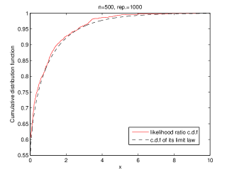
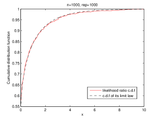
Figure 1. Empirical distribution of the GLR and its limit distribution

Moreover, in the case of more than two components and $k-k_{0}\geq 2$, the limit distribution of the GLR statistic (4.4) under $\mathcal{H}_{0}$ is complicate and not standard (not a $\chi^{2}$ distribution) which poses some difficulty in determining the critical value that will give correct asymptotic size; see Self and Liang (1987). On the other hand, the likelihood ratio statistic

$$W_{n}(\theta):=2log\frac{L(\widehat{\theta})}{L(\theta)}$$ (4.9)

can not be used to construct asymptotic confidence region for the parameter $\theta_{T}$ since its limit law is not the same when $\theta_{T}=0$ and $\theta_{T}>0$.

In figure 1, we illustrate the accuracy of the approximation of distribution of the GLR by its limit $0.5\delta_{0}+0.5\chi_{1}^{2}$; we plot the cumulative distribution function (c.d.f) of both the limit law, and the observed GLR’s obtained from 1000 independent runs of samples with sizes $n=200$, $n=500$ and $n=1000$, with $P_{0}=\mathcal{N}(0,1)$ and $P_{1}=\mathcal{N}(0.5,1)$.

4.2. A simple solution to the problem of testing the number of components in a mixture

We propose the following simple solution : Consider the following set of signed finite measures

$$p_{\theta}:=(1-\theta)p_{0}+\theta p_{1}\text{ where }\theta\in\mathds{R}.$$ (4.10)

This set (of signed finite measures with mass one) obviously contains the mixture model (4.5). In particular, the null value of $\theta_{T}$ (i.e., $\theta_{T}=0$) is an interior point of the parameter space $\mathds{R}$. The likelihood ratio test (for a model of signed measures) cannot be used since the log-likelihood $l(\theta)$ may be infinite (when $\theta<0$ or $\theta>1$). In the context of divergences, this means that the estimate $\widehat{KL_{m}}(P_{0},P_{\theta_{T}})$ may be infinite if we consider the model (4.10), which is due to the fact that the corresponding convex function $\phi(x)=-\log x+x-1$ is infinite on $\mathbb{R}_{-}$. This suggests to use a divergence associated to a convex function $\phi$ which is finite on all $\mathbb{R}$, for instance, the $\chi^{2}$-divergence (which is associated to the convex function $\phi(x)=\frac{1}{2}(x-1)^{2}$). So, in order to perform a test asymptotically of level $\epsilon$ for (4.6), we propose to use the following estimate of the $\chi^{2}$-divergence between $P_{0}$ and $P_{\theta_{T}}$

$$\widetilde{\chi^{2}}(0,\theta_{T})=\sup_{\alpha\in\Theta_{e}}\left\{P_{0}f(0,\alpha)-P_{n}g(0,\alpha)\right\},$$ (4.11)

where $f(0,\alpha)=p_{0}/p_{\alpha}-1$ and $g(0,\alpha)=1/2(p_{0}/p_{\alpha}+1)(p_{0}/p_{\alpha}-1)$ as a consequence of definitions (3.9) and (3.8), and $\Theta_{e}$ is the new parameter space which we define as follows

$$\Theta_{e}:=\left\{\alpha\in\mathds{R}\text{ such that }\int\left|f(0,\alpha)\right|~{}dP_{0}\text{ is finite }\right\}.$$

The value of the parameter $\theta_{T}$ under the null hypothesis $\mathcal{H}_{0}$, i.e., $\theta_{T}=0$, is in the interior of the new parameter space $\Theta_{e}$ which is generally non void. Hence, under conditions of theorem 3.2 where $\Theta$ is replaced by $\Theta_{e}$ and $\theta$ by zero, under $\mathcal{H}_{0}$ the statistic $2n\widetilde{\chi^{2}}(0,\theta_{T})$ converges in distribution to a $\chi^{2}$ random variable with one degree of freedom; the critical region takes then the form

$$CR:=\left\{2n\widetilde{\chi^{2}}(0,\theta_{T})>q_{1,\epsilon}\right\},$$ (4.12)

where $q_{1,\epsilon}$ is the $(1-\epsilon)$-quantile of the $\chi^{2}$ distribution with one degree of freedom. Obviously other divergences which are associated to convex functions finite on all $\mathbb{R}$ can be used. The use of the $\chi^{2}$-divergence is recommended. Indeed, for regular cases (for example for multinomial goodness-of-fit tests) $\chi^{2}$-test is equivalent (in Pitman sense) to the generalized likelihood ratio one; see also Cressie and Read (1984) sections 3.1 and 3.2 for other motivations in favor of the $\chi^{2}$ approach.

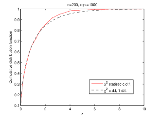
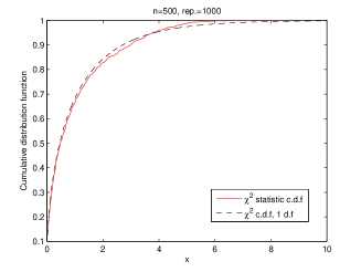
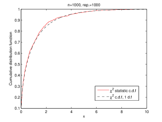
Figure 2. Empirical distribution of the dual $\chi^{2}$-statistic and its limit law

In figure 2, we illustrate the accuracy of the approximation of the distribution of the proposed dual $\chi^{2}$-statistic by the $\chi^{2}(1)$; we plot the cumulative distribution function (c.d.f) of both the limit law, and the dual $\chi^{2}$-statistic obtained from 1000 independent runs of samples with sizes $n=200$, $n=500$ and $n=1000$, with $P_{0}=\mathcal{N}(0,1)$ and $P_{1}=\mathcal{N}(0.5,1)$. We observe that the approximation is as satisfactory as it is in figure 1 for the GLR case, so that the extension of the model to signed finite measures does not affect the quality of the approximation of the limit distribution.

4.3. Confidence regions for the mixture parameters

We propose the following solution to the confidence region problem when the parameter may be a boundary value of the parameter space: The estimate

$$\widetilde{\chi^{2}}(\theta,\theta_{T})=\sup_{\alpha\in\Theta_{e}(\theta)}\left\{P_{\theta}f(\theta,\alpha)-P_{n}g(\theta,\alpha)\right\},$$ (4.13)

where

$$\Theta_{e}(\theta):=\left\{\alpha\in\mathds{R}\text{ such that }\int\left|f(\theta,\alpha)\right|~{}dP_{\theta}\text{ is finite }\right\},$$

can be used to construct asymptotic confidence region for the parameter $\theta_{T}$ with level $(1-\epsilon)$ defined by

$$C:=\left\{\theta\in\Theta\text{ such that }2n\widetilde{\chi^{2}}(\theta,\theta_{T})\leq q_{1,\epsilon}\right\}.$$

In fact, $\lim_{n\rightarrow\infty}P_{\theta_{T}}\left(\theta_{T}\in C\right)=1-\epsilon$ both when $\theta_{T}=0$ or $\theta_{T}>0$ since the statistic $2n\widetilde{\chi^{2}}(\theta_{T},\theta_{T})$ converges in distribution to $\chi^{2}$ random variable with one degree of freedom both when $\theta_{T}=0$ or $\theta_{T}>0$. We give now the form of the critical region and the confidence region in the multivariate case, i.e., in the case of the general model (4.1). For all $\theta\in\Theta$, define the set

$$\Theta_{e}(\theta):=\left\{\alpha\in\mathds{R}^{k}\times A_{1}\times\cdots\times A_{k}\text{ such that }\sum_{i=1}^{k}\alpha_{i}=1\text{ and }\int\left|f(\theta,\alpha)\right|~{}dP_{\theta}\text{ is finite }\right\},$$

and the statistic

$$\widetilde{\chi^{2}}(\Theta_{0},\theta_{T}):=\inf_{\theta\in\Theta_{0}}\widetilde{\chi^{2}}(\theta,\theta_{T}):=\inf_{\theta\in\Theta_{0}}\sup_{\alpha\in\Theta_{e}(\theta)}\left\{P_{\theta}f(\theta,\alpha)-P_{n}g(\theta,\alpha)\right\}.$$

Under some conditions similar to that in theorems 3.1, 3.2 and 3.3, we can prove, under the null hypothesis $\mathcal{H}_{0}$ in (4.3), that the statistic $2n\widetilde{\chi^{2}}(\Theta_{0},\theta_{T})$ converges in distribution to $\chi^{2}$ random variable with $(k-k_{0})$ degrees of freedom. Also, the statistic $2n\widetilde{\chi^{2}}(\theta,\theta_{T})$ when $\theta=\theta_{T}$ converges in distribution to $\chi^{2}$ random variable with $d:=k-1+d_{1}+\cdots+d_{k}$ degrees of freedom in both case when $\theta_{T}$ is a boundary value or not. Hence, the critical region is given by

$$CR:=\left\{2n\widetilde{\chi^{2}}(\Theta_{0},\theta_{T})>q_{k-k_{0},\epsilon}\right\},$$

and

$$C:=\left\{\theta\in\Theta\text{ such that }2n\widetilde{\chi^{2}}(\theta,\theta_{T})\leq q_{d,\epsilon}\right\}$$

is an asymptotic confidence region for $\theta_{T}$ of level $\epsilon$ both when $\theta_{T}$ is a boundary value or not.

4.4. Approximation of the power function of the likelihood ratio statistic: simulation results

In the context of the exponential model $p_{\theta}(x)=\theta\exp\left\{\theta x\right\}$, we consider the problem of testing

$$\mathcal{H}_{0}:\theta_{T}=1\quad\text{versus}\quad\mathcal{H}_{1}:\theta_{T}\neq 1$$

using the GLR. We recall that the power function of the GLR test is

$$\theta_{T}\mapsto\beta(\theta_{T}):=P_{\theta_{T}}\left\{2n\widehat{KL_{m}}\left(1,\theta_{T}\right)\geq q_{1,0.5}\right\}$$ (4.14)

and its approximation is

$$\widehat{\beta}(\theta_{T})=1-F_{\mathcal{N}}\left(\frac{\sqrt{n}}{\sigma_{\phi}(1,\theta_{T})}\left[\frac{1}{2n}q_{1,0.05}-KL_{m}(1,\theta_{T})\right]\right)$$ (4.15)

where $F_{\mathcal{N}}$ is the cumulative distribution function of a normal random variable with mean zero and variance one, and $\phi(x)=-\log x+x-1$; see remarks 3.3 and 3.4 above. The power function (4.14) is plotted (with continuous line) for sample sizes $n=50$, $n=100$, $n=300$ and $n=500$, and for different values of $\theta_{T}$. Each power entry was obtained from $1000$ independent runs. The approximation (4.15) is plotted as a function of $\theta_{T}$ by a dashed line. We observe (see figure 3) that the approximation is accurate for alternatives which are not “close to” the null hypothesis even for moderate sample sizes.

Figure 3. Approximation of the power function

5. Concluding remarks and possible developments

We have addressed the parametric estimation and test problems. We have introduced new estimation and test procedure using divergence minimization and duality technique for discrete or continuous parametric models, avoiding the smoothing method. The procedure leads to optimal estimates for the parameter model and for the divergences. It includes both the discrete (finite or infinite) and the continuous support cases. It extends the maximum likelihood method for both estimation and test problems. Moreover, the procedure and the divergences framework permit to obtain the limit laws of the proposed estimates and the test statistics both under the null and the alternative (simple or composite) hypotheses, including the generalized likelihood ratio statistic. As a by-product, we obtain explicit power functions in a general case for simple or composite parametric test problems, and approximations of the minimal sample size which guarantees a desired power for a given alternative. A new test and new asymptotic confidence regions are proposed in the case where the parameter may be a boundary value of the parameter space. Many problems remain to be studied in the future, such as the choice of the divergence which leads to an “optimal” (in some sense) estimate or test in terms of efficiency and robustness, construction of convergent estimates and test statistics by divergence when the maximum likelihood is not consistent (for example for location family for which the expectation does not exists), the Bartlett correctability and the large deviation properties of the proposed statistics $\widehat{D_{\phi}}.$

6. Appendix

Proof of proposition 3.1

(1) We will prove the consistency of the estimate $\widehat{D_{\phi}}(\theta,\theta_{T})$. We have

$$\left|\widehat{D_{\phi}}(\theta,\theta_{T})-D_{\phi}(\theta,\theta_{T})\right|=\left|P_{n}h(\theta,\widehat{\alpha}_{\phi}(\theta))-P_{\theta_{T}}h(\theta,\theta_{T})\right|:=|A|,$$

which implies

$$P_{n}h(\theta,\theta_{T})-P_{\theta_{T}}h(\theta,\theta_{T})\leq A\leq P_{n}h(\theta,\widehat{\alpha}_{\phi}(\theta))-P_{\theta_{T}}h(\theta,\widehat{\alpha}_{\phi}(\theta)).$$

Both the RHS and the LHS terms in the above display go to $0$, under condition (c.2). This implies that $A$ tends to $0$.
(2) For the consistency of $\widehat{\alpha}_{\phi}(\theta)$, we refer to van der Vaart (1998) theorem 5.7.

Proof of theorem 3.2

(a) Using (A.1), simple calculus give

$$P_{\theta_{T}}(\partial/\partial\alpha)h(\theta,\alpha)=0$$ (6.1)

and

$$P_{\theta_{T}}(\partial^{2}/\partial\alpha^{2})h(\theta,\theta_{T})=-\int\phi^{\prime\prime}(p_{\theta}/p_{\theta_{T}})(p_{\theta}^{2}/p_{\theta_{T}}^{3})p_{\theta_{T}}^{\prime}p_{\theta_{T}}^{\prime}{}^{T}~{}d\lambda=:-S.$$ (6.2)

Observe that the matrix $S$ is symmetric and positive since the second derivative $\phi^{\prime\prime}$ is nonnegative by the convexity of $\phi$. Let $U_{n}(\theta_{T}):=P_{n}(\partial/\partial\alpha)h(\theta,\theta_{T})$, and use (6.1) and (A.2) in connection with the Central Limit Theorem (CLT) to see that

$$\sqrt{n}U_{n}(\theta_{T})\rightarrow\mathcal{N}(0,M).$$ (6.3)

Also, let $V_{n}(\theta_{T}):=P_{n}(\partial^{2}/\partial\alpha^{2})h(\theta,\theta_{T})$, and use (6.2) and (A.2) in connection with the Law of Large Numbers (LLN) to conclude that

$$V_{n}(\theta_{T})\rightarrow-S~{}~{}(a.s).$$ (6.4)

Using the fact that $P_{n}(\partial/\partial\alpha)h(\theta,\widehat{\alpha})=0$ and a Taylor expansion of $P_{n}(\partial/\partial\alpha)h(\theta,\widehat{\alpha})$ in $\widehat{\alpha}$ around $\theta_{T}$, we obtain

$$0=P_{n}(\partial/\partial\alpha)h(\theta,\widehat{\alpha})=P_{n}(\partial/\partial\alpha)h(\theta,\theta_{T})+(\widehat{\alpha}-\theta_{T})^{T}P_{n}(\partial^{2}/\partial\alpha^{2})h(\theta,\theta_{T})+o_{p}(n^{-1/2}).$$

Hence,

$$\sqrt{n}\left(\widehat{\alpha}-\theta_{T}\right)=-V_{n}(\theta_{T})^{-1}\sqrt{n}U_{n}(\theta_{T})+o_{p}(1).$$ (6.5)

Using (6.3) and (6.4) and Slutsky theorem, we conclude then

$$\sqrt{n}\left(\widehat{\alpha}-\theta_{T}\right)\to\mathcal{N}\left(0,V_{\phi}(\theta,\theta_{T})\right)$$ (6.6)

where $V_{\phi}(\theta,\theta_{T})$ is given in part (a) of theorem 3.2. When $\theta_{T}=\theta$, direct calculus shows that $V_{\phi}(\theta,\theta_{T})=I_{\theta_{T}}^{-1}$.

(b) Assume that $\theta_{T}=\theta$. From (6.5), using the convergence (6.4), we get

$$\sqrt{n}\left(\widehat{\alpha}-\theta_{T}\right)=S^{-1}\sqrt{n}U_{n}(\theta_{T})+o_{p}(1).$$ (6.7)

On the other hand, a Taylor expansion of $\left[2n/\phi^{\prime\prime}(1)\right]\widehat{D_{\phi}}(\theta,\theta_{T})=\left[2n/\phi^{\prime\prime}(1)\right]P_{n}(\partial/\partial\alpha)h(\theta,\widehat{\alpha})$ in $\widehat{\alpha}$ around $\theta_{T}$, using the fact that $P_{n}h(\theta,\theta_{T})=0$ when $\theta_{T}=\theta$, gives

$$\frac{2n}{\phi^{\prime\prime}(1)}\widehat{D_{\phi}}(\theta,\theta_{T})=\frac{2n}{\phi^{\prime\prime}(1)}U_{n}^{T}(\widehat{\alpha}-\theta_{T})+\frac{2n}{\phi^{\prime\prime}(1)}(\widehat{\alpha}-\theta_{T})^{T}V_{n}(\widehat{\alpha}-\theta_{T})+o_{p}(1).$$

Use (6.4), (6.7) and the fact that $S=-\phi^{\prime\prime}(1)I_{\theta_{T}}$ when $\theta_{T}=\theta$ to conclude that

$$\frac{2n}{\phi^{\prime\prime}(1)}\widehat{D_{\phi}}(\theta,\theta_{T})={\phi^{\prime\prime}(1)}^{-2}\sqrt{n}U_{n}^{T}I_{\theta_{T}}^{-1}\sqrt{n}U_{n}+o_{p}(1).$$

Finally, use the convergence (6.3) and the fact that $M=\phi^{\prime\prime}(1)^{2}I_{\theta_{T}}$ when $\theta=\theta_{T}$, to conclude that $\left[2n/\phi^{\prime\prime}(1)\right]\widehat{D_{\phi}}(\theta,\theta_{T})$ converges in distribution to a $\chi^{2}$ variable with $d$ degrees of freedom when $\theta=\theta_{T}$.

(c) Assume that $\theta_{T}\neq\theta$. A Taylor expansion of $\widehat{D_{\phi}}(\theta,\theta_{T})=P_{n}h(\theta,\widehat{\alpha})$, in $\widehat{\alpha}$ around $\theta_{T}$, using the fact that $P_{\theta_{T}}(\partial/\partial\alpha)h(\theta,\theta_{T})=0$, gives $\widehat{D_{\phi}}(\theta,\theta_{T})=P_{n}h(\theta,\theta_{T})+o_{p}(n^{-1/2})$. Hence,

$$\sqrt{n}\left(\widehat{D_{\phi}}(\theta,\theta_{T})-D_{\phi}(\theta,\theta_{T})\right)=\sqrt{n}\left[P_{n}h(\theta,\theta_{T})-P_{\theta_{T}}h(\theta,\theta_{T})\right]+o_{p}(1),$$

which under assumption (A.3), by the CLT, converges in distribution to a centred normal variable with variance $\sigma_{\phi}^{2}(\theta,\theta_{T})=P_{\theta_{T}}h(\theta,\theta_{T})^{2}-\left(P_{\theta_{T}}h(\theta,\theta_{T})\right)^{2}$.

Proof of theorem 3.3

(a) For any $\alpha=\theta_{T}+un^{-1/3}$ with $|u|\leq 1$, consider a Taylor expansion of $P_{n}h(\theta,\alpha)$ in $\alpha$ around $\theta_{T}$, and use (A.1) to see that

$$nP_{n}h(\theta,\alpha)-nP_{n}h(\theta,\theta_{T})=n^{2/3}u^{T}U_{n}+2^{-1}n^{1/3}u^{T}V_{n}u+O(1)~{}(a.s.)$$

uniformly on $u$ with $|u|\leq 1$. Now, use (6.4) and the fact that $U_{n}=O\left(n^{-1/2}(\log\log n)^{1/2}\right)$ (a.s) to conclude that

$$nP_{n}h(\theta,\alpha)-nP_{n}h(\theta,\theta_{T})=O\left(n^{1/6}(\log\log n)^{1/2}\right)-2^{-1}u^{T}Sun^{1/3}+O(1)~{}(a.s.)$$

uniformly on $u$ with $|u|\leq 1$. Hence, uniformly on the surface of the ball $B$ (i.e., uniformly on $u$ with $|u|=1$), we have

$$nP_{n}h(\theta,\alpha)-nP_{n}h(\theta,\theta_{T})\leq O\left(n^{1/6}(\log\log n)^{1/2}\right)-2^{-1}cn^{1/3}+O(1)~{}~{}(a.s.)$$ (6.8)

where $c$ is the smallest eigenvalue of the matrix $S$. Note that $c$ is positive since $S$ is positive definite (it is symmetric, positive and non singular by assumption A.2). In view of $(\ref{eqn5})$, by the continuity of $\alpha\mapsto P_{n}h(\theta,\alpha)-nP_{n}h(\theta,\theta_{T})$ and since it takes value zero on $\alpha=\theta_{T}$ and is asymptotically negative on the surface of $B$, it holds that as $n\rightarrow\infty$, with probability one, $\alpha\mapsto P_{n}h(\theta,\alpha)$ attains its maximum value at some point $\widetilde{\alpha}_{\phi}(\theta)$ in the interior of the ball $B$, and therefore the estimate $\widetilde{\alpha}_{\phi}(\theta)$ satisfies $P_{n}(\partial/\partial\alpha)h(\theta,\widetilde{\alpha})=0$ and $\widetilde{\alpha}-\theta_{T}=O(n^{-1/3})$.

The proofs of parts (b), (c) and (d) are similar to those of parts (a), (b) and (d) in theorem 3.2. Hence, they are omitted.

Proof of proposition 3.4

We prove (1). For all $\theta\in\Theta$, under condition (c.4-5-6), we prove that $\sup_{\theta\in\Theta}\|\widehat{\alpha}_{\phi}(\theta)-\theta_{T}\|$ tends to $0$. By the very definition of $\widehat{\alpha}_{\phi}(\theta)$ and the condition (c.5), we have

$$P_{n}h(\theta,\widehat{\alpha}_{\phi}(\theta)) \geq P_{n}h(\theta,\theta_{T})$$

$$\geq P_{\theta_{T}}h(\theta,\theta_{T})-o_{p}(1),$$

where $o_{p}(1)$ does not depend upon $\theta$ (due to condition (c.5)). Hence, we have for all $\theta\in\Theta$

$$P_{\theta_{T}}h(\theta,\theta_{T})-P_{\theta_{T}}h(\theta,\widehat{\alpha}_{\phi}(\theta))\leq P_{n}h(\theta,\widehat{\alpha}_{\phi}(\theta))-P_{\theta_{T}}h(\theta,\widehat{\alpha}_{\phi}(\theta))+o_{p}(1).$$ (6.9)

The RHS term is less than $\sup_{\left\{\theta,\alpha\in\Theta\right\}}\left|P_{n}h(\theta,\alpha)-P_{\theta_{T}}h(\theta,\alpha)\right|$ $+o_{p}(1)$ which, by (c.5), tends to $0$. Let $\epsilon>0$ be such that $\sup_{\theta\in\Theta}\|\widehat{\alpha}_{\phi}(\theta)-\theta_{T}\|>\epsilon$. There exists some $a_{n}\in\Theta$ such that $\|\widehat{\alpha}_{\phi}(a_{n})-\theta_{T}\|>\epsilon$. Together with $(c.5.a)$, there exists some $\eta>0$ such that $P_{\theta_{T}}h(a_{n},\theta_{T})-P_{\theta_{T}}h(a_{n},\widehat{\alpha}_{\phi}(a_{n}))>\eta$. We then conclude that

$$P\left\{\sup_{\theta\in\Theta}\|\widehat{\alpha}_{\phi}(\theta)-\theta_{T}\|>\epsilon\right\}\leq P\left\{P_{\theta_{T}}h(a_{n},\theta_{T})-P_{\theta_{T}}h(a_{n},\widehat{\alpha}_{\phi}(\theta))>\eta\right\},$$

and the RHS term tends to $0$ by (6.9). This concludes the proof of part (1).
We prove (2). By the very definition of $\widehat{\theta}_{\phi}$, conditions (c.5) and (c.6) and part (1), we have

$$P_{n}h(\widehat{\theta}_{\phi},\widehat{\alpha}_{\phi}(\widehat{\theta}_{\phi})) \leq P_{n}h(\theta_{T},\widehat{\alpha}_{\phi}(\theta_{T}))$$

$$\leq P_{\theta_{T}}h(\theta_{T},\widehat{\alpha}_{\phi}(\widehat{\theta}_{\phi}))-o_{p}(1),$$

from which

$$P_{\theta_{T}}h(\widehat{\theta}_{\phi},\widehat{\alpha}_{\phi}(\widehat{\theta}_{\phi}))-P_{\theta_{T}}h(\theta_{T},\widehat{\alpha}_{\phi}(\widehat{\theta}_{\phi})) \leq P_{\theta_{T}}h(\widehat{\theta}_{\phi},\widehat{\alpha}_{\phi}(\widehat{\theta}_{\phi}))-P_{n}h(\widehat{\theta}_{\phi},\widehat{\alpha}_{\phi}(\widehat{\theta}_{\phi}))+o_{p}(1)$$ (6.10)

$$\leq \sup_{\left\{\theta,\alpha\in\Theta\right\}}\left|P_{n}h(\theta,\alpha)-P_{\theta_{T}}h(\theta,\alpha)\right|+o_{p}(1).$$

Further, by part (1) and condition (c.5.b), for any positive $\epsilon$, there exists $\eta>0$ such that

$$P\left\{\|\widehat{\theta}_{\phi}-\theta_{T}\|>\epsilon\right\}\leq P\left\{P_{\theta_{T}}h(\widehat{\theta}_{\phi},\widehat{\alpha}_{\phi}(\widehat{\theta}_{\phi}))-P_{\theta_{T}}h(\theta_{T},\widehat{\alpha}_{\phi}(\widehat{\theta}_{\phi}))>\eta\right\},$$

and the RHS term, under condition (c.5), tends to $0$ by (6.10). This concludes the proof.

Proof of theorem 3.5

Under condition (A.5), simple calculus give

$$P_{\theta_{T}}\frac{\partial}{\partial\alpha}h(\theta_{T},\theta_{T})=P_{\theta_{T}}\frac{\partial}{\partial\theta}h(\theta_{T},\theta_{T})=P_{\theta_{T}}\frac{\partial^{2}}{\partial\alpha\partial\theta}h(\theta_{T},\theta_{T})=P_{\theta_{T}}\frac{\partial^{2}}{\partial\theta\partial\alpha}h(\theta_{T},\theta_{T})=0,$$ (6.11)

$$-P_{\theta_{T}}\frac{\partial^{2}}{\partial\alpha^{2}}h(\theta_{T},\theta_{T})=P_{\theta_{T}}\frac{\partial^{2}}{\partial\theta^{2}}h(\theta_{T},\theta_{T})=\phi^{\prime\prime}(1)I_{\theta_{T}},$$ (6.12)

and

$$P_{\theta_{T}}\left[\frac{\partial}{\partial\theta}h(\theta_{T},\theta_{T})\right]\left[\frac{\partial}{\partial\theta}h(\theta_{T},\theta_{T})\right]^{T} = P_{\theta_{T}}\left[\frac{\partial}{\partial\alpha}h(\theta_{T},\theta_{T})\right]\left[\frac{\partial}{\partial\alpha}h(\theta_{T},\theta_{T})\right]^{T}$$ (6.13)

$$= -P_{\theta_{T}}\left[\frac{\partial}{\partial\alpha}h(\theta_{T},\theta_{T})\right]\left[\frac{\partial}{\partial\theta}h(\theta_{T},\theta_{T})\right]^{T}$$

$$= {\phi^{\prime\prime}(1)}^{2}I_{\theta_{T}}.$$

Denote $U_{n}(\theta,\theta_{T}):=P_{n}(\partial/\partial\alpha)h(\theta,\theta_{T})$, $V_{n}(\theta,\theta_{T}):=P_{n}(\partial^{2}/\partial\alpha^{2})h(\theta,\theta_{T})$, $S(\theta,\theta_{T}):=-P_{\theta_{T}}(\partial^{2}/\partial\alpha^{2})h(\theta,\theta_{T})$ and $a_{n}^{T}:=\left((\widehat{\theta}_{\phi}-\theta_{T})^{T},(\widehat{\alpha}_{\phi}(\widehat{\theta}_{\phi})-\theta_{T})^{T}\right)^{T}$. Under conditions (A.4-5), by a Taylor expansion, we obtain

$$\sqrt{n}a_{n}=\sqrt{n}\left[\begin{array}[]{cc}\frac{1}{\phi^{\prime\prime}(1)}I_{\theta_{T}}^{-1}&0\\ 0&\frac{-1}{\phi^{\prime\prime}(1)}I_{\theta_{T}}^{-1}\end{array}\right]\left[\begin{array}[]{c}-P_{n}\frac{\partial}{\partial\theta}h(\theta_{T},\theta_{T})\\ -P_{n}\frac{\partial}{\partial\alpha}h(\theta_{T},\theta_{T})\end{array}\right]+o_{p}(1).$$

We therefore deduce, by the CLT, that, under condition (A.6), $\sqrt{n}a_{n}$ converges in distribution to a centred normal variable with covariance matrix

$$\mathbb{V}=\left[\begin{array}[]{cc}I_{\theta_{T}}^{-1}&I_{\theta_{T}}^{-1}\\ I_{\theta_{T}}^{-1}&I_{\theta_{T}}^{-1}\end{array}\right],$$

which completes the proof of theorem 3.5.

Proof of theorem 3.6

(a) Using condition (A.5) and (6.11), we can write

$$U_{n}(\theta,\theta_{T}):=U_{n}(\theta_{T},\theta_{T})+o(n^{-1/3})~{}(a.s.)$$ (6.14)

and

$$V_{n}(\theta,\theta_{T}):=V_{n}(\theta_{T},\theta_{T})+O(n^{-1/3})~{}(a.s.),$$ (6.15)

uniformly on $\theta\in B(\theta_{T},n^{-1/3})$. On the other hand, for any $\alpha=\theta_{T}+un^{-1/3}$ with $|u|\leq 1$, by a Taylor expansion using condition (A.5), we obtain

$$nP_{n}h(\theta,\alpha)-nP_{n}h(\theta,\theta_{T})=n^{2/3}u^{T}U_{n}(\theta,\theta_{T})+2^{-1}n^{1/3}u^{T}V_{n}(\theta,\theta_{T})u+O(1)~{}(a.s.)$$

uniformly on $\theta\in B(\theta_{T},n^{-1/3})$ and $u$ with $|u|\leq 1$. Combining this with (6.14) and (6.15) to see that

$$nP_{n}h(\theta,\alpha)-nP_{n}h(\theta,\theta_{T})=n^{2/3}u^{T}U_{n}(\theta_{T},\theta_{T})+2^{-1}n^{1/3}u^{T}V_{n}(\theta_{T},\theta_{T})u+o(n^{1/3})~{}(a.s.)$$

uniformly on $\theta\in B(\theta_{T},n^{-1/3})$ and $u$ with $|u|\leq 1$. Now, from this, using the fact that $U_{n}(\theta_{T},\theta_{T})=O\left(n^{-1/2}(\log\log n)^{1/2}\right)$ (a.s.) and $V_{n}(\theta_{T},\theta_{T})=-S(\theta_{T},\theta_{T})+o(1)$ (a.s.), we obtain

$$nP_{n}h(\theta,\alpha)-nP_{n}h(\theta,\theta_{T})=O\left(n^{1/6}(\log\log n)^{1/2}\right)-2^{-1}n^{1/3}u^{T}S(\theta_{T},\theta_{T})u+o(n^{1/3})~{}(a.s.)$$ (6.16)

uniformly on $\theta\in B(\theta_{T},n^{-1/3})$ and $u$ with $|u|\leq 1$. Hence, uniformly on $\alpha$ in the surface of the ball $B(\theta_{T},n^{-1/3})$ (i.e., uniformly on $u$ with $|u|=1$), we have

$$nP_{n}h(\theta,\alpha)-nP_{n}h(\theta,\theta_{T})\leq O\left(n^{1/6}(\log\log n)^{1/2}\right)-2^{-1}\phi^{\prime\prime}(1)cn^{1/3}+o(n^{1/3})~{}(a.s.)$$ (6.17)

(uniformly on $\theta\in B(\theta_{T},n^{-1/3}))$ where $c>0$ is the smallest eigenvalue of the matrix $I_{\theta_{T}}=\phi^{\prime\prime}(1)^{-1}S(\theta_{T},\theta_{T})$. Hence, by the continuity of the function $\alpha\mapsto nP_{n}h(\theta,\alpha)-nP_{n}h(\theta,\theta_{T})$ and since it takes value zero when $\alpha=\theta_{T}$ and is asymptotically negative with respect to $\alpha$ on the surface of $B$, it holds that, as $n$ tends to $\infty$, with probability one, the function $\alpha\mapsto P_{n}h(\theta,\alpha)$ attains it maximum value at some point $\widetilde{\alpha}_{\phi}(\theta)$ in the interior of $B(\theta_{T},n^{-1/3})$, and this holds for all $\theta\in B(\theta_{T},n^{-1/3})$. Further, since (6.16) holds uniformly on $\theta\in B(\theta_{T},n^{-1/3})$, we conclude that

$$\widetilde{\alpha}_{\phi}(\theta)-\theta_{T}=O(n^{-1/3})~{}(a.s.)\text{ uniformly on }\theta\in B(\theta_{T},n^{-1/3}).$$ (6.18)

We now prove that, as $n\rightarrow\infty$, with probability one, the function $\theta\mapsto P_{n}(\theta,\widehat{\alpha}_{\phi}(\theta))$ attains its minimum value at some point $\widetilde{\theta}_{\phi}$ in the interior of the ball $B(\theta_{T},n^{-1/3})$. Here, $\widetilde{\alpha}_{\phi}(\theta)$ is any value in the interior of $B(\theta_{T},n^{-1/3})$ which maximizes $\alpha\mapsto P_{n}h(\theta,\alpha)$. It exists by the above arguments. For any $\theta=\theta_{T}+vn^{-1/3}$ with $|v|\leq 1$, by a Taylor expansion of $nP_{n}h(\theta,\widetilde{\alpha}_{\phi}(\theta))$ in $\theta$ and $\widetilde{\alpha}_{\phi}(\theta)$ around $\theta_{T}$ , and a Taylor expansion of $nP_{n}h(\theta_{T},\widetilde{\alpha}_{\phi}(\theta_{T}))$ in $\widetilde{\alpha}_{\phi}(\theta_{T})$ around $\theta_{T}$, using (6.18) and (6.11), we obtain

$$nP_{n}h(\theta,\widetilde{\alpha}_{\phi}(\theta))-nP_{n}h(\theta_{T},\widetilde{\alpha}_{\phi}(\theta_{T})) = n^{2/3}v^{T}P_{n}(\partial/\partial\theta)h(\theta_{T},\theta_{T})+$$

$$2^{-1}n^{1/3}v^{T}\left[P_{n}(\partial^{2}/\partial\theta^{2})h(\theta_{T},\theta_{T})\right]v+o(n^{1/3})~{}(a.s.)$$

uniformly on $v$ with $|v|\leq 1$. Hence, from this, using the fact that
$P_{n}(\partial/\partial\theta)h(\theta_{T},\theta_{T})=O\left(n^{-1/2}(\log\log n)^{1/2}\right)$ (a.s.) and $P_{n}(\partial^{2}/\partial\theta^{2})h(\theta_{T},\theta_{T})=\phi^{\prime\prime}(1)I_{\theta_{T}}+o(1)$ (a.s.), we conclude that

$$nP_{n}h(\theta,\widetilde{\alpha}_{\phi}(\theta))-nP_{n}h(\theta_{T},\widetilde{\alpha}_{\phi}(\theta_{T}))=O\left(n^{1/6}(\log\log n)^{1/2}\right)+2^{-1}\phi^{\prime\prime}(1)v^{T}I_{\theta_{T}}vn^{1/3}+o(n^{1/3})~{}(a.s.)$$

uniformly on $v$ with $|v|\leq 1$. Hence, uniformly on $\theta$ in the surface of the ball $B(\theta_{T},n^{-1/3})$ (i.e., uniformly on $v$ with $|v|=1$), we obtain

$$nP_{n}h(\theta,\widetilde{\alpha}_{\phi}(\theta))-nP_{n}h(\theta_{T},\widetilde{\alpha}_{\phi}(\theta_{T}))\geq O\left(n^{1/6}(\log\log n)^{1/2}\right)+2^{-1}\phi^{\prime\prime}(1)cn^{1/3}+o(n^{1/3})~{}(a.s.)$$

where $c>0$ is the smallest eigenvalue of $I_{\theta_{T}}$. This implies that

$$n^{2/3}P_{n}h(\theta,\widetilde{\alpha}_{\phi}(\theta))-n^{2/3}P_{n}h(\theta_{T},\widetilde{\alpha}_{\phi}(\theta_{T}))\geq O\left(n^{-1/6}(\log\log n)^{1/2}\right)+2^{-1}\phi^{\prime\prime}(1)c+o(1)~{}(a.s.)$$

uniformly on $\theta$ in the surface of the ball $B(\theta_{T},n^{-1/3})$. The left hand side of the above display equals zero when $\theta=\theta_{T}$ and is positive when $\theta$ is in the surface of the ball $B(\theta_{T},n^{-1/3})$ (for $n$ sufficiently large). This implies that, as $n\rightarrow\infty$, with probability one, the function $\theta\mapsto P_{n}h(\theta,\widetilde{\alpha}_{\phi}(\theta))$ attains its minimum value at some point $\widetilde{\theta}_{\phi}$ in the interior of the ball $B$. This concludes the proof of part (a).

(b) See the proof of theorem 3.5.

Proof of theorem 3.7

We have

$$\widehat{D_{\phi}}(\Theta_{0},\theta_{T}) := \inf_{\beta\in B_{0}}\sup_{\alpha\in\Theta}P_{n}h\left(s(\beta),\alpha\right).$$

$$= P_{n}h\left(s(\widehat{\beta}),\widehat{\alpha}\right),$$

in which as in the proof of theorem 3.5, $s(\widehat{\beta})$ and $\widehat{\alpha}$ are solutions of the system of equations

$$\left\{\begin{array}[]{ccc}P_{n}\frac{\partial}{\partial\beta}h\left(s(\widehat{\beta}),\widehat{\alpha}\right)&=&0\\ P_{n}\frac{\partial}{\partial\alpha}h\left(s(\widehat{\beta}),\widehat{\alpha}\right)&=&0.\end{array}\right.$$

In the first equation the partial derivative is intended w.r.t. the first variable $\beta$ in $s(\beta)$ and in the second one w.r.t. the second variable $\alpha$. A Taylor expansion of $P_{n}\frac{\partial}{\partial\beta}h\left(s(\widehat{\beta}),\widehat{\alpha}\right)$ and $P_{n}\frac{\partial}{\partial\alpha}h\left(s(\widehat{\beta}),\widehat{\alpha}\right)$ in a neighborhood of $(\beta_{T},\theta_{T})$ gives

$$\left[\begin{array}[]{c}-P_{n}\frac{\partial}{\partial\beta}h(s(\beta_{T}),\theta_{T})\\ -P_{n}\frac{\partial}{\partial\alpha}h(s(\beta_{T}),\theta_{T})\end{array}\right]=\left[\begin{array}[]{cc}P_{\theta_{T}}\frac{\partial^{2}}{\partial\beta^{2}}h(s(\beta_{T}),\theta_{T})&P_{\theta_{T}}\frac{\partial^{2}}{\partial\beta\partial\alpha}h(s(\beta_{T}),\theta_{T})\\ P_{\theta_{T}}\frac{\partial^{2}}{\partial\alpha\partial\beta}h(s(\beta_{T}),\theta_{T})&P_{\theta_{T}}\frac{\partial^{2}}{\partial\beta^{2}}h(s(\beta_{T}),\theta_{T})\end{array}\right]b_{n}+o_{p}(1),$$ (6.19)

where $b_{n}:=\left((\widehat{\beta}-\beta_{T})^{T},(\widehat{\alpha}-\theta_{T})^{T}\right)^{T}$. This implies that $b_{n}=O_{p}(n^{-1/2})$. So, by a Taylor expansion of $\widehat{D_{\phi}}(\Theta_{0},\theta_{T})$ around $(\beta_{T},\theta_{T})$, we obtain

$$\frac{2n}{\phi^{\prime\prime}(1)}T_{n}^{\phi}=U_{n}^{T}A^{-1}U_{n}-V_{n}^{T}B^{-1}V_{n}+o_{p}(1),$$ (6.20)

where

$$U_{n}:=\frac{\sqrt{n}}{\phi^{\prime\prime}(1)}P_{n}\frac{\partial}{\partial\alpha}h\left(s(\beta_{T}),\theta_{T}\right),\quad V_{n}:=\frac{\sqrt{n}}{\phi^{\prime\prime}(1)}P_{n}\frac{\partial}{\partial\beta}h(s(\beta_{T}),\theta_{T}),$$

$$A:=-\frac{1}{\phi^{\prime\prime}(1)}P_{\theta_{T}}\frac{\partial^{2}}{\partial\alpha^{2}}h(s(\beta_{T}),\theta_{T}),\quad B:=\frac{1}{\phi^{\prime\prime}(1)}P_{\theta_{T}}\frac{\partial^{2}}{\partial\beta^{2}}h(s(\beta_{T}),\theta_{T}).$$

By (6.12), it holds $A=I_{\theta_{T}}$. On the other hand,

$$\frac{\partial}{\partial\beta}h\left(s(\beta_{T}),\theta_{T}\right) = {\left[\frac{\partial}{\partial\beta}s(\beta_{T})\right]}^{T}\frac{\partial}{\partial s(\beta)}h\left(s(\beta_{T}),\theta_{T}\right)$$

$$= {\left[S(\beta_{T})\right]}^{T}\frac{\partial}{\partial s(\beta)}h\left(s(\beta_{T}),\theta_{T}\right).$$

Moreover, using the fact that $\phi^{\prime}(1)=0$, we can see that $\frac{\partial}{\partial s(\beta)}h\left(s(\beta_{T}),\theta_{T}\right)=-\frac{\partial}{\partial\alpha}h\left(s(\beta_{T}),\theta_{T}\right)$, which implies

$$P_{\theta_{T}}\frac{\partial}{\partial\beta}h\left(s(\beta_{T}),\theta_{T}\right)={\left[S(\beta_{T})\right]}^{T}\left[-P_{\theta_{T}}\frac{\partial}{\partial\alpha}h\left(s(\beta_{T}),\theta_{T}\right)\right].$$

In the same way, we obtain

$$P_{\theta_{T}}\frac{\partial^{2}}{\partial\beta^{2}}h\left(s(\beta_{T}),\theta_{T}\right)={\left[S(\beta_{T})\right]}^{T}\left[-P_{\theta_{T}}\frac{\partial^{2}}{\partial\alpha^{2}}h\left(s(\beta_{T}),\theta_{T}\right)\right]\left[S(\beta_{T})\right].$$

It follows that $V_{n}={\left[S(\beta_{T})\right]}^{T}U_{n}$ and $B={\left[S(\beta_{T})\right]}^{T}I_{\theta_{T}}S(\beta_{T})$. Combining this result with (6.20), we get

$$\frac{2n}{\phi^{\prime\prime}(1)}\widehat{D_{\phi}}(\Theta_{0},\theta_{T})=U_{n}^{T}\left[I_{\theta_{T}}^{-1}-S(\beta_{T})B^{-1}{S(\beta_{T})}^{T}\right]U_{n}+o_{p}(1),$$

which is precisely the asymptotic expression for the Wilks likelihood ratio statistic for composite hypotheses. The proof is completed following therefore the same arguments as for the Wilks likelihood ratio statistic; see e.g. Sen and Singer (1993) chapter 5.

Proof of theorem 3.8

The proofs of part (a) and (b) are similar to the proofs of part (a) and (b) of theorem 3.7, hence they are omitted.

(c) Using (3.4) and (3.14 ), we can see that $D_{\phi}(\Theta_{0},\theta_{T})$ can be written as

$$D_{\phi}(\Theta_{0},\theta_{T}) := \inf_{\beta\in B_{0}}D_{\phi}(s(\beta),\theta_{T})=D_{\phi}(s(\beta^{*}),\theta_{T})$$ (6.21)

$$= \sup_{\alpha\in\Theta}P_{\theta_{T}}h(s(\beta^{*}),\alpha)=P_{\theta_{T}}h(s(\beta^{*}),\theta_{T}).$$

On the other hand, by a Taylor expansion of $\widehat{D_{\phi}}(\Theta_{0},\theta_{T})=P_{n}h(s(\widehat{\beta}),\widehat{\alpha}_{\phi}(\widehat{\beta}))$ in $\widehat{\beta}$ and $\widehat{\alpha}_{\phi}(\widehat{\beta})$ around $\beta^{*}$ and $\theta_{T}$, we obtain

$$\widehat{D_{\phi}}(\Theta_{0},\theta_{T})=P_{n}h(s(\beta^{*}),\theta_{T})+o_{p}(n^{-1/2}).$$

Combining this with (6.21) to conclude that

$$\sqrt{n}\left[\widehat{D_{\phi}}(\Theta_{0},\theta_{T})-D_{\phi}(\Theta_{0},\theta_{T})\right]=\sqrt{n}\left[P_{n}h(s(\beta^{*}),\theta_{T})-P_{\theta_{T}}h(s(\beta^{*}),\theta_{T})\right]+o_{p}(1)$$

which, by the CLT, converges to a centred normal variable with variance

$$\sigma_{\phi}^{2}(\beta^{*},\theta_{T})=P_{\theta_{T}}h(s(\beta^{*}),\theta_{T})^{2}-\left(P_{\theta_{T}}h(s(\beta^{*}),\theta_{T})\right)^{2}.$$

This ends the proof.

References

- Basu and Lindsay (1994) Basu, A. and Lindsay, B. G. (1994). Minimum disparity estimation for continuous models: efficiency, distributions and robustness. Ann. Inst. Statist. Math., 46(4), 683–705.
- Beran (1977) Beran, R. (1977). Minimum Hellinger distance estimates for parametric models. Ann. Statist., 5(3), 445–463.
- Berlinet (1999) Berlinet, A. (1999). How to get central limit theorems for global errors of estimates. Appl. Math., 44(2), 81–96.
- Berlinet et al. (1998) Berlinet, A., Vajda, I., and van der Meulen, E. C. (1998). About the asymptotic accuracy of Barron density estimates. IEEE Trans. Inform. Theory, 44(3), 999–1009.
- Biau and Devroye (2005) Biau, G. and Devroye, L. (2005). Density estimation by the penalized combinatorial method. J. Multivariate Anal., 94(1), 196–208.
- Broniatowski (2003) Broniatowski, M. (2003). Estimation of the Kullback-Leibler divergence. Math. Methods Statist., 12(4), 391–409 (2004).
- Broniatowski and Keziou (2004) Broniatowski, M. and Keziou, A. (2004). Parametric estimation and tests through divergences. Preprint 2004-1, L.S.T.A - Université Paris 6.
- Broniatowski and Keziou (2006) Broniatowski, M. and Keziou, A. (2006). Minimization of -divergences on sets of signed measures. Studia Sci. Math. Hungar., 43(4), 403–442.
- Cressie and Read (1984) Cressie, N. and Read, T. R. C. (1984). Multinomial goodness-of-fit tests. J. Roy. Statist. Soc. Ser. B, 46(3), 440–464.
- Csiszár (1963) Csiszár, I. (1963). Eine informationstheoretische Ungleichung und ihre Anwendung auf den Beweis der Ergodizität von Markoffschen Ketten. Magyar Tud. Akad. Mat. Kutató Int. Közl., 8, 85–108.
- Csiszár (1967a) Csiszár, I. (1967a). Information-type measures of difference of probability distributions and indirect observations. Studia Sci. Math. Hungar., 2, 299–318.
- Csiszár (1967b) Csiszár, I. (1967b). On topology properties of -divergences. Studia Sci. Math. Hungar., 2, 329–339.
- Devroye and Lugosi (2001) Devroye, L. and Lugosi, G. (2001). Combinatorial methods in density estimation. Springer Series in Statistics. Springer-Verlag, New York.
- Devroye et al. (2002) Devroye, L., Györfi, L., and Lugosi, G. (2002). A note on robust hypothesis testing. IEEE Trans. Inform. Theory, 48(7), 2111–2114.
- Ferguson (1982) Ferguson, T. S. (1982). An inconsistent maximum likelihood estimate. J. Amer. Statist. Assoc., 77(380), 831–834.
- Györfi and Vajda (2002) Györfi, L. and Vajda, I. (2002). Asymptotic distributions for goodness-of-fit statistics in a sequence of multinomial models. Statist. Probab. Lett., 56(1), 57–67.
- Györfi et al. (1998) Györfi, L., Liese, F., Vajda, I., and van der Meulen, E. C. (1998). Distribution estimates consistent in -divergence. Statistics, 32(1), 31–57.
- Jiménez and Shao (2001) Jiménez, R. and Shao, Y. (2001). On robustness and efficiency of minimum divergence estimators. Test, 10(2), 241–248.
- Keziou (2003) Keziou, A. (2003). Dual representation of -divergences and applications. C. R. Math. Acad. Sci. Paris, 336(10), 857–862.
- Liese and Vajda (1987) Liese, F. and Vajda, I. (1987). Convex statistical distances, volume 95. BSB B. G. Teubner Verlagsgesellschaft, Leipzig.
- Liese and Vajda (2006) Liese, F. and Vajda, I. (2006). On divergences and informations in statistics and information theory. IEEE Trans. Inform. Theory, 52(10), 4394–4412.
- Lindsay (1994) Lindsay, B. G. (1994). Efficiency versus robustness: the case for minimum Hellinger distance and related methods. Ann. Statist., 22(2), 1081–1114.
- Menéndez et al. (1998) Menéndez, M. L., Morales, D., Pardo, L., and Vajda, I. (1998). Asymptotic distributions of -divergences of hypothetical and observed frequencies on refined partitions. Statist. Neerlandica, 52(1), 71–89.
- Morales and Pardo (2001) Morales, D. and Pardo, L. (2001). Some approximations to power functions of -divergences tests in paramtric models. Test, 10(2), 249–269.
- Morales et al. (1995) Morales, D., Pardo, L., and Vajda, I. (1995). Asymptotic divergence of estimates of discrete distributions. J. Statist. Plann. Inference, 48(3), 347–369.
- Pardo (2006) Pardo, L. (2006). Statistical inference based on divergence measures, volume 185 of Statistics: Textbooks and Monographs. Chapman & Hall/CRC, Boca Raton, FL.
- Qin and Lawless (1994) Qin, J. and Lawless, J. (1994). Empirical likelihood and general estimating equations. Ann. Statist., 22(1), 300–325.
- Rockafellar (1970) Rockafellar, R. T. (1970). Convex analysis. Princeton University Press, Princeton, N.J.
- Self and Liang (1987) Self, S. G. and Liang, K.-Y. (1987). Asymptotic properties of maximum likelihood estimators and likelihood ratio tests under nonstandard conditions. J. Amer. Statist. Assoc., 82(398), 605–610.
- Sen and Singer (1993) Sen, P. K. and Singer, J. M. (1993). Large sample methods in statistics. Chapman & Hall, New York.
- Titterington et al. (1985) Titterington, D. M., Smith, A. F. M., and Makov, U. E. (1985). Statistical analysis of finite mixture distributions. Wiley Series in Probability and Mathematical Statistics: Applied Probability and Statistics. John Wiley & Sons Ltd., Chichester.
- van der Vaart (1998) van der Vaart, A. W. (1998). Asymptotic statistics. Cambridge Series in Statistical and Probabilistic Mathematics. Cambridge University Press, Cambridge.
- Zografos et al. (1990) Zografos, K., Ferentinos, K., and Papaioannou, T. (1990). -divergence statistics: sampling properties and multinomial goodness of fit and divergence tests. Comm. Statist. Theory Methods, 19(5), 1785–1802.