Predictability in Nonlinear Dynamical Systems
with Model Uncertainty

Abstract

Nonlinear systems with model uncertainty are often described by stochastic differential equations. Some techniques from random dynamical systems are discussed. They are relevant to better understanding of solution processes of stochastic differential equations and thus may shed lights on predictability in nonlinear systems with model uncertainty.

Key Words: Stochastic differential equations, stochastic parameterizations, predictability, uncertainty, invariant manifolds, impact of noise

1 Introduction

Nonlinear systems are often influenced by random fluctuations such as, uncertainty in specifying initial conditions or boundary conditions, external random forcing, and fluctuating parameters. In building mathematical models for these nonlinear systems, sometimes, if not often, less-known, less well-understood, or less well-observed processes (e.g., highly fluctuating fast or small scale processes) are ignored due to limitations in our analytical ability or computational power.

The limitation of predicting dynamical behavior in nonlinear systems due to uncertainty in initial condition has been widely investigated [33]. This present article discusses model uncertainty in nonlinear systems. This issue has attracted a lot of attention in geophysical community [2, 66, 68, 26, 27, 77, 60, 78, 19, 32, 15].

The uncertainties in simulation may also be regarded as a kind of model uncertainty. This arises in numerical simulations of multiscale systems that display a wide range of spatial and temporal scales, with no clear scale separation. Due to the limitations of computer power, at present and for the conceivable future, not all scales of variability can be explicitly simulated or resolved. Although these unresolved scales may be very small or very fast, their long time impact on the resolved simulation may be delicate (i.e., may be negligible or may have significant effects, or in other words, uncertain). Thus, to take the effects of unresolved scales on the resolved scales into account, representations or parameterizations of these effects are required [9].

Stochastic parameterization of unresolved scales or unresolved processes leads to stochastic dynamical models in weather and climate prediction [69, 68, 50, 39, 16, 35, 6, 43, 38, 8, 23, 86, 93, 92, 22].

It has been a recent research focus in the dynamical systems community for better understanding the solution orbits of stochastic dynamical models [4, 17, 65, 44, 18, 76, 30, 91]. This is relevant to the issue of predictability under uncertainty in nonlinear systems, which concerns about factors and mechanisms for uncertainties of forecasts and techniques for quantifying and reducing these uncertainties [68, 59, 63, 11, 85, 45, 62, 88, 10]. Various measures have been proposed in quantifying predictability [47, 52, 58, 80], and the impact of measure selection on prediction results has also been discussed [67].

We consider the following stochastic system defined by Ito stochastic differential equations (SDEs) in ${\mathbb{R}}^{n}$:

$$dX_{t}=b(X_{t})dt+\sigma(X_{t})dW(t),\;\;X(0)=x_{0},$$ (1)

where $b$ and $\sigma$ are vector and matrix functions, taking values in ${\mathbb{R}}^{n}$ and ${\mathbb{R}}^{n\times m}$, respectively. The standard vector Brownian motion $W(t)$ takes values in ${\mathbb{R}}^{m}$. Note that $n$ and $m$ may be equal or different. We treat $X,X_{t},X(t)$ or $X_{t}(\omega)$ as the same random quantity.

The noise term $\sigma dW_{t}$ may be regarded as model uncertainty or model error. It could be caused by external fluctuations or random influences, or by a fluctuating coefficients or parameter in the model. Stochastic parameterization of unresolved scales or unresolved processes leads to stochastic dynamical systems [69, 70, 23, 93, 92]. Moreover, numerical simulation of stochastic partial differential equations may also lead to SDEs [56, 75].

The Brownian motion $W(t)$, or also denoted as $W_{t}$, is a Gaussian stochastic process on a underlying probability space $(\Omega,{\cal F},{\mathbb{P}})$, where $\Omega$ is a sample space, ${\cal F}$ is a $\sigma-$field composed of measurable subsets of $\Omega$ (called “events”), and ${\mathbb{P}}$ is a probability (also called probability measure). Being a Gaussian process, $W_{t}$ is characterized by its mean vector (taking to be the zero vector) and its covariance operator, a $n\times n$ symmetric positive definite matrix (taking to be the identity matrix). More specifically, $W_{t}$ satisfies the following conditions [65]:

(a)   W(0)=0,   a.s.
(b)   W has continuous paths or trajectories,   a.s.
(c)   W has independent increments,
(d)   W(t)-W(s) $\sim$ $N(0,(t-s)I)$, $t\ and\ s>0\ and\ t\geq s\geq 0$, where $I$ is the $n\times n$ identity matrix.

Remark 1.

(i) The covariance operator here is a constant $n\times n$ identity matrix $I$, i.e., $Q=I$ and $Tr(Q)=n$.

(ii) From now on, we consider two-sided Brownian motion $W_{t}$, $t\in{\mathbb{R}}$, by means of two independent usual Brownian motions $W_{t}^{1}$ and $W_{t}^{2}$ ($t\geq 0$): For $t\geq 0$, $W_{t}:=W_{t}^{1}$, while for $t<0$, $W_{t}:=W_{-t}^{2}$.

(iii) $W(t)\sim N(0,|t|I)$, i.e., $W(t)$ has probability density function $p_{t}(x)=\frac{1}{(2\pi t)^{\frac{n}{2}}}e^{-\frac{x_{1}^{2}+...+x_{n}^{2}}{2t}}$.

(iv) For every $\alpha\in(0,\frac{1}{2})$, for a.e. $\omega\in\Omega$, there exists $C(\omega)$ such that

$$|W(t,\omega)-W(s,\omega)|\leq C(\omega)|t-s|^{\alpha},$$

namely, Brownian paths are Hölder continuous with exponent less than one half.

The Euclidean space ${\mathbb{R}}^{n}$ has the usual distance $d(x,y)=\sqrt{\sum_{j=1}^{n}(x_{j}-y_{j})^{2}}$, norm $\|x\|=\sqrt{\sum_{j=1}^{n}x_{j}^{2}}$, and the scalar product $x\cdot y=<x,y>=\sum_{j=1}^{n}x_{j}y_{j}$.

This article is organized as follows. After reviewing some basics about stochastic differential equations in §2, we discuss random dynamic systems in §3. Then we consider the impact of uncertainty and error growth in §4, residence time, exit probability and predictability in §5, and invariant manifolds and predictability in §6. Finally, we discuss nonlinear systems under non-Gaussian noise and colored noise in §7 and in §8, respectively.

2 Stochastic differential equations

2.1 Ito and Stratonovich calculus

Note that the Stratonovich stochastic differential $\sigma(X)\circ dW(t)$ and Ito stochastic differential $\sigma(X)dW(t)$ are interpreted through their corresponding definitions of stochastic integrals [65]:

$$\int_{0}^{T}\sigma(X)\circ dW(t):=\mbox{mean-square}\lim_{\Delta t_{j}\to 0}\sum_{j}\sigma(X(\frac{t_{j+1}+t_{j}}{2}))(W_{t_{j+1}}-W_{t_{j}}),$$

$$\int_{0}^{T}\sigma(X)dW(t):=\mbox{mean-square}\lim_{\Delta t_{j}\to 0}\sum_{j}\sigma(X(t_{j}))(W_{t_{j+1}}-W_{t_{j}}).$$

Note the difference in the sums: In Stratonovich integral, the integrand is evaluated at the midpoint $\frac{t_{j+1}+t_{j}}{2}$ of a subinterval $(t_{j},t_{j+1})$, while for Ito integral, the integrand is evaluated at the left end point $t_{j}$. See [65] for the discussion about the difference in physical modeling by these two kinds of stochastic differential equations. There are also dynamical differences for these two type of stochastic equations, even at linear level [14].

If the integrand $f(t,\omega)$ is sufficiently smooth in time, e.g., Hölder continuous in time in mean-square norm, with exponent larger than $1$, then both Ito and Stratonovich integrals coincide; See [65], p.39. But in general, these two Ito and Stratonovich integrals differ. Note that $W_{t}$ is only Hölder continuous in time [46] with exponent $\alpha<\frac{1}{2}$. So that is why the following stochastic integrals are different:

$$\int_{t}^{T}W_{t}dW_{t}=\frac{1}{2}(W_{t}^{2}-W_{T}^{2})-\frac{1}{2}(T-t),$$

$$\int_{t}^{T}W_{t}\circ dW_{t}=\frac{1}{2}(W_{t}^{2}-W_{T}^{2}).$$

Thus we have the two different kinds of SDEs of Ito and Stratonovich types:

$$dX=b(X)dt+\sigma(X)dW(t),\;\;X(0)=x_{0},$$ (2)

$$dX=b(X)dt+\sigma(X)\circ dW(t),\;\;X(0)=x_{0},$$ (3)

However, systems of Stratonovich SDEs can be converted to Ito SDEs and vice versa [48, 65]. In the following we only consider Ito type of SDEs.

2.2 Ito’s formula and product rule

Ito’s formula in $1-$dimension (scalar case):

Consider a scalar SDE ($b,\sigma$ and $W_{t}$ are all scalars)

$$dX_{t}=b(X_{t})dt+\sigma(X_{t})dW_{t}.$$

Let $g(t,x)$ be a given (deterministic) scalar smooth function.

Ito’s formula in differential form is:

$$dg(t,X_{t})=[g_{t}(t,X_{t})+g_{x}(t,X_{t})b(X_{t})+\frac{1}{2}g_{xx}(t,X_{t})\sigma^{2}(X_{t})]dt+g_{x}(t,X_{t})\sigma(X_{t})dW_{t}.$$ (4)

The term $\frac{1}{2}g_{xx}(t,X_{t})\sigma^{2}(X_{t})$ is called the Ito correction term. Symbolically, we may use the following rules in manipulating Ito differentials:

$$dtdt=dtdW_{t}=0,\;\;\;dW_{t}dW_{t}=dt.$$

Ito’s formula in integral form is:

$$g(t,X_{t}) = g(0,X_{0})+\int_{0}^{t}[g_{t}(s,X_{s})+g_{x}(s,X_{s})+\frac{1}{2}g_{xx}(s,X_{s})\sigma^{2}(X_{s})]ds$$ (5)

$$+ \int_{0}^{t}g_{x}(s,X_{s})\sigma(X_{s})dW_{s}.$$

The Generator $A$ for this scalar SDE is

$$Ag=g_{x}b+\frac{1}{2}g_{xx}\sigma^{2}.$$

Ito’s formula in $n-$dimension (vector case):

Consider a SDE system

$$dX_{t}=b(X_{t})dt+\sigma(X_{t})dW_{t},$$

where $b$ is an $n-$dimensional vector function, $\sigma$ is an $n\times m$ matrix function, and $W_{t}(\omega)$ is an $m-$dimensional Brownian motion.

Let $g(t,x)$ be a given (deterministic) scalar smooth function for $x\in{\mathbb{R}}^{n}$.

Ito’s formula in differential form is:

$$dg(t,X_{t}) = \{g_{t}(t,X_{t})+(\nabla g(t,X_{t}))^{T}b+\frac{1}{2}Tr[\sigma\sigma^{T}H(g)](t,X_{t})\}dt$$ (6)

$$+ (\nabla g(t,X_{t}))^{T}\sigma(X_{t})dW_{t},$$

where ^T denotes transpose matrix, $H(g)=(g_{x_{i}x_{j}})$ is the $n\times n$ Hessian matrix, and $Tr$ denotes the trace of a matrix.

Generator $A$ for this SDE system is,

$$Ag=(\nabla g)^{T}b+\frac{1}{2}Tr[\sigma\sigma^{T}D^{2}(g)],$$ (7)

where the gradient vector of $g$ is $\nabla g=(g_{x_{1}},\cdots,g_{x_{n}})^{T}$ and the $n\times n$ Hessian matrix of $g$ is

$$D^{2}g:=(g_{x_{i}x_{j}}).$$

Symbolically we may also use the rules:

$$dtdt=0,\;\;dtdW_{t}=\textbf{0},\;\;dW_{t}\cdot dW_{t}=ndt=Tr(Q)dt$$

Note that: $Tr(Q)=n$ for $n-$dimensional Brownian motion $W_{t}$.

Ito’s formula in integral form is:

$$g(t,X_{t}) = g(0,X_{0})+\int_{0}^{t}\{g_{t}(s,X_{s})+(\nabla g(s,X_{s}))^{T}b+\frac{1}{2}Tr[\sigma\sigma^{T}H(g)](s,X_{s})\}ds$$ (8)

$$+ \int_{0}^{t}(\nabla g(s,X_{s}))^{T}\sigma(X_{s})dW_{s}.$$

Remark 2.

For the above Ito’s formula, a somewhat remote connection is the material derivative of the fluid velocity

$$\frac{d}{dt}g(x,t)=\partial_{t}g+u\cdot\nabla g,$$ (9)

where $u=\dot{x}$ is the underlying driving flow.

Stochastic product rule:

Taking $g=xy$ for a two-dimensional SDE system, we get

$$d(X_{t}Y_{t})=X_{t}dY_{t}+(dX_{t})Y_{t}+dX_{t}dY_{t}$$ (10)

2.3 Estimation of Ito’s integrals

Ito isometry:

$${\mathbb{E}}(\int_{0}^{T}f(t,\omega)dW_{t})^{2}={\mathbb{E}}\int_{0}^{T}f^{2}(t,\omega)dt$$ (11)

Generalized Ito isometry:

$${\mathbb{E}}(\int_{0}^{a}f(t,\omega)dW_{t}\int_{0}^{b}g(t,\omega)dW_{t})={\mathbb{E}}\int_{0}^{a\wedge b}f(t,\omega)g(t,\omega)dt,$$ (12)

where $a\wedge b=\min(a,b)$.

Proof.

Look at the case $a=b$.

Denote $I_{1}=\int_{0}^{a}f(t,\omega)dW_{t}$ and $I_{2}=\int_{0}^{a}g(t,\omega)dW_{t}$. Note that $I_{1}I_{2}=\frac{1}{2}[(I_{1}+I_{2})^{2}-I_{1}^{2}-I_{2}^{2}]$ and use the isometry property.

For $a\neq b$, say $a<b$, i.e.,$\min(a,b)=a$. Extend $f$ to the time interval $[a,b]$ by setting it zero there. Then apply the above proof. ∎∎

Ito isometry in vector case:

Let $F(t,\omega)$ and $G(t,\omega)$ be $n\times n$ matrixes, and $W_{t}$ be $n-$dimensional Brownian motion.

$${\mathbb{E}}(\int_{0}^{a}F(t,\omega)dW_{t})\cdot(\int_{0}^{b}G(t,\omega)dW_{t})={\mathbb{E}}\int_{0}^{a\wedge b}Tr(GF^{T})(t,\omega)dt,$$ (13)

where $\cdot$ denotes the usual scalar product in ${\mathbb{R}}^{n}$, $Tr$ denotes the trace of a matrix (i.e. the sum of diagonal entries of a matrix).

In particular,

$${\mathbb{E}}\|\int_{0}^{a}F(t,\omega)dW_{t}\|^{2}={\mathbb{E}}\int_{0}^{a}Tr(FF^{T})(t,\omega)dt,$$ (14)

$${\mathbb{E}}(\int_{0}^{a}F(t,\omega)dW_{t})\cdot(\int_{0}^{b}F(t,\omega)dW_{t})={\mathbb{E}}\int_{0}^{a\wedge b}Tr(FF^{T})(t,\omega)dt.$$ (15)

Inequalities involving Ito’s integrals:

By the Ito isometry and the Doob martingale inequality ([65], p.33), we have, for any constant ${\lambda}>0$,

$${\mathbb{P}}(\sup_{t_{0}\leq t\leq T}|\int_{t_{0}}^{t}f(s,\omega)dW_{s}|\geq{\lambda})\leq\frac{1}{{\lambda}^{2}}{\mathbb{E}}\int_{t_{0}}^{T}|f(s,\omega)|^{2}ds.$$ (16)

Arnold [1974], p.81:

$${\mathbb{E}}(\sup_{t_{0}\leq t\leq T}|\int_{0}^{t}f(s,\omega)dW_{s}|^{2})\leq 4{\mathbb{E}}\int_{t_{0}}^{T}|f(s,\omega)|^{2}ds.$$ (17)

More generally,

$${\mathbb{E}}|\int_{t_{0}}^{t}f(s,\omega)dW_{s}|^{2k}\leq(k(2k-1))^{k-1}(t-t_{0})^{k-1}{\mathbb{E}}\int_{t_{0}}^{T}|f(s,\omega)|^{2k}ds.$$ (18)

2.4 Some examples

Example 1.

Langevan equation

$$dX_{t}=-bX_{t}dt+adW_{t},$$ (19)

where $a,b$ are real parameters, and the initial condition $X_{0}\sim{\mathbb{N}}(0,\sigma^{2})$. The solution is

$$X_{t}=e^{-bt}X_{0}+ae^{-bt}\int_{0}^{t}e^{bs}dW_{s}.$$ (20)

Note that ${\mathbb{E}}X_{t}=0$ and $X_{t}$ is a Gaussian process.

$$Cov(X_{s},X_{t})=\sigma^{2}e^{-b(s+t)}+\frac{a^{2}}{2b}[e^{-b|s-t|}-e^{-b(s+t)}],$$ (21)

$$Cov(X_{0},X_{t})=\sigma^{2}e^{-bt}+\frac{a^{2}}{2b}[e^{-b|t|}-e^{-bt}],$$ (22)

$$Var(X_{t})=\sigma^{2}e^{-2bt}+\frac{a^{2}}{2b}[1-e^{-2bt}].$$ (23)

$$Cor(X_{s},X_{t})=\frac{Cov(X_{s},X_{t})}{\sqrt{Var(X_{s})}\sqrt{Var(X_{t})}}$$ (24)

When $\sigma^{2}=\frac{a^{2}}{2b}$, we have

$$Cov(X_{s},X_{t})=\sigma^{2}e^{-b|s-t|},$$ (25)

$$Var(X_{t})=\frac{a^{2}}{2b}.$$ (26)

Namely, in this case, $X_{t}$ is a stationary process.

Example 2.

Stochastic population model

Consider the following linear scalar SDE with multiplicative noise:

$$dX_{t}=rX_{t}dt+\alpha X_{t}dW_{t},$$ (27)

where $r$ and $\alpha$ are real constants, and $X_{t}>0,a.s.$. Rewrite the SDE as

$$\frac{dX_{t}}{X_{t}}=rdt+\alpha dW_{t}.$$ (28)

Applying the Ito formula to $\ln X_{t}$ to obtain

$$d(\ln X_{t})=\frac{dX_{t}}{X_{t}}-\frac{1}{2}\alpha^{2}dt.$$ (29)

That is, $\frac{dX_{t}}{X_{t}}=d(\ln X_{t})+\frac{1}{2}\alpha^{2}dt$. Thus (28) becomes

$$d(\ln X_{t})=(r-\frac{1}{2}\alpha^{2})dt+\alpha dW_{t}.$$ (30)

Integrating from $0$ to $t$,

$$\ln\frac{X_{t}}{X_{0}}=(r-\frac{1}{2}\alpha^{2})t+\alpha W_{t}.$$

We hence get the final solution

$$X_{t}=X_{0}\exp((r-\frac{1}{2}\alpha^{2})t+\alpha W_{t}).$$ (31)

Example 3.

A linear scalar SDE [5, 48]:

$$dX_{t}=[a_{1}(t)X_{t}+a_{2}(t)]dt+[b_{1}(t)X_{t}+b_{2}(t)]dW_{t},\;\;X_{t_{0}}\;\mbox{given}.$$ (32)

The fundamental solution

$$\Phi_{t,t_{0}}=\exp[\int_{t_{0}}^{t}(a_{1}(s)-\frac{1}{2}b_{1}^{2}(s))ds+\int_{t_{0}}^{t}b_{1}(s)dW_{s}].$$ (33)

The general solution

$$X_{t}=\Phi_{t,t_{0}}\;\{X_{t_{0}}+\int_{t_{0}}^{t}[a_{2}(s)-b_{1}(s)b_{2}(s)]\;\Phi^{-1}_{s,t_{0}}ds$$ (34)

$$+\int_{t_{0}}^{t}b_{2}(s)\;\Phi^{-1}_{s,t_{0}}dW_{s}\},$$ (35)

Example 4.

A linear system of SDEs [65]:

$$dX_{t}=[AX_{t}+f(t)]dt+\sum_{k=1}^{m}g_{k}(t)dW_{k}(t),\;\;X_{t_{0}}\;\mbox{given},$$ (36)

where $A$ is a constant $n\times n$ matrix, $X(t)$, $f(t)$ and $g_{k}(t)$’s are $n-$dimensional vector functions, and $W_{k}$ are independent scalar Brownian motions. This is a system with constant coefficient matrix and additive noise. In this case, we can find out the solution completely with the help of matrix exponential.

The fundamental solution matrix for the corresponding linear system $dX_{t}=AX_{t}dt$ is

$$\Phi_{t,t_{0}}=e^{A(t-t_{0})}.$$ (37)

The solution for the nonhomogeneous linear system with constant coefficient matrix (36) is

$$X_{t}=e^{A(t-t_{0})}\{X_{t_{0}}+\int_{t_{0}}^{t}e^{-A(s-t_{0})}f(s)ds$$ (38)

$$+\sum_{k=1}^{m}\int_{t_{0}}^{t}e^{-A(s-t_{0})}g_{k}(s)dW_{k}(s)\}$$ (39)

$$=e^{A(t-t_{0})}X_{t_{0}}+\int_{t_{0}}^{t}e^{A(t-s)}f(s)ds$$ (40)

$$+\sum_{k=1}^{m}\int_{t_{0}}^{t}e^{A(t-s)}g_{k}(s)dW_{k}(s).$$ (41)

Example 5.

Stochastic oscillations [53, 65]

$$\ddot{x}+a\dot{x}+bx=\sigma\dot{W}_{t},$$ (42)

where $a,b,\sigma$ are real constants, and $W_{t}$ is a scalar Brownian motion. This second order SDE may be rewritten as a first order SDE system:

$$\dot{x} = y,$$ (43)

$$\dot{y} = -bx-ay+\sigma\dot{W}_{t}.$$ (44)

In matrix form this becomes

$$\dot{X} = AX+K\dot{W}_{t},$$ (45)

where

$$A=\left(\begin{matrix}0&1\\ -b&-a\end{matrix}\right)$$

and

$$K=\left(\begin{matrix}0\\ \sigma\end{matrix}\right).$$

The solution is

$$X(t)=e^{At}X(0)+\int_{0}^{t}e^{A(t-s)}KdW_{s}.$$ (46)

A special case of this model is the stochastic harmonic oscillator:

$$\ddot{x}+kx=h\dot{W}_{t},$$ (47)

where $k,h$ are positive constants. In this case ($a=0$),

$$A=\left(\begin{matrix}0&1\\ -k&0\end{matrix}\right).$$

Noticing that $A^{2}=-kI$ with $I$ the $2\times 2$ identity matrix, we have

$$e^{At}=\left(\begin{matrix}\cos(\sqrt{k}t)&\frac{1}{\sqrt{k}}\sin(\sqrt{k}t)\\ -\sqrt{k}\sin(\sqrt{k}t)&\cos(\sqrt{k}t)\end{matrix}\right).$$ (48)

The final solution for the stochastic harmonic oscillator is

$$x(t) = x_{0}\cos(\sqrt{k}t)+\frac{y_{0}}{\sqrt{k}}\sin(\sqrt{k}t)+\frac{h}{\sqrt{k}}\int_{0}^{t}\sin(\sqrt{k}(t-s))dW_{s},$$ (49)

$$y(t) = -x_{0}\sqrt{k}\sin(\sqrt{k}t)+y_{0}\cos(\sqrt{k}t)+h\int_{0}^{t}\cos(\sqrt{k}(t-s))dW_{s}.$$ (50)

3 Random dynamical systems

In this section we introduce some definitions in stochastic dynamical systems, as well as recall some usual notations in probability.

We consider stochastic systems in the state space ${\mathbb{R}}^{n}$. All the sample paths or sample orbits and invariant manifolds are in this state space.

Some stochastic processes, such as a Brownian motion, can be described by a canonical (deterministic) dynamical system (see [4], Appendix A). A standard Brownian motion (or Wiener process) $W(t)$ in ${\mathbb{R}}^{n}$, with two-sided time $t\in\mathbb{R}$, is a stochastic process with $W(0)=0$ and stationary independent increments satisfying $W(t)-W(s)\thicksim\mathcal{N}(0,|t-s|I)$. Here $I$ is the $n\times n$ identity matrix. The Brownian motion can be realized in a canonical sample space of continuous paths passing the origin at time $0$

$$\Omega=C_{0}({\mathbb{R}},{\mathbb{R}}^{n}):=\{\omega\in C({\mathbb{R}},{\mathbb{R}}^{n}):\omega(0)=0\}.$$

We identify $W_{t}(\omega)$ with $\omega(t)$, namely $W_{t}(\omega)=\omega(t)$. The convergence concept in this sample space is the uniform convergence on bounded and closed time intervals, induced by the following metric

$$\rho(\omega,\omega^{\prime}):=\sum_{n=1}^{\infty}\frac{1}{2^{n}}\;\frac{\|\omega-\omega^{\prime}\|_{n}}{1+\|\omega-\omega^{\prime}\|_{n}},\;\mbox{where}\;\|\omega-\omega^{\prime}\|_{n}:=\sup_{-n\leq t\leq n}\|\omega(t)-\omega^{\prime}(t)\|.$$

With this metric, we can define events represented by open balls in $\Omega$. For example, a ball centered at zero with radius $1$ is $\{\omega:\;\rho(\omega,0)<1\}$. We define the Borel $\sigma-$algebra $\mathcal{F}$ as the collection of events represented by open balls $A$’s, complements of open balls, $A^{c}$’s, unions and intersections of $A$’s and/or $A^{c}$’s, together with the empty event, the whole event (the sample space $\Omega$), and all events formed by doing the complements, unions and intersections forever in this collection.

Taking the (incomplete) Borel $\sigma-$algebra $\mathcal{F}$ on $\Omega$, together with the corresponding Wiener measure ${\mathbb{P}}$, we obtain the canonical probability space $(\Omega,\mathcal{F},\mathbb{P})$, also called the Wiener space. This is similar to the game of gambling with a dice, where the canonical sample space is $\Omega_{dice}=\{1,2,3,4,5,6\}$. Moreover, $\mathbb{E}$ denotes the mathematical expectation with respect to probability $\mathbb{P}$.

The canonical driving dynamical system describing the Brownian motion is defined as

$$\theta(t):\Omega\to\Omega,\;\;\;\theta(t)\omega(s):=\omega(t+s)-\omega(t),\;s,t\in\mathbb{R}.$$

Then $\theta(t)$, also denoted as $\theta_{t}$, is a homeomorphism for each $t$ and $(t,\omega)\rightarrowtail\theta(t)\omega$ is continuous, hence measurable. The Wiener measure ${\mathbb{P}}$ is invariant and ergodic under this so-called Wiener shift $\theta_{t}$. In summary, $\theta_{t}$ satisfies the following properties.

• $\theta_{0}=id$,

• $\theta_{t}\theta_{s}=\theta_{t+s}$,    for all $s$, $t\in{\mathbb{R}}$,

• the map $(t,\omega)\mapsto\theta_{t}\omega$ is measurable and $\theta_{t}\mathbb{P}=\mathbb{P}$ for all $t\in{\mathbb{R}}$.

We now introduce an important concept. A filtration is an increasing family of information accumulations, called $\sigma$-algebras, $\mathcal{F}_{t}$. For each $t$, $\sigma$-algebra $\mathcal{F}_{t}$ is a collection of events in sample space $\Omega$. One might observe the Wiener process $W_{t}$ over time $t$ and use $\mathcal{F}_{t}$ to represent the information accumulated up to and including time $t$. More formally, on $(\Omega,\mathcal{F})$, a filtration is a family of $\sigma$-algebras ${\mathcal{F}_{s}:0\leq s\leq t}$ with $\mathcal{F}_{s}$ contained in $\mathcal{F}$ for each $s$, and $\mathcal{F}_{s}\subset\mathcal{F}_{\tau}$ for $s\leq\tau$. It is also useful to think $\mathcal{F}_{t}$ as the $\sigma$-algebra generated by infinite union of $\mathcal{F}_{s}$’s, which is contained in $\mathcal{F}_{t}$. So a filtration is often used to represent the change in the set of events that can be measured, through gain or loss of information.

For understanding stochastic differential equations from a dynamical point of view, the natural filtration is defined as a two-parameter family of $\sigma$-algebras generated by increments

$$\mathcal{F}_{s}^{t}:=\sigma(\omega(\tau_{1})-\omega(\tau_{2}):s\leq\tau_{1},\tau_{2}\leq t),\;\;s,t\in\mathbb{R}.$$

This represents the information accumulated from time $s$ up to and including time $t$. This two-parameter filtration allows us to define forward as well as backward stochastic integrals, and thus we can solve a stochastic differential equation from an initial time forward as well as backward in time [4].

The solution operator for the stochastic system (1) with initial condition $x(0)=x_{0}$ is denoted as $\varphi(t,\omega,x_{0})$.

The dynamics of the system on the state space ${\mathbb{R}}^{n}$, over the driving flow $\theta_{t}$ is described by a cocycle. A cocycle $\varphi$ is a mapping:

$$\varphi:\mathbb{R}\times\Omega\times{\mathbb{R}}^{n}\to{\mathbb{R}}^{n}$$

which is $(\mathcal{B}(\mathbb{R})\otimes\mathcal{F}\otimes\mathcal{B}({\mathbb{R}}^{n}),\mathcal{B}({\mathbb{R}}^{n}))$-measurable such that

$$\varphi(0,\omega,x)=x\in{\mathbb{R}}^{n},$$

$$\varphi(t_{1}+t_{2},\omega,x)=\varphi(t_{2},\theta_{t_{1}}\omega,\varphi(t_{1},\omega,x)),$$

for $t_{1},\,t_{2}\in\mathbb{R},\,\omega\in\Omega,$ and $x\in{\mathbb{R}}^{n}$. Then $\varphi$, together with the driving dynamical system, is called a random dynamical system. Sometimes we also use $\varphi(t,\omega)$ to denote this system.

Under very general smoothness conditions on the drift $b$ and diffusion $\sigma$, the stochastic differential system (1) generates a random dynamical system in ${\mathbb{R}}^{n}$; see [4, 49]. Let us see an example.

Example 6.

Consider a SDE:

$$dX_{t}=X_{t}dt+dW_{t},\;X_{0}=x\in{\mathbb{R}},\;t\in{\mathbb{R}}$$

The solution is $X_{t}(\omega)=e^{t}x+\int_{0}^{t}e^{t-\tau}dW_{\tau}(\omega)$. Thus the solution operator is

$$\varphi(t,\omega,x):=e^{t}x+\int_{0}^{t}e^{t-\tau}dW_{\tau}(\omega).$$

Note that

$$\varphi(0,\omega,x)=x.$$ (51)

Now let us show that

$$\varphi(t+s,\omega,x)=\varphi(t,\theta_{s}\omega,\varphi(s,\omega,x)).$$ (52)

Indeed, on one hand,

$$\varphi(t+s,\omega,x)=e^{t+s}x+\int_{0}^{t+s}e^{t+s-\tau}dW_{\tau}(\omega).$$

On the other hand,

$$\varphi(t,\theta_{s}\omega,\varphi(s,\omega,x))=e^{t}\varphi(s,\omega,x)+\int_{0}^{t}e^{t-\tau}dW_{\tau}(\theta_{s}\omega)=$$

$$e^{t}[e^{s}x+\int_{0}^{s}e^{s-\tau}dW_{\tau}]+\int_{0}^{t}e^{t-\tau}dW_{\tau}(\theta_{s}\omega).$$

Now we only to show the following Claim: $\int_{0}^{t}e^{t-\tau}dW(\theta_{s}\omega)=\int_{s}^{t+s}e^{t+s-\tau}dW_{\tau}(\omega).$ We prove that both sides of this claim are identical. In fact, noticing that $dW_{\tau}(\theta_{s}\omega)=d(W_{s+\tau}-W_{s})$,

$$\mbox{Left hand side}=\lim-m.s.\sum_{j}e^{t-\tau_{j}}(W_{s+\tau_{j+1}}-W_{s+\tau_{j}})$$ (53)

$$\mbox{Right hand side}=\lim-m.s.\sum_{j}e^{t+s-(s+\tau_{j})}(W_{s+\tau_{j+1}}-W_{s+\tau_{j}})=\lim-m.s.\sum_{j}e^{t-\tau_{j}}(W_{\tau_{j+1}}-W_{\tau_{j}})$$ (54)

Hence the claim is proved. Therefore, the solution operator $\varphi(t,\omega,x)$ satisfies the cocycle property:

$$\varphi(t+s,\omega,x)=\varphi(t,\theta_{s}\omega,\varphi(s,\omega,x))$$ (55)

We recall some concepts in dynamical systems. A manifold $M$ is a set, which locally looks like an Euclidean space. Namely, a “patch” of the manifold $M$ looks like a “patch” in ${\mathbb{R}}^{n}$. For example, curves, torus and spheres in ${\mathbb{R}}^{3}$ are one- and two-dimensional differentiable manifolds, respectively. However, a manifold arising from the study of invariant sets for dynamical systems in ${\mathbb{R}}^{n}$, can be very complicated. So we give a formal definition of manifolds. For more discussions on differentiable manifolds, see [1, 73].

Definition 1.

(Differentiable manifold and Lipschitz manifold) An n-dimensional differentiable manifold $M$, is a connected metric space with an open covering $\{U_{\alpha}\}$, i.e, $M=\bigcup_{\alpha}U_{\alpha}$, such that

(i) for all $\alpha$ , $U_{\alpha}$ is homeomorphic to the open unit ball in ${\mathbb{R}}^{n}$, $B=\{x\in{\mathbb{R}}^{n}:\;|x|<1\}$, i.e., for all $\alpha$ there exists a homeomorphism of $U_{\alpha}$ onto B, $h_{\alpha}:U_{\alpha}\rightarrow B$, and

(ii) if $U_{\alpha}\cap U_{\beta}\neq\varnothing$ and $h_{\alpha}:U_{\alpha}\rightarrow B$, $h_{\beta}:U_{\beta}\rightarrow B$ are homeomorphisms, then $h_{\alpha}(U_{\alpha}\cap U_{\beta})$ and $h_{\beta}(U_{\alpha}\cap U_{\beta})$ are subsets of ${\mathbb{R}}^{n}$ and the map

$$h=h_{\alpha}\circ h_{\beta}^{-1}:h_{\beta}(U_{\alpha}\cap U_{\beta})\rightarrow h_{\alpha}(U_{\alpha}\cap U_{\beta})$$ (56)

is differentiable, and for all $x\in h_{\beta}(U_{\alpha}\cap U_{\beta})$, the Jacobian determinant $\det Dh(x)\neq 0$.

If the map (56) is only Lispchitz continuous, then we call $M$ an n-dimensional Lispchitz continuous manifold.

Recall that a homeomorphism of A to B is a continuous one-to-one map of A onto B, $h:A\rightarrow B$, such that $h^{-1}:B\rightarrow A$ is continuous.

Just as invariant sets are important building blocks for deterministic dynamical systems, invariant sets are basic geometric objects to help understand stochastic dynamics [4]. Here we present two different concepts about invariant sets for stochastic systems: random invariant sets and almost sure invariant sets.

Definition 2.

(Random set) A collection $M=M(\omega)_{\omega\in\Omega}$, of nonempty closed sets $M(\omega)$, $\omega\in\Omega$, contained in ${\mathbb{R}}^{n}$, is called a random set if

$$\omega\mapsto\inf_{y\in M(\omega)}d(x,y)$$

is a random variable for any $x\in{\mathbb{R}}^{n}$.

Definition 3.

(Random invariant set) A random set $M(\omega)$ is called an invariant set for a random dynamical system $\varphi$ if

$$\varphi(t,\omega,M(\omega))\subset M(\theta_{t}\omega),\;\;t\in\mathbb{R}\;\;\mbox{and}\;\;\omega\in\Omega.$$

Random stationary orbits [4] and periodic orbits [95] are special invariant sets.

Definition 4.

(Stationary orbit) A random variable $y(\omega)$ is called a stationary orbit for a random dynamical system $\varphi$ if

$$\varphi(t,\omega,y(\omega))=y(\theta_{t}\omega),\;a.s.,\;\mbox{for all $t$}.$$

Let us consider an example.

Example 7.

Consider a SDE

$$du(t)=-u(t)dt+dW(t),u(0)=u_{0}.$$ (57)

This SDE defines a random dynamical system

$$\varphi(t,\omega,u_{0}):=u=e^{-t}u(0)+\int_{0}^{t}e^{-(t-s)}dW(s).$$ (58)

A stationary orbit of this random dynamical system is given by

$$Y(\omega)=\int_{-\infty}^{0}e^{s}dW_{s}(\omega).$$ (59)

Indeed, it follows from (58) and (59) that

$$\varphi(t,\omega,Y(\omega)) = e^{-t}Y(\omega)+\int_{0}^{t}e^{-(t-s)}dW_{s}(\omega)$$ (60)

$$= e^{-t}\int_{-\infty}^{0}e^{s}dW_{s}(\omega)+\int_{0}^{t}e^{-(t-s)}dW_{s}(\omega)$$

$$= \int_{-\infty}^{0}e^{-(t-s)}dW_{s}(\omega)+\int_{0}^{t}e^{-(t-s)}dW_{s}(\omega)$$

$$= \int_{-\infty}^{t}e^{-(t-s)}dW_{s}(\omega).$$

By (58) we also see that

$$Y(\theta_{t}\omega) = \int_{-\infty}^{0}e^{s}dW_{s}(\theta_{t}\omega)$$ (61)

$$= \int_{-\infty}^{0}e^{s}dW_{s+t}(\omega)$$

$$= \int_{-\infty}^{t}e^{-(t-s)}dW_{s}(\omega).$$

Thus $\varphi(t,\omega,Y(\omega))=Y(\theta_{t}\omega)$, i.e., $Y(\omega)=\int_{-\infty}^{0}e^{s}dW_{s}(\omega)$ is a stationary orbit for the random dynamical system (57).

Definition 5.

(Periodic orbit) A random process $y(t,\omega)$ is called an invariant random periodic orbit of period $T$ for a random dynamical system $\varphi$ if

$$y(t+T,\omega)=y(t,\omega),\;a.s.$$

$$\varphi(t,\omega,y(t_{0},\omega))=y(t+t_{0},\theta_{t}\omega),\;a.s.$$

for all $t$ and $t_{0}$.

Definition 6.

(Random invariant manifold) If a random invariant set $M$ can be represented by a graph of a Lipschitz mapping

$$\gamma^{\ast}(\omega,\cdot):\;H^{+}\to H^{-},\;\mbox{with direct sum decomposition}\quad H^{+}\oplus H^{-}={\mathbb{R}}^{n}$$

such that

$$M(\omega)=\{x^{+}+\gamma^{\ast}(\omega,x^{+}),x^{+}\in H^{+}\},$$

then $M$ is called a Lipschitz continuous invariant manifold.

We will also consider deterministic invariant sets or manifolds, while the invariance is in the sense of almost-sure (a.s.) [7, 28].

Definition 7.

(Almost sure invariant set and manifold) A (deterministic) set $M$ in $\mathbb{R}^{n}$ is called locally almost surely invariant for (1), if for all $(t_{0},x_{0})\in{\mathbb{R}}\times M$, there exists a continuous local weak solution $X^{(t_{0},x_{0})}$ with lifetime $\tau=\tau(t_{0},x_{0})$, such that

$$X^{(t_{0},x_{0})}_{t\wedge\tau}\in M,\;\;\forall t>t_{0},\;\;\;a.s.\;\;\omega\in\Omega,$$

where $t\wedge\tau=\min(t,\tau)$. When $M$ is a manifold, it is called an almost sure invariant manifold.

4 Impact of model uncertainty and error growth

Consider a $n-$dimensional SDE system

$$dX_{t}=b(X_{t})dt+\sigma(X_{t})dW_{t},$$ (62)

A typical application of the Ito’s formula for SDEs is to estimate moments of solutions. For example, for the second moment, by taking $g=\frac{1}{2}\|x\|^{2}=\frac{1}{2}x\cdot x$.

$$\frac{1}{2}d\|X_{t}\|^{2}=dg(X_{t})=[X_{t}\cdot b+\frac{1}{2}Tr(\sigma\sigma^{T})]dt+X_{t}\sigma(X_{t})dW_{t}$$ (63)

Taking mean, we get

$$\frac{1}{2}\frac{d}{dt}{\mathbb{E}}\|X_{t}\|^{2}={\mathbb{E}}(X_{t}\cdot b)+\frac{1}{2}{\mathbb{E}}\;Tr(\sigma(X_{t})\sigma^{T}(X_{t}))$$ (64)

This tells us how the fluctuating force affects the evolution of the mean energy of the system. The final term $Tr[\sigma(X_{t})\sigma^{T}(X_{t})]$ is the effect of noise on mean energy.

Consider the deterministic system without model uncertainty

$$dY_{t}=b(Y_{t})dt,$$ (65)

Then the solution error $U_{t}=X_{t}-Y_{t}$ satisfies

$$dU_{t}=[b(U_{t}+Y_{t})-b(Y_{t})]dt+\sigma(U_{t}+Y_{t})dW_{t},$$ (66)

Thus

$$\frac{1}{2}\frac{d}{dt}{\mathbb{E}}\|U_{t}\|^{2}={\mathbb{E}}(U_{t}\cdot[b(U_{t}+Y_{t})-b(Y_{t})])+\frac{1}{2}{\mathbb{E}}Tr[\sigma(U_{t}+Y_{t})\sigma^{T}(U_{t}+Y_{t})].$$ (67)

This describes the error growth under uncertainty. The final term $Tr[\sigma(U_{t}+Y_{t})\sigma^{T}(U_{t}+Y_{t})]$ is the effect of noise on error growth.

Let us look at an example.

Example 8.

Lorenz system under uncertainty
Consider the Lorenz system with multiplicative noise

$$dx = (-sx+sy)dt+\sqrt{\varepsilon}\;xdW_{1}(t),$$

$$dy = (rx-y-xz)dt+\sqrt{\varepsilon}\;ydW_{2}(t),$$

$$dz = (-bz+xy)dt+\sqrt{\varepsilon}\;zdW_{3}(t),$$

where $W_{1}$, $W_{2}$ and $W_{3}$ are independent scalar Brownian motions, and $r,s,b,\varepsilon$ are positive parameters. The classical chaos case is when $r=28,s=10$ and $b=8/3$.

Let $X:=(x,y,z)^{T}$. Then by the Ito’s formula, we obtain energy estimate

$$\frac{1}{2}\frac{d}{dt}\mathbb{E}\|X\|^{2} = \mathbb{E}[-sx^{2}-y^{2}-bz^{2}+(r+s)xy+\frac{1}{2}\varepsilon(x^{2}+y^{2}+z^{2})]$$

$$\leq [-\min(s,1,b)+\frac{1}{2}(r+s+\varepsilon)]E\|X\|^{2},$$

where we have used the fact that $xy\leq\frac{1}{2}(x^{2}+y^{2})\leq\frac{1}{2}(x^{2}+y^{2}+z^{2})$. We can see that in this case, the noisy terms add “energy” into the system.

Now we consider error growth due to uncertainty. Let $\hat{X}:=(\hat{x},\hat{y},\hat{z})^{T}$ be the (deterministic) solution ($\varepsilon=0$ case), and let $U=(u,v,w)^{T}:=X-\hat{X}$ be the error. Then by the Ito’s formula, we obtain error growth estimate

$$\frac{1}{2}\frac{d}{dt}\mathbb{E}\|U\|^{2} = \mathbb{E}[-su^{2}-v^{2}-bw^{2}+(r+s)uv+\hat{y}uw-\hat{z}uv+\frac{1}{2}\varepsilon(u^{2}+v^{2}+w^{2})]$$

$$\leq [-\min(s,1,b)+\frac{1}{2}(r+s+|\hat{y}|+|\hat{z}|+\varepsilon)]\;{\mathbb{E}}\|U\|^{2},$$

where we have used the fact that ${\mathbb{E}}(\hat{y}uw)\leq|\hat{y}|\;{\mathbb{E}}|uw|\leq\frac{1}{2}|\hat{y}|\;{\mathbb{E}}(u^{2}+w^{2})$. Note that under suitable conditions, this system has a random attractor [82].

5 Residence time, exit probability and predictability

We start with a SDE system

$$dX_{t}=b(X_{t})dt+\sigma(X_{t})dW_{t},\;\;\;X_{0}\;\mbox{given}$$ (68)

where $b$ is an $n-$dimensional vector function, $\sigma$ is an $n\times m$ matrix function, and $W_{t}(\omega)$ is an $m-$dimensional Brownian motion. The generator for this SDE is a linear second order differential operator as in §2

$$Ag=(\nabla g)^{T}b+\frac{1}{2}Tr[\sigma\sigma^{T}D^{2}(g)],$$ (69)

where $D^{2}$ is the Hessain differential matrix and $Tr$ denotes the trace.

For a bounded domain $D$ in ${\mathbb{R}}^{n}$, we can consider the exit problem of random solution trajectories of (68) from $D$. To this end, let $\partial D$ denote the boundary of $D$ and let $\Gamma$ be a part of the boundary $\partial D$. The escape probability $p(x,y)$ is the probability that the trajectory of a particle starting at $(x,y)$ in $D$ first hits $\partial D$ (or escapes from $D$) at some point in $\Gamma$, and $p(x,y)$ is known to satisfy ([51, 83, 13] and references therein)

$$Ap = 0,$$ (70)

$$p|_{\Gamma} = 1,$$ (71)

$$p|_{\partial D-\Gamma} = 0.$$ (72)

Suppose that initial conditions (or initial particles) are uniformly distributed over $D$. The average escape probability $P$ that a trajectory will leave $D$ along the subboundary $\Gamma$, before leaving the rest of the boundary, is given by (e.g., [51, 83])

$$P=\frac{1}{|D|}\int\int_{D}p(x,y)dxdy,$$ (73)

where $|D|$ is the area of domain $D$.

The residence time of a particle initially at $(x,y)$ inside $D$ is the time until the particle first hits $\partial D$ (or escapes from $D$). The mean residence time $u(x,y)$ is given by (e.g., [83, 61, 74] and references therein)

$$Au = -1,$$ (74)

$$u|_{\partial D} = 0.$$ (75)

Relevance to predictability problem. For low dimensional SDE systems, such as the Lagrangian dynamical model for fluid particles in random fluid flows or other truncated model like the Lorenz model, the exit probability and mean residence time may be computed by deterministic partial differential equations solvers [13]. Be selecting the above domain $D$ appropriately, say corresponding to observational data (“data domain”), we may determine predictability time window, by monitoring when the system exits the data domain.

6 Invariant manifolds and predictability

Invariant manifolds provide geometric structures that describe dynamical behavior of nonlinear systems. Dynamical reductions to attracting invariant manifolds or dynamical restrictions to other (not necessarily attracting) invariant manifolds are often sought to gain understanding of nonlinear dynamics.

There have been recent works on invariant manifolds for stochastic differential equations [4, 90, 24, 25]. Random invariant manifolds in the sense of Definition 6 are difficult to obtain, even locally in state space. But almost sure invariant manifolds in the sense of Definition 7 may be determined, locally in state space (which also means for finite time in evolution), for some SDE systems, by a method of solving first order deterministic partial differential equations [21].

We consider the following stochastic system defined by Ito stochastic differential equations in ${\mathbb{R}}^{n}$:

$$dX=b(X)dt+\sigma(X)dW(t),\;\;X(0)=x_{0},$$ (76)

where again $b$ and $\sigma$ are vector and matrix functions in ${\mathbb{R}}^{n}$ and ${\mathbb{R}}^{n\times n}$, respectively, and $W(t)$ are standard vector Brownian motion in ${\mathbb{R}}^{n}$. We also assume that $b(\cdot)\in C^{1}({\mathbb{R}}^{n};{\mathbb{R}}^{n})$ and $\sigma(\cdot)\in C^{1}({\mathbb{R}}^{n};{\mathbb{R}}^{n\times n})$.

For the nonlinear stochastic system (76), we study deterministic almost sure invariant manifolds, which are not necessarily attracting. We reformulate the local invariance condition as invariance equations, i.e., first order partial differential equations, and then solve these equations by the method of characteristics. Although the local invariant manifold is deterministic, the restriction of the original stochastic system on this deterministic local invariant manifold is still a stochastic system but with reduced dimension.

We are going to derive representations of invariant finite dimensional manifolds in terms of $b$ and $\sigma$, by using the tangency conditions for a deterministic $C^{2}$ smooth manifold (a supersurface) $M$ in ${\mathbb{R}}^{n}$:

$$\mu(\omega,x):=b(\omega,x) - {1\over 2}\sum_{j}[D\sigma^{j}(\omega,x)]\;\sigma^{j}(\omega,x)\in T_{x}M,$$ (77)

$$\sigma^{j}(\omega,x) \in T_{x}M,\;\;j=1,\cdots,n,$$ (78)

where $D$ represents Jacobian operator and $\sigma^{j}$ is the $j-$th column of the matrix $\sigma$. The above tangency conditions are shown to be equivalent to almost sure local invariance of manifold $M$; see e.g., [28, 7].

The almost sure invariance conditions (77)-(78) for manifold $M$ mean that the $n+1$ vectors, $\mu$ and $\sigma^{j},\;j=1,\cdots,n$, are tangent vectors to $M$. Namely, these $n+1$ vectors are orthogonal to the normal vectors of manifold $M$.

In other words, if the normal vector for $M$ at $x$ is $N(x)$, then the almost sure invariance conditions (77)-(78) become the following invariance equations for manifold $M$: For all $x\in M$,

$$<\mu(x),N(x)> = 0,$$ (79)

$$<\sigma^{j}(x),N(x)> = 0,\;\;j=1,\cdots,n,$$ (80)

where, as before, $<\cdot,\cdot>$ denotes the usual scalar product in $\mathbb{R}^{n}$.

Invariant manifolds are usually represented as graphs of some functions in ${\mathbb{R}}^{n}$. By investigating the above invariance equations (79)-(80), we may be able to find some local invariant manifolds $M$ for the stochastic system (76).

The goal for this section is to present a method to find some of these local invariant manifolds. Although the following result and example are stated for a codimension $1$ local invariant manifold, the idea extends to other lower dimensional local invariant manifolds, as long as the normal vectors $N(x)$ (or tangent vectors) may be represented; see tangency conditions (79)-(80) above and (82)-(83) below.

Local almost sure invariant manifold:
Let the local invariant manifold $M$ for the stochastic dynamical system (76) be represented as a graph defined by the algebraic equation

$$M:\;\;\;G(x_{1},\cdots,x_{n})=0.$$ (81)

Then $G$ satisfies a system of first order (deterministic) partial differential equations and the local invariant manifold $M$ may be found by solving these partial differential equations by the method of characteristics. By restricting the original dynamical system (76) on this local invariant manifold $M$, we obtain a locally valid, reduced lower dimensional system.

In fact, the normal vector to this graph or surface is, in terms of partial derivatives, $\nabla G(x)=(G_{x_{1}},\cdots,G_{x_{n}})$. Thus the invariance equations (79)-(80) are now

$$<\mu(x),\nabla G(x)> = 0,$$ (82)

$$<\sigma^{j}(x),\nabla G(x)> = 0,\;\;j=1,\cdots,n,$$ (83)

This is a system of first order partial differential equations in $G$. We apply the method of characteristics to solve for $G$, and therefore obtain the invariant manifold $M$, represented by a graph in state space $\mathbb{R}^{n}$: $G(x_{1},\cdots,x_{n})=0$.

Method of Characteristics. Consider a first order partial differential equation for the unknown scalar function $u$ of n variables $x_{1},\cdots,x_{n}$

$$\sum_{j=1}^{n}a_{i}(x_{1},\cdots,x_{n})u_{x_{i}}=c(x_{1},\cdots,x_{n}),$$ (84)

with continuous coefficients $a_{i}$’s and $c$.

Note that the solution surface $u=u(x_{1},..,x_{n},t)$ in $x_{1}...\cdots x_{n}u-$space has normal vectors $N:=(u_{x_{1}},\cdots,u_{x_{n}},-1)$. This partial differential equation implies that the vector $V=:(a_{1},\cdots,a_{n},c)$ is perpendicular to this normal vector and hence must lie in the tangent plane to the graph of $z=u(x_{1},\cdots,x_{n})$.

In other words, $(a_{1},\cdots,a_{n},c)$ defines a vector field in $\mathbb{R}^{n}$, to which graphs of the solutions must be tangent at each point [55]. Surfaces that are tangent at each point to a vector field in $\mathbb{R}^{n}$ are called integral surfaces of the vector field. Thus to find a solution of equation (84), we should try to find integral surfaces.

How can we construct integral surfaces? We can try using the characteristics curves that are the integral curves of the vector field. That is, $X=(x_{1}(t),\cdots,x_{n}(t))$ is a characteristic if it satisfies the following system of ordinary differential equations:

$${dx_{1}\over dt} = a_{1}(x_{1},\cdots,x_{n}),$$

$$\cdots$$

$${dx_{n}\over dt} = a_{n}(x_{1},..,x_{n}),$$

$${du\over dt} = c(x_{1},..,x_{n}).$$

A smooth union of characteristic curves is an integral surface. There may be many integral surfaces. Usually an integral surface is determined by requiring it to contain (or pass through) a given initial curve or an $n-1$ dimensional manifold $\Gamma$:

$$x_{i} = f_{i}(s_{1},..,s_{n-1}),i=1..n$$

$$u = h(s_{1},..,s_{n-1})$$

This generates an $n$-dimensional integral manifold $M$ parameterized by $(s_{1},..,s_{n-1},t)$. The solution $u(x_{1},\cdots,x_{n})$ is obtained by solving for $(s_{1},..,s_{n-1},t)$ in terms of variables $(x_{1},\cdots,x_{n})$.

Remark 3.

If initial data $\Gamma$ is non-characteristic, i.e., it is nowhere tangent to the vector field $V=(a_{1},\cdots,a_{n},c)$, and $a_{1},\cdots,a_{n},c$ are $C^{1}$ (and thus locally Lipschitz continuous), then there exists a unique integral surface $u=u(x_{1},\cdots,x_{n})$ containing $\Gamma$, defined at least locally near $\Gamma$.

Now applying the above method of characteristics to (82)-(83), we obtain a solution $G=G(x_{1},\cdots,x_{n})$. However, the local invariant manifold $M$ that we look for is represented by the equation

$$G(x_{1},\cdots,x_{n})=0.$$

Therefore, a skill is needed to make sure that the solution $G=G(x_{1},\cdots,x_{n})$ actually penetrates the plane $G=0$ in the $x_{1}\cdots x_{n}G-$space; see Fig. 1. This needs to be achieved by selecting appropriate initial data $\Gamma$. The invariant manifold $M$ we thus obtain is defined at least locally near the initial data $\Gamma$.

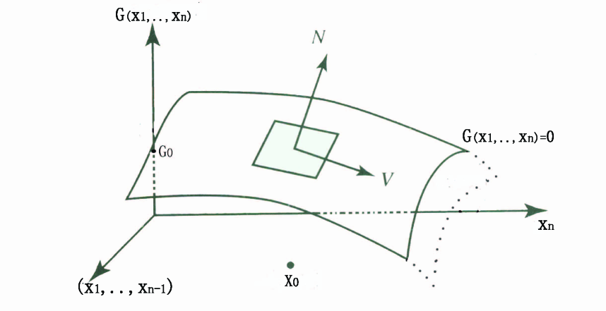
Figure 1: Local invariant manifold $M$ is represented by the equation $G(x_{1},\cdots,x_{n})=0$ in the $x_{1}\cdots x_{n}-$ space. Namely, $M$ is the intersection of the surface $G=G(x_{1},\cdots,x_{n})$ with the plane $G=0$ in $x_{1}\cdots x_{n}G-$space. Here $G(x_{1},\cdots,x_{n})$ is the solution of (82)-(83) via the method of characteristics. Note that $N=(u_{x_{1}},\cdots,u_{x_{n}},-1)$ and $V=(a_{1},\cdots,a_{n},c)$.

Relevance to predictability problem. When a SDE system starts to evolve inside a local almost sure invariant manifold $M$, it remains inside the manifold for a certain time period $0<t<T$. As determined above, this manifold holds solutions for the system, the time period $T$ may be taken as a lower bound of the predictability time scale.

7 Systems driven by non-Gaussian noise

Although Gaussian processes like Brownian motion have been widely used in modeling fluctuations in geophysical modeling, it turns out that many physical phenomena involve with non-Gaussian Levy motions. For instance, it has been argued that diffusion by geophysical turbulence [84] corresponds, loosely speaking, to a series of “pauses”, when the particle is trapped by a coherent structure, and “flights” or “jumps” or other extreme events, when the particle moves in the jet flow. Paleoclimatic data [20] also indicates such irregular processes.

Levy motions are thought to be appropriate models for non-Gaussian processes with jumps [79]. Let us recall that a Lévy motion $L(t)$ has independent and stationary increments, i.e., increments $\Delta L(t,\Delta t)=L(t+\Delta t)-L(t)$ are stationary (therefore $\Delta L$ has no statistical dependence on $t$) and independent for any non overlapping time lags $\Delta t$. Moreover, its sample paths are only continuous in probability, namely, ${\mathbb{P}}(|L(t)-L(t_{0})|\geq\delta)\to 0$ as $t\to t_{0}$ for any positive $\delta$. This continuity is weaker than the usual continuity in time.

This generalizes the Brownian motion $B(t)$, as $B(t)$ satisfies all these three conditions. But Additionally, (i) Almost every sample path of the Brownian motion is continuous in time in the usual sense and (ii) Brownian motion’s increments are Gaussian distributed.

SDEs driven by non-Gaussian Levy noises

$$dX_{t}=b(X_{t})dt+\sigma(X_{t})dL(t),$$ (85)

have attracted much attention [3, 42, 81] but this research subject is less developed. Recently, mean exit time estimates have been investigated by Imkeller et al [40, 41] and Yang and Duan [94].

Further progresses in SDEs driven by non-Gaussian noises will benefit the research in predictability in weather and climate systems with non-Gaussian (which is more common) model uncertainty.

8 Systems driven by colored noise

Colored noise, or noise with non-zero correlation in time, has been considered or used in the physical community [34, 31]. A good candidate for modeling colored noise is the fractional Brownian motion. A fractional Brownian motion (fBm) process $B^{H}$, where $H\in(0,1)$ is fixed, is still a Gaussian process. But it is characterized by the stationarity of its increments and a memory property. The increments of the fractional Brownian motion are not independent, except in the standard Brownian case ($H=\frac{1}{2}$). Thus it is not a Markov process except when $H=\frac{1}{2}$. Specifically, $B^{H}\left(0\right)=0$ and $Var\left[B^{H}\left(t\right)-B^{H}\left(s\right)\right]=\left|t-s\right|^{2H}$. It also exhibits power scaling and path regularity properties with Hölder parameter $H$, which are very distinct from Brownian motion. The standard Brownian motion is a special fBm with $H=1/2$.

The stochastic calculus involving fBm is currently being developed; see e.g. [64, 87] and references therein. This will lead to more advances in the study of SDEs driven by colored fBm noise:

$$dX_{t}=b(X_{t})dt+\sigma(X_{t})dB^{H}(t).$$ (86)

Since the fBM $B^{H}(t)$ is not Markov, the solution process $X_{t}$ is not Markov either. Thus the usual techniques from Markov processes will not be applicable to the study of SDEs driven by fBms. However, the random dynamical systems approach, as described in §3 above, looks promising [54]. The theory of RDS, developed by Arnold and coworkers [4], describes the qualitative behavior of systems of stochastic differential equations in terms of stability, Lyapunov exponents, invariant manifolds, and attractors.

Further progresses in SDEs driven by colored noises will benefit the research in predictability in weather and climate systems with more general (non-white noise) model uncertainty.

Acknowledgements.

This work was partly supported by the NSF Grants 0542450 and 0620539.

References

- [1] R. Abraham, J. E. Marsden and T. Ratiu. Manifolds, Tensor Analysis, and Applications. Second Ed., Springer-verlag, New York, 1988.
- [2] M. Allen,D. Frame, J. Kettleborough and D. Stainforth, Model error in weather and climate forecasting. Predictability of weather and climate (eds. Palmer, T. and Hagedorn, R.), pp. 391 428, Cambridge, UK: Cambridge University Press, 2006.
- [3] D. Applebaum. Lévy Processes and Stochastic Calculus. Cambridge University Press, Cambridge, UK, 2004.
- [4] L. Arnold. Random Dynamical Systems. Springer-Verlag, New York, 1998.
- [5] L. Arnold, Stochastic DifferentiL Equations, John Wiley & Sons, New York, 1974.
- [6] L. Arnold., Hasselmann’s program visited: The analysis of stochasticity in deterministic climate models. In J.-S. von Storch and P. Imkeller, editors, Stochastic climate models. pages 141–158, Boston, 2001. Birkhäuser.
- [7] J.-P. Aubin and G. Da Prato. Stochastic Viability and Invariance. Scuola Norm. Sup. Pisa, l27 (1990), 595-694.
- [8] P. S. Berloff, Random-forcing model of the mesoscale oceanic eddies. J. Fluid Mech. 529 (2005), 71-95.
- [9] L.C. Berselli, T. Iliescu and W. J. Layton. Mathematics of Large Eddy Simulation of Turbulent Flows. Springer Verlag, 2005.
- [10] D. Blomker and J. Duan, Predictability of the Burgers dynamics under model uncertainty. In Boris Rozovsky 60th birthday volume Stochastic Differential Equations: Theory and Applications, P. Baxendale and S. Lototsky (Eds.), p.71-90, World Scientific, New Jersey, 2007.
- [11] G. Boffetta, A. Celani, M. Cencini, G. Lacorata and A. Vulpiani, The predictability problem in systems with an uncertainty in the evolution law. J. Phys. A 33 (2000), 1313-1324.
- [12] G. Boffetta,M. Cencini, M. Falcioni and A. Vulpiani, Predictability: a way to characterize complexity. Phys. Rep. 356 (2002), no. 6, 367–474.
- [13] J. Brannan, J. Duan and V. Ervin, Escape Probability, Mean Residence Time and Geophysical Fluid Particle Dynamics, Physica D 133 (1999), 23-33.
- [14] T. Caraballo and J. Langa. A comparison of the longtime behavior of linear Ito and Stratonovich partial differential equations. Stochastic Anal. Appl., 19(2001), no.2 183-195.
- [15] P. Cessi and S. Louazel, Decadal oceanic response to stochastic wind forcing, J. Phys. Oceanography 31 (2001), 3020-3029.
- [16] A. Chorin, A. Kast and R. Kupferman. Unresolved computation and optimal predictions. Comm. Pure Appl. Math., 52 (1999), pp. 1231-1254.
- [17] H. Crauel and M. Gundlach (Eds.), Stochastic Dynamics. Papers from the Conference on Random Dynamical Systems held in Bremen, April 28–May 2, 1997. Springer-Verlag, New York, 1999.
- [18] G. Da Prato and J. Zabczyk, Stochastic Equations in Infinite Dimensions, Cambridge University Press, 1992.
- [19] T. DelSole. Stochastic models of quasigeostrophic turbulence. Surveys in Geophysics 25 (2004), 107-149.
- [20] P. D. Ditlevsen, Observation of stable noise induced millennial climate changes from an ice record. Geophys. Res. Lett. 26 (1999), 1441-1444.
- [21] A. Du and J. Duan, Invariant manifold reduction for stochastic dynamical systems. Dynamical Systems and Applications 16(2007), 681-696.
- [22] A. Du and J. Duan. A stochastic approach for parameterizing unresolved scales in a system with memory. Submitted, 2007.
- [23] J. Duan and B. Nadiga. Stochastic parameterization for large eddy simulation of geophysical flows. Proc. Amer. Math. Soc. 135 (2007), 1187-1196.
- [24] J. Duan, K. Lu and B. Schmalfuß. Invariant manifolds for stochastic partial differential equations. The Annals of Probability, 31(2003), 2109-2135.
- [25] J. Duan, K. Lu and B. Schmalfuß. Smooth stable and unstable manifolds for stochastic evolutionary equations. J. Dynamics and Diff. Eqns. 16 (2004), 949-972.
- [26] B. F. Farrell and P. J. Ioannou, Optimal perturbation of uncertain systems. Special issue on stochastic climate models. Stoch. Dyn. 2 (2002), no. 3, 395–402.
- [27] B. F. Farrell and P. J. Ioannou, Perturbation growth and structure in uncertain flows. I, II. J. Atmospheric Sci. 59 (2002), no. 18, 2629–2646, 2647–2664.
- [28] D. Filipovic. Invariant manifolds for weak solutions to stochastic equations. Probability Theory & Related Fields , Volume 118 (2000), Number 3. 323 - 341.
- [29] M. I. Freidlin and A. D. Wentzell, Random Perturbations of Dynamical Systems. 2nd Edition, Springer-Verlag, 1998.
- [30] J. Garcia-Ojalvo and J. M. Sancho, Noise in Spatially Extended Systems. Springer-Verlag, 1999.
- [31] C. W. Gardiner, Handbook of Stochastic Methods. Second Ed., Springer, New York, 1985.
- [32] A. Griffa and S. Castellari, Nonlinear general circulation of an ocean model driven by wind with a stochastic component. J. Marine Research, 49 (1991), 53-73.
- [33] J. Guckenheimer and P. Holmes. Nonlinear Oscillations,Dynamical Systems and Bifurcations of Vector Fields. Springer-Verlag, New York, 1983.
- [34] P. Hanggi and P. Jung, Colored Noise in Dynamical Systems. Advances in Chem. Phys., 89(1995),239-326.
- [35] K. Hasselmann, Stochastic climate models: Part I. Theory. Tellus, 28 (1976), 473-485.
- [36] G. Holloway, Ocean circulation: Flow in probability under statistical dynamical forcing, In Stochastic Models in Geosystems, S. Molchanov and W. Woyczynski (eds.), Springer-Verlag, New York, 1996.
- [37] W. Horsthemke and R. Lefever, Noise-Induced Transitions, Springer-Verlag, Berlin, 1984.
- [38] W. Huisinga, C. Schutte and A.M. Stuart, Extracting macroscopic stochastic dynamics: Model problems. Comm. Pure Appl. Math., 562003, 234-269.
- [39] P. Imkeller and A. Monahan (eds.), Conceptual Stochastic Climate Models. Special Issue:Stochastics and Dynamics, 2(2002),no.3.
- [40] P. Imkeller and I. Pavlyukevich, First exit time of SDEs driven by stable Lévy processes. Stoch. Proc. Appl. 116 (2006), 611-642.
- [41] P. Imkeller, I. Pavlyukevich and T. Wetzel, First exit times for Lévy-driven diffusions with exponentially light jumps. arXiv:0711.0982.
- [42] A. Janicki and A. Weron, Simulation and Chaotic Behavior of Stable Stochastic Processes, Marcel Dekker, Inc., 1994.
- [43] W. Just, H. Kantz, C. Rodenbeck and M. Helm, Stochastic modelling: replacing fast degrees of freedom by noise. J. Phys. A: Math. Gen., 34 (2001),3199–3213.
- [44] I. Karatzas and S. E. Shreve, Brownian Motion and Stochastic Calculus. Second Ed., Springer, New York, 1991.
- [45] V. M. Khade and J. A. Hansen, State dependent predictability: Impact of uncertainty dynamics, uncertainty structure and model inadequacies. Nonlinear Processes in Geophys. 11 (2004), 351-362.
- [46] F. C. Klebaner, Introduction to Stochastic Calculus with Applications. Imperial College Press, London, 2005.
- [47] R. Kleeman. Measuring dynamical prediction utility using relative entropy. J. Atmos Sci, 59:2057-2072, 2002.
- [48] P. E. Kloeden and E. Platen, Numerical solution of stochastic differential equations, Springer-Verlag, 1992; second corrected printing 1995.
- [49] H. Kunita. Stochastic flows and stochastic differential equations. Cambridge University Press, 1990.
- [50] C. E. Leith, Climate response and fluctuation dissipation, J. Atmos. Sci., 32 (1975), 2022-2025.
- [51] C. C. Lin and L. A. Segel, Mathematics Applied to Deterministic Problems in the Natural Sciences, SIAM, Philadelphia, 1988.
- [52] A. Majda, R. Kleeman and D. Cai, A mathematical framework for quantifying predictability through relative entropy. Special issue dedicated to Daniel W. Stroock and Srinivasa S. R. Varadhan on the occasion of their 60th birthday. Methods Appl. Anal. 9 (2002), no. 3, 425–444.
- [53] X. Mao. Stochastic differenntial equations & applications. Horwood Publishing, England, 1997.
- [54] B. Maslowski and B. Schmalfuss, Random dynamical systems and stationary solutions of differential equations driven by the fractional Brownian motion. Stochastic Anal. Appl. 22 (2004), no. 6, 1577–1607.
- [55] R.C McOwen. Partial Differential Equantions. Pearson Education, New Jersy, 2003.
- [56] A. Millet and P.-L. Morien, On implicit and explicit discretization schemes for parabolic SPDEs in any dimension. Stochastic Process. Appl. 115 (2005), no. 7, 1073–1106.
- [57] S.-E. A. Mohammed, T. Zhang and H, Zhao, The stable manifold theorem for semilinear stochastic evolution equations and stochastic partial differential equations, Memoirs of the American Mathematical Society, Vol. 196 (2008), pages 1-105.
- [58] M. Mu, W. S. Duan and B. Wang, Conditional nonlinear optimal perturbation and its applications. Nonlinear Processes in Geophys. 10 (2003), 493-501.
- [59] M. Mu, W. S. Duan and J. Chou, Recent advances in predictability studies in China (1999-2002). Adv. Atmos. Sci. 21 (2004), 437-443.
- [60] P. Müller, Stochastic forcing of quasi-geostrophic eddies, in Stochastic Modelling in Physical Oceanography, R. J. Adler, P. Müller and B. Rozovskii (eds.), Birkhäuser, 1996.
- [61] T. Naeh, M. M. Klosek, B. J. Matkowsky and Z. Schuss, A direct approach to the exit problem, SIAM J. Appl. Math. 50 (1990), 595-627.
- [62] C. Nicolis, Dynamics of Model Error: The Role of Unresolved Scales Revisited. Journal of the Atmospheric Sciences 61 (2004), 1740 1753.
- [63] G. R. North and R. F. Cahalan. Predictability in a solvable stochastic climate model. J. Atmos. Sci., 38:504–513, 1981.
- [64] D. Nualart, Stochastic calculus with respect to the fractional Brownian motion and applications. Contemporary Mathematics 336, 3-39, 2003.
- [65] B. Oksendal. Stochastic Differenntial Equations. Sixth Ed., Springer-Verlag, New York, 2003.
- [66] D. Orrell, L. Smith, J. Barkmeijer and T. N. Palmer, Model error in weather forecasting. Nonlinear Processes in Geophys. 8 (2001), 357-371.
- [67] D. Orrell, Role of the metric in forecast error growth: How chaotic is the weather? Tellus 54A (2002), 350-362.
- [68] T. N. Palmer and R. Hagedorn (eds.), Predictability of weather and climate, Cambridge, UK: Cambridge University Press, 2006.
- [69] T. N. Palmer, G. J. Shutts, R. Hagedorn, F. J. Doblas-Reyes, T. Jung and M. Leutbecher. Representing model uncertainty in weather and climate prediction. Annu. Rev. Earth Planet. Sci. 33 (2005), 163-193.
- [70] T. N. Palmer. A nonlinear dynamical perspective on model error: A proposal for non-local stochastic-dynamic parameterization in weather and climate prediction models. Q. J. Meteorological Soc. 127 (2001) Part B, 279-304.
- [71] C. Pasquero and E. Tziperman, Statistical parameterization of heterogeneous oceanic convection, J. Phys. Oceanography, 37 (2007), 214-229.
- [72] J. P. Peixoto and A. H. Oort, Physics of Climate. Springer, New York, 1992.
- [73] L. Perko. Differential Equations and Dynamical Systems. Cambridge University Press, 1990.
- [74] H. Risken, The Fokker-Planck Equation, Springer-Verlag, New York, 1984.
- [75] A. J. Roberts, A step towards holistic discretisation of stochastic partial differential equations. ANZIAM J. 45 (2003/04), (C), C1–C15.
- [76] B. L. Rozovskii, Stochastic Evolution Equations. Kluwer Academic Publishers, Boston, 1990.
- [77] R. M. Samelson, Stochastically forced current fluctuations in vertical shear and over topography, J. Geophys. Res. 94 (1989), 8207-8215.
- [78] R. Saravanan and J. C. McWilliams, Advective ocean-atmosphere interaction: An analytical stochastic model with implications for decadal variability, J. Climate 11 (1998), 165-188.
- [79] K.-I. Sato. Lévy Processes and Infinitely Divisible Distributions, Cambridge University Press, Cambridge, 1999.
- [80] T. Schneider and S. M. Griffies, A conceptual framework for predictability studies. J. of Climate 12 (1999), 3133-3155.
- [81] D. Schertzer, M. Larcheveque, J. Duan, V. Yanovsky and S. Lovejoy, Fractional Fokker–Planck Equation for Nonlinear Stochastic Differential Equations Driven by Non-Gaussian Levy Stable Noises. J. Math. Phys., 42 (2001), 200-212.
- [82] B. Schmalfuss, The random attractor of the stochastic Lorenz system. Zeitschrift f rangewandte mathematik und physik (ZAMP) 48 (1997), 951 - 975.
- [83] Z. Schuss, Theory and Applications of Stochastic Differential Equations, Wiley Sons, New York, 1980.
- [84] M. F. Shlesinger, G. M. Zaslavsky and U. Frisch, Lévy Flights and Related Topics in Physics (Lecture Notes in Physics, 450. Springer-Verlag, Berlin, 1995).
- [85] L. A. Smith, C. Ziehmann and K. Fraedrich, Uncertainty dynamics and predictability in chaotic systems. Q. J. R. Meteorol. Soc. 125 (1999), 2855-2886.
- [86] P. Sura and C. Penland, Sensitivity of a double-gyre model to details of stochastic forcing. Ocean Modelling, 4(2002), 327-345.
- [87] C.A. Tudor and F. Viens, Statistical aspects of the fractional stochastic calculus. Annals of Statistics, Vol. 35 (3) (2007), 1183-1212.
- [88] S. Vannitsem and Z. Toth, Short-term dynamics of model errors. J. Atmospheric Sci. 59 (2002), no. 17, 2594–2604.
- [89] W. Wang and J. Duan, A dynamical approximation for stochastic partial differential equations, J. Math. Phys. 48(2007), No. 10, 102701.
- [90] T. Wanner. Linearization of Random Dynamical Systems. Dynamics Report, Volumn 4. Spring-Verlog, New York, 1995.
- [91] E. Waymire and J. Duan (Eds.). Probability and Partial Differential Equations in Modern Applied Mathematics. Springer-Verlag, 2005.
- [92] D. S. Wilks, Effects of stochastic parameterizations in the Lorenz ’96 system. Q. J. R. Meteorol. Soc. 131 (2005), 389-407.
- [93] P. D. Williams. Modelling climate change: the role of unresolved processes. Phil. Trans. R. Soc. A (2005) 363, 2931-2946.
- [94] Z. Yang and J. Duan, Mean exit time estimates for dynamical systems with non-Gaussian Lévy noises. Preprint, 2008.
- [95] H. Zhao and Z. Zheng, Random periodic solutions of random dynamical systems. Preprint, 2008.