Large scale flow around turbulent spots

Abstract

Numerical simulations of a model of plane Couette flow focusing on its in-plane spatio-temporal properties are used to study the dynamics of turbulent spots. While the core of a spot is filled with small scale velocity fluctuations, a large scale flow extending far away and occupying the full gap between the driving plates is revealed upon filtering out small scales. It is characterized by streamwise inflow towards the spot and spanwise outflow from the spot, giving it a quadrupolar shape. A correction to the base flow is present within the spot in the form of a spanwise vortex with vorticity opposite in sign to that of the base flow. The Reynolds stresses are shown to be at the origin of this recirculation, whereas the quadrupolar shape of the in-plane flow results from the transport of this recirculation by the base flow that pumps it towards the spot in the streamwise direction and flushes it in the spanwise direction to insure mass conservation. These results shed light on earlier observations in plane Couette flow or other wall flows experiencing a direct transition to turbulence by spot nucleation.

1 Introduction

Being stable against infinitesimal perturbations for all Reynolds numbers, plane Couette flow (pCf), the shear flow between two parallel plates moving in opposite directions with velocity $\pm U_{\rm p}$, is the prototype of flows that require localized finite amplitude disturbances to be pushed towards a turbulent regime. The transition is thus characterized by the nucleation and nonlinear growth of domains of turbulent flow, separated from laminar flow by sharp fronts and called turbulent spots (e.g., [1, 2, 3, 4, 5]). This kind of transition is not restricted to pCf but is also present in plane Blasius (boundary layer) flow [6, 7] or plane Poiseuille flow [8]. A review of some relevant laboratory experiments is given by Henningson et al. [9] and of their numerical counterpart given by Mathew & Das [10]. In practice, direct transition to turbulence via spots can be expected whenever no low-Reynolds number instability of inertial origin exists, whereas turbulent solutions to the Navier–Stokes equations may exist and compete with the laminar base flow at moderate Reynolds number [11, Chap.6, §6.3].

Growing turbulent spots in pCf have been studied both experimentally [1, 2, 3, 4, 5] and numerically [12, 13, 14]. In their pioneering direct simulations of Navier–Stokes equations with realistic no-slip boundary conditions, Lundbladh & Johansson [12] pointed out that (i) the wall-normal velocity component —typical of internal irregular small scale structures— faded away outside the spot but (ii) slowly varying in-plane velocity components extended far outside with an inwards streamwise motion towards the spot at the streamwise edges and an outward spanwise motion at its spanwise edges. These observations were made by low-pass Gaussian filtering the small scales of the velocity field at mid-gap. Tillmark [5] confirmed them experimentally by detecting the outwards spanwise component that developed over the full gap between the plates.

More recently, Schumacher & Eckhardt [14] re-investigated the growth of turbulent spots by means of direct numerical simulations but using unrealistic free-slip boundary conditions at the plates. By averaging the flow field between the two plates, they also observed that the turbulent spot was accompanied by an overall spanwise outflow and streamwise inflow, which they termed quadrupolar.

Spots seem to behave as obstacles in the base flow [7, 15, 3]. Accordingly, they introduce additional pressure fields induced by the distribution of Reynolds stresses associated with the small scale fluctuations inside the spot and generating the large scale flows. A similar interpretation was put forward by Hayot & Pomeau [16] who introduced a back-flow to explain the organization of spiral turbulence in cylindrical Couette flow [17], with possible application to the banded turbulent regime discovered more recently in pCf [18] and numerically studied by Barkley & Tuckerman [19].

Previous experimental studies by Bottin et al. [20] have shown that, in the lowest part of the transitional Reynolds number range, flow patterns of interest extend over the full gap. We take advantage of this observation to study the dynamics of spots using numerical simulations of a previously derived model of pCf shown to display sufficiently good properties for this purpose [21]. The model is sketched in §2 and completed in the Appendix. Typical results of simulations are presented in §3 emphasizing the output of the filtering procedure: (i) the in-plane quadrupolar flow outside the spot and (ii) a spanwise recirculation cell inside. These observations are then interpreted in §4 where the generation of these two large scale flow components is explained in terms of Reynolds stresses averaged over the surface of the spot. In the concluding section, we summarize our results and point to their relevance to the interpretation of previous observations in other wall flows of less academical interest, such as plane Poiseuille [23] or Blasius flows [24].

2 The model

The model used here is an extension to realistic no-slip boundary conditions of an earlier model proposed by one of us [22] for unrealistic free-slip boundary conditions. It is derived in [21] from the Navier–Stokes equations through a systematic Galerkin method involving expansions in terms of polynomials, functions of the cross-stream coordinate $y$ multiplied by amplitudes describing the in-plane ($x,z$) space dependence of the full velocity field. The equations are written for the perturbation $(u^{\prime},v^{\prime},w^{\prime},p^{\prime})$ to the laminar basic flow $U_{\rm b}{\bf\hat{x}}$, where $\bf\hat{x}$ denotes the streamwise direction, i.e. $u=U_{\rm b}(y)+u^{\prime}$; $v^{\prime}$ and $w^{\prime}$ denote the perturbations in the cross-stream and spanwise directions, respectively, $p^{\prime}$ being the pressure perturbation. Lengths are scaled by the half-gap between the plates $h$, and velocities by $U_{\rm p}$ so that the time scale is $h/U_{\rm p}$. The control parameter is the Reynolds number defined as $R=U_{\rm p}h/\nu$, where $\nu$ is the fluid’s kinematic viscosity, and the dimensionless base flow profile reads $U_{\rm b}(y)=y$ for $y\in[-1,1]$.

In accordance with experimental observations [20], truncation of the Galerkin expansion at lowest consistent order is performed, reducing the set of basis functions to:

$$u^{\prime}(x,z,t,y) = U_{0}(x,z,t)B(1-y^{2})+U_{1}(x,z,t)Cy(1-y^{2}),$$ (1)

$$v^{\prime}(x,z,t,y) = V_{1}(x,z,t)A(1-y^{2})^{2},$$ (2)

$$w^{\prime}(x,z,t,y) = W_{0}(x,z,t)B(1-y^{2})+W_{1}(x,z,t)Cy(1-y^{2}),$$ (3)

where $A$, $B$, and $C$ are normalisation constants. These expressions are inserted in the continuity and Navier–Stokes equations, and projections of the results on the same basis functions using the canonical scalar product $\langle f,g\rangle=\int_{-1}^{+1}f(y)g(y)\,{\rm d}y$, are performed, which yields a set of coupled partial differential equations. For example, the projection of the continuity equation reads:

$$\partial_{x}U_{0}+\partial_{z}W_{0}=0\,,\quad\quad\partial_{x}U_{1}+\partial_{z}W_{1}=\beta\,V_{1}\,,$$ (4)

with $\beta=\sqrt{3}$. The complete model is given in the Appendix. Here we only display the equation for the amplitude $U_{0}$ of the streamwise velocity component which is even in $y$:

$$\partial_{t}U_{0}+N_{U_{0}}=-\partial_{x}P_{0}-a_{1}\partial_{x}U_{1}-a_{2}V_{1}+R^{-1}\left(\Delta-\gamma_{0}\right)U_{0}\,,$$ (5)

where $\Delta=\partial_{xx}+\partial_{zz}$ and with:

$$N_{U_{0}}=\alpha_{1}(U_{0}\partial_{x}U_{0}+W_{0}\partial_{z}U_{0})+\hbox{$1\over 2$}\alpha_{2}(U_{1}\partial_{x}U_{1}+V_{1}\beta^{\prime}U_{1}+W_{1}\partial_{z}W_{1})\,,$$ (6)

just to show that each equation has the form expected for a hydrodynamic problem. In particular, nonlinearities have the same structure as the classical advection term $\mathbf{v}\cdot\bm{\nabla}\mathbf{v}$. In the same way, the last term in (5), with the factor $R^{-1}$, accounts for the viscous dissipation associated with the cross-stream parabolic ($\gamma_{0}$) and in-plane dependencies of $U_{0}$. This flow component can straightforwardly be identified as the streamwise streak amplitude, so that the source term $-a_{2}V_{1}$ on the r.h.s. of (5) accounts for the lift-up mechanism since $V_{1}$ is the cross-stream velocity fluctuation. The physical role of the linear term $-a_{1}\partial_{x}U_{1}$ will be considered later.

On general grounds, the Reynolds–Orr equation governs the perturbation energy $E(t)=\frac{1}{2}\int_{\mathcal{V}}(u^{\prime 2}+v^{\prime 2}+w^{\prime 2})\,d\mathcal{V}$, where $\mathcal{V}$ is the volume of the domain. It can be symbolically written as $\frac{\rm d}{{\rm d}t}E=P-D$, where $P$ is the energy production issued from the interaction of the perturbation with the base flow $U_{\rm b}(y)\equiv y$, $P=-\int_{\mathcal{V}}u^{\prime}v^{\prime}\frac{\rm d}{{\rm d}y}U_{\rm b}\,d\mathcal{V}$, and $D$ is the dissipation due to viscous effects. In our model, one readily gets $P=-\int_{\mathcal{S}}\chi U_{0}V_{1}\,d\mathcal{S}$, where $\mathcal{S}$ is the surface of the domain and $\chi$ is a positive constant. Since $V_{1}$ generates $U_{0}$ through the lift-up mechanism, regions where the Reynolds stress $-U_{0}V_{1}$ is positive, thus destabilizing the base flow and contributing to the turbulence production, are those with $U_{0}>0$ and $V_{1}<0$ or the reverse, which obviously correspond to $Q_{2}$ and $Q_{4}$ events identified in the literature, see for example [25].

The main limitation of the model comes from its low order truncation. In fact, expressions (1–3) are only the first terms of series expansions and the derivation of models truncated at higher and higher orders remain possible. Up to now, this has not been done for several converging reasons, the main ones being that (i) the Reynolds number range we are interested in corresponds to the lower part of the pCf’s transitional regime where departures from laminar flow are known to occupy the full gap [20], (ii) $U_{1}$ already contains the lowest order non-trivial correction to the base flow thought to be important in the discussion of the laminar–turbulent coexistence [16]. Accordingly we believe that the lowest order model is sufficient to account for the large scale features present in the experiment at least at a qualitative level, the alternative being to turn to direct numerical simulations and not to consider a much more cumbersome higher order model. The discussion in §4 supports the validity our approach a posteriori.

3 Numerical simulations of turbulent spots

Our model was integrated on a rectangular $(x,z)$ domain with periodic boundary conditions, while being written for stream-functions $\Psi_{0}$, $\Psi_{1}$ and velocity potential $\Phi_{1}$ related to the velocity amplitudes through:

$$U_{0}=\widetilde{U}_{0}-\partial_{z}\Psi_{0}\,,\quad W_{0}=\widetilde{W}_{0}+\partial_{x}\Psi_{0}\,,$$ (7)

$$U_{1}=\widetilde{U}_{1}+\partial_{x}\Phi_{1}-\partial_{z}\Psi_{1}\,,\ W_{1}=\widetilde{W}_{1}+\partial_{z}\Phi_{1}+\partial_{x}\Psi_{1}\,,\ V_{1}=\Delta\Phi_{1}/\beta\,.$$ (8)

A standard, Fourier based, pseudo-spectral code was implemented with nonlinear terms and linear non-diagonal terms (e.g. $-a_{1}\partial_{x}U_{1}-a_{2}V_{1}$ in (5)) evaluated in physical space and integrated in time using a second order Adams–Bashforth scheme. The necessary introduction of $\widetilde{U}_{0}$,… is commented upon in the Appendix. Simulations were performed in a domain of size $(L_{x}\times L_{z})=(128\times 128)$ with effective space steps $\delta x=\delta z=0.25$ and $\delta t=0.01$. These values were retained as a good compromise between accuracy and the possibility to let sufficiently wide systems evolve over sufficiently large periods of time [21]. Concerning the accuracy problem, it should be noted that small-scale in-plane structures are pieces of streaks and streamwise vortices with typical size larger than 3, which makes more than 10 collocation points per structure. Smaller time steps did not produce results different from those shown here during comparable time lengths.

As an initial condition, we took localized expressions for $\Psi_{0}$, $\Psi_{1}$, and $\Phi_{1}$:

$$\Psi_{0}(x,z,t=0)=\Psi_{1}(x,z,t=0)=\Phi_{1}(x,z,t=0)=A\exp^{-(x^{2}+z^{2})/S}\,$$

where $A$ is an amplitude and $S$ is the size of the germ. Parameters $A=5$ and $S=2$ were found efficient in generating turbulent spots for $R=250$, well beyond $R_{\rm g}\sim 173$, above which sustained turbulence is expected in our model [21]. In practice, due to the highly unstable characteristics of the flow at such values of $R$, the apparent simplicity of the initial condition played no role after a few time units.

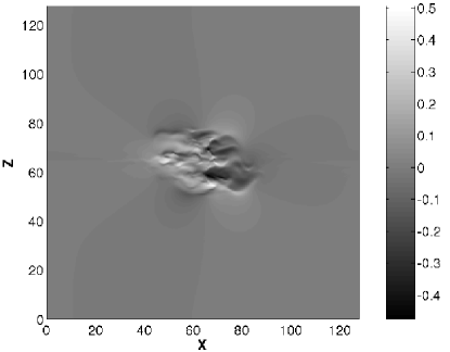
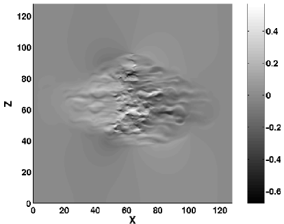
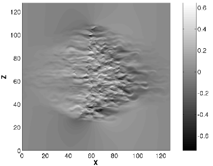
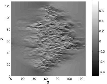
Figure 1: Growth of a turbulent spot at $R=250$ in a wide domain ($L_{x}\times L_{z}=128\times 128$). Field of amplitude $U_{0}(x,z,t)$ in gray levels at $t=50$, $150$, $250$ and $350$ (from left to right and top to bottom). The whole domain becomes uniformly turbulent at $t\approx 700$.

Spots are best illustrated by their most spectacular feature, namely their streamwise streaky structure [1, 2, 7, 8]. In turn, the latter is best visualized from the amplitude $U_{0}$ since streamwise streaks are easily identified as regions where $|W_{0}|\ll|U_{0}|$ alternating in the spanwise direction, and since $U_{0}$ is associated to velocity perturbations that are maximum in the mid-gap plane $y=0$. Figure 1 displays gray-level snapshots of $U_{0}$ at different times after launching. Denoting by $(x_{\rm C},z_{\rm C})$ the in-plane coordinates of the center of the spot we see that, contrasting with the cases of plane Poiseuille or boundary layer flows, the spot does not drift due to the absence of mean advection. One can also notice its overall ovoid shape with dominant negative values (dark gray) for $x>x_{\rm C}$ and positive values (light gray) for $x<x_{\rm C}$. Regions where $U_{0}$ is positive correspond to high and low speed streaks for $y>0$ and $y<0$, respectively, which compares well with the experimental observations in [20].

In the sequel, we study the state at $t=150$ but results and conclusions are identical at different times. The complete field $(U_{0},W_{0})$ corresponding to this reference state is displayed in Figure 2. Except in the very center of the spot that looks rather messy, streamwise structures are easily recognized but the trace of the large scale quadrupolar flow, of main concern in the present paper, is already visible.

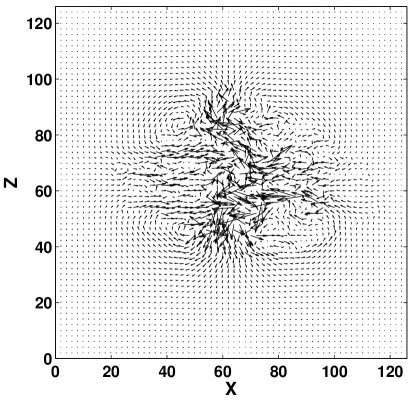
Figure 2: Streak flow field $(U_{0},W_{0})$ at $t=150$.

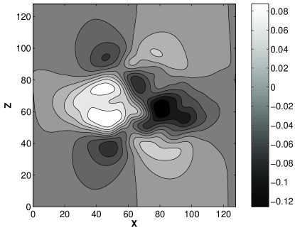
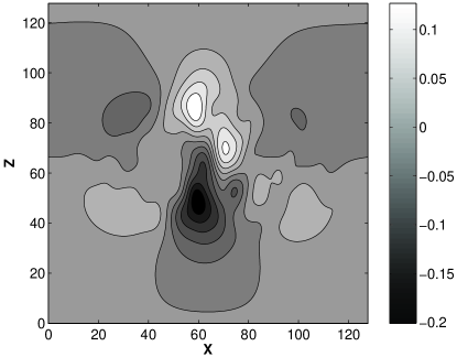
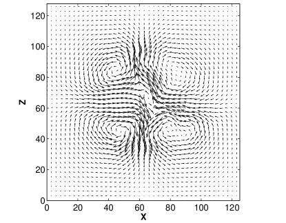
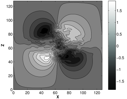
Figure 3: Top: level lines of averaged velocity components $\overline{U}_{0}$ (left) and $\overline{W}_{0}$ (right), illustrating large scale streamwise inflow and spanwise outflow around the spot. Bottom, left: representation of this flow as vectors. Bottom, right: level lines of the unfiltered stream function $\Psi_{0}$.

As done by Lundbladh & Johansson [12], we now proceed to the elimination of small scales using a Gaussian filter in spectral space:

$$\widehat{\overline{Z}}(k_{x},k_{z})=\widehat{Z}(k_{x},k_{z})\exp[-(k_{x}^{2}+k_{z}^{2})/(2\sigma)^{2}]\,,$$ (9)

where the hat denotes the Fourier transform of any quantity $Z=U_{0}$,…. In physical space, this corresponds to a convolution with a kernel $\propto\exp\left(-\sigma\sqrt{\zeta_{x}^{2}+\zeta_{z}^{2}}\right)$ where $\sigma$ is the parameter controlling the width of the domain over which the small scales are smoothed out by the operation. Small scales, indicated by superscript ‘s’, are recovered afterwards from the relation $Z^{\rm s}=Z-\overline{Z}$.

The diameter of the Gaussian averaging window has to be chosen in accordance with the size of the modulations to be eliminated, here the small scale streaks with spanwise wavelengths of the order $3$–$6$ as can be guessed from Figure 2. We used $\sigma=\pi/11$, but the results were found to be rather insensitive to this choice provided that $\sigma$ is sufficiently small.

As seen in Figure 3, this filtering procedure yields a clear picture of the flow outside the spot: the overall pattern formed by the in-plane components $\overline{U}_{0}$ and $\overline{W}_{0}$ has a quadrupolar aspect that could already be guessed from the consideration of the unfiltered stream-function $\Psi_{0}$ whose Laplacian is related to its vortical contents. In what follows, we term drift flow the large-scale velocity field $(\overline{U}_{0},\overline{W}_{0})$ with Poiseuille-like cross-stream profile by analogy with the case of Rayleigh–Bénard convection where a flow with the same global features was introduced by Siggia & Zippelius [26].

Figure 4 displays the velocity components associated to the fields $\Psi_{1},\Phi_{1}$. The distribution of the amplitude of $\overline{V}_{1}$, displayed in the left panel, represents an average wall-normal motion which is maximum in the mid-plane $y=0$, positive on the right of the spot’s center $x>x_{\rm C}$ and negative on its left. In turn, the flow $(\overline{U}_{1},\overline{W}_{1})$ shown in the right panel consists in a region centered around the spot where $|\overline{U}_{1}|\gg|\overline{W}_{1}|$ and $\overline{U}_{1}<0$. This structure is easily interpreted as a wide spanwise recirculation cell with vorticity opposite in sign to that of the base flow. It is further reminiscent of what can be deduced from DNS simulations of Lundbladh and Johansson [12], as displayed in seen their Fig. 9.

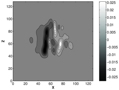
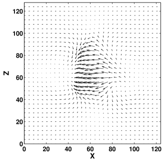
Figure 4: Velocity amplitudes $\overline{V}_{1}$ (left) and $(\overline{U}_{1},\overline{W}_{1})$ (right).

In Figure 5 (a) we display the profiles of $\overline{U}_{0}$ and $\overline{U}_{1}$ along a streamwise line going through the center of the spot. The dashed line corresponds to $\overline{U}_{0}$ and clearly points out the inwards character of the drift flow. In contrast, $\overline{U}_{1}$ (solid line) presents a deep trough at the location of the spot. At the spot’s center where $\overline{U}_{0}\simeq 0$, the superposition of the perturbation $u^{\prime}=\overline{U}_{1}Cy(1-y^{2})$ and the base flow $U_{\rm b}(y)\equiv y$, shown in Figure 5 (b), displays the characteristic S shape of the turbulent velocity profile expected for pCf. The presence of the spot thus locally increases the wall friction. At different positions inside the spot, where $\overline{U}_{0}\neq 0$ (and $\overline{W}_{0}\neq 0$), the full superposition $\overline{U}(y)=y(1+\overline{U}_{1}C(1-y^{2}))+\overline{U}_{0}B(1-y^{2})$ leads to asymmetric mean velocity profiles (Fig. 5(c) for point $x_{\rm L}$ and (d) for point $x_{\rm R}$) that are reminiscent of the averaged profiles obtained by Barkley & Tuckerman in their simulations of the banded regime of turbulent pCf [19].

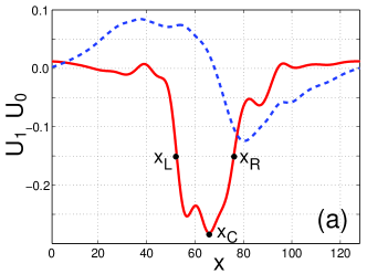
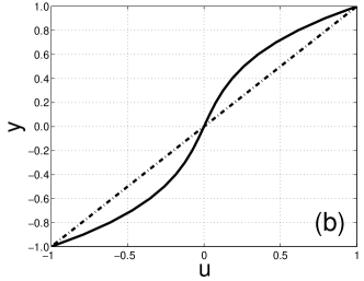
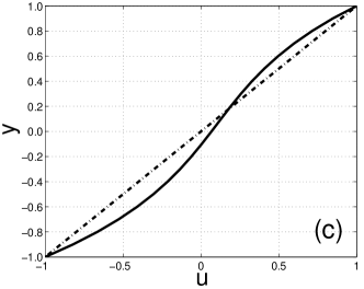
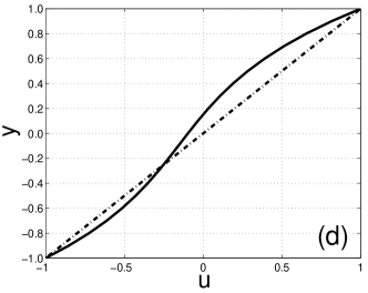
Figure 5: (a) $\overline{U}_{1}$ (red-solid) and $\overline{U}_{0}$ (blue-dashed) as functions of coordinate $x$ along the streamwise center-line. (b–d) Full average streamwise velocity profiles $\overline{U}(y)$ at $x=x_{\rm C}$ (b), $x=x_{\rm L}$ (c) and $x=x_{\rm R}$ (d); the laminar profile $U_{\rm b}(y)\equiv y$ is indicated by a dashed-dotted line.

4 Generation of large scales from small scales

The mechanism driving the quadrupolar drift flow is discussed in terms of equations obtained by filtering from the model’s equations, as described in the Appendix. We focus on the slowly varying quantities $A_{0}=\overline{\Delta\Psi}_{0}$, $A_{1}=\overline{\Delta\Psi}_{1}$, and $A_{2}=\overline{\Delta\Phi}_{1}$, driven by $B_{1}=-\xi\overline{{U_{0}^{\rm s}}{V_{1}^{\rm s}}}$ where $\xi=\alpha_{2}(\beta+\beta^{\prime\prime})>0$ and $B_{2}=\alpha_{1}\overline{({U_{0}^{\rm s}})^{2}-({W_{0}^{\rm s}})^{2}}+\alpha_{2}\overline{({U_{1}^{\rm s}})^{2}-({W_{1}^{\rm s}})^{2}}$. The latter quantities represent the components of the Reynolds stress tensor [27] which do not average to zero over the surface of the spot ($B_{1}$ corresponds to the energy extracted from the laminar flow and $B_{2}$ mostly to the energy contained in the streamwise streaks).

Introducing slow variables $X$ and $Z$ whose rate of change is inversely proportional to the width of the window that is dragged over the data upon averaging through (9), one can observe that, in the equations, the quantity $B_{1}$ appears with one derivative in $X$ or $Z$ less than $B_{2}$, due to the fact that $B_{1}$ substitutes one in-plane differentiation by a cross-stream $\mathcal{O}(1)$ differentiation. Further assuming that the spot is in a quasi-steady state ($\partial_{t}\approx 0$) and that space derivatives are negligible when compared to $\mathcal{O}(1)$ constants when operating on the same quantities, at lowest significant order one can simplify Equations (13–14) to read:

$$R^{-1}\gamma_{0}A_{0} = a_{1}\left(\hbox{$3\over 2$}\partial_{Z}A_{2}-\partial_{X}A_{1}\right)\,,$$ (10)

$$R^{-1}\gamma_{1}A_{1} = \partial_{Z}B_{1}-a_{1}\partial_{X}A_{0}\,,$$ (11)

$$R^{-1}\gamma_{1}A_{2} = -\partial_{X}B_{1}\,.$$ (12)

The structure of this system invites one to examine the shape of the dominant Reynolds stress contribution $B_{1}$ as a function of the slow variables. Figure 6 displays the averaged Reynolds stress field associated with the small scales $-\overline{{U_{0}^{\rm s}}{V_{1}^{\rm s}}}$. As could be anticipated the latter is positive under the spot and one can furthermore observe its single-humped shape that, following Li & Widnall [15] who developed a similar approach for spots in plane Poiseuille flow, can be modelled as a Gaussian function of the form $\exp[-(X^{2}+Z^{2})/2]$. This assumption will help us to make an educated guess about the mechanisms at work.

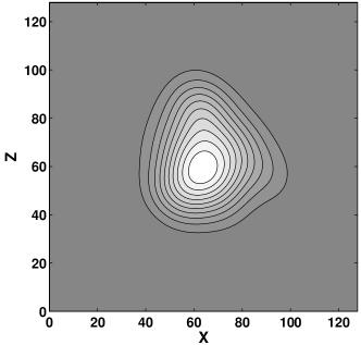
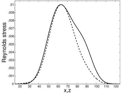
Figure 6: Distribution of the averaged Reynolds stress field $-\overline{{U_{0}^{\rm s}}{V_{1}^{\rm s}}}$ (left) and its variations along streamwise (solid line) and spanwise (dashed line) cuts through the maximum of the distribution taken as the center of the spot at $x_{\rm C}=64$, $z_{\rm C}=60$ (right).

Considering first Equation (12), from the third equation in (8), i.e. $V_{1}=\Delta\Phi_{1}/\beta$, we obtain that the contribution to $\overline{V}_{1}$ generated by $B_{1}$ is $\sim X\exp[-(X^{2}+Z^{2})/2]$, i.e. a pattern with a positive hump for $X>0$ and a negative one for $X<0$, resembling that in Figure 4 (left). This velocity component forms with $\overline{U}_{1}$ a large scale recirculation loop. As seen from the first equation in (8), $\overline{U}_{1}$ contains two contributions of potential and rotational origins, respectively. In the neighborhood of the $X$ axis, the variation of $\partial_{X}B_{1}$ is dominated by its $X$ dependence so that $A_{2}=(\partial_{XX}+\partial_{ZZ})\overline{\Phi}_{1}\approx\partial_{XX}\overline{\Phi}_{1}=-\partial_{X}B_{1}$ and, accordingly, $\partial_{X}\overline{\Phi}_{1}\sim-B_{1}\sim-\exp[-(X^{2}+Z^{2})/2]$. As to the rotational contribution $-\partial_{Z}\overline{\Psi}_{1}$, from (11) and forgetting the coupling with $A_{0}$ (which is of higher order owing to the way it is generated from $A_{1}$ and $A_{2}$), we have similarly $A_{1}=(\partial_{XX}+\partial_{ZZ})\overline{\Psi}_{1}\approx\partial_{ZZ}\overline{\Psi}_{1}\sim\partial_{Z}B_{1}$, hence $-\partial_{Z}\overline{\Psi}_{1}\sim-B_{1}$ so that it adds constructively to the potential part. The resulting $\overline{U}_{1}$ closes the recirculation loop as inferred from Figure 4 (right).

Inserting $A_{1}\sim\partial_{Z}B_{1}$ and $A_{2}\sim-\partial_{X}B_{1}$ in (10) we obtain a right hand side in the form $-XZ\exp[-(X^{2}+Z^{2})/2]$ for $\Delta\overline{\Psi}_{0}$ which is the vorticity contained in the $(U_{0},W_{0})$ velocity field. This field displays four lobes with alternating signs. An approximation to the large scale drift flow along the axes can easily be obtained. Indeed, $\overline{U}_{0}$ can be obtained from $\overline{U}_{0}=-\partial_{Z}\overline{\Psi}_{0}$ by integrating $A_{0}=(\partial_{XX}+\partial_{ZZ})\Psi_{0}$ over $Z$ and neglecting $\partial_{XX}\Psi_{0}$ since $\Psi_{0}$ varies much less with $X$ than with $Z$ along the $X$ axis. We obtain $\overline{U}_{0}\sim-X\exp[-(X^{2}+Z^{2})/2]$ which accounts for the observed inward flow along the streamwise center-line of the spot. The same argument can be transposed for the spanwise direction (now $\Psi_{0}$ varies most rapidly in the $X$ direction, which makes $\partial_{ZZ}\Psi_{0}$ negligible and eases the integration over $X$), yielding $\overline{W}_{0}\sim Z\exp[-(X^{2}+Z^{2})/2]$ which similarly accounts for the outward flow along the spanwise center-line. Notice however that this solution is too approximate to fulfil the continuity condition accurately since computing $\partial_{X}\overline{U}_{0}+\partial_{Z}\overline{W}_{0}$ leaves a residual of the form $(X^{2}-Z^{2})\exp[-(X^{2}+Z^{2})/2]$, though the main contribution in $\exp[-(X^{2}+Z^{2})/2]$ is nicely compensated near the origin where the Gaussian is at its maximum. At any rate the chosen shape is only a simplifying assumption.

Physically, the spot is thus characterized by a mean correction to the base flow (represented in the model by $\overline{U}_{1}<0$) itself generated by a wall normal velocity component (here $\overline{V}_{1}$) and forming a large recirculation loop. In turn, the transport of that mean correction (here $\overline{U}_{1}Cy(1-y^{2})$) by the base flow appears to be a source term for the large scale drift flow (here $(\overline{U}_{0},\overline{W}_{0})$) whose pattern is enslaved to its streamwise gradient, balancing viscous forces and inertia (according to $R^{-1}\gamma_{0}\overline{U}_{0}+a_{1}\partial_{x}\overline{U}_{1}\approx 0$) and expressing flow continuity ($\partial_{x}U_{0}+\partial_{z}W_{0}=0$).

5 Conclusion

In this paper, we have studied the large scale structure of the flow inside and around a turbulent spot in a transitional pCf model focusing on the in-plane dependence of a small number of velocity amplitudes [21]. The approach is supported by the qualitative consistency between previous experimental results in the transitional regime [20] and our own numerical simulations of the model.

Inside the spot, we find a wide spanwise recirculation loop with vorticity opposite in sign to that of the base flow. In particular, a patch of streamwise correction counteracting the base flow is observed, giving a S shape typical of turbulent flows to the velocity profile inside the spot. A reduced model (11–12) links this recirculation to Reynolds stresses $-\overline{{U_{0}^{\rm s}}{V_{1}^{\rm s}}}$ generated by the small scale fluctuations. Outside the spot, the existence of an inward-streamwise outward-spanwise quadrupolar drift flow has been pointed out, the origin of which is attributed to a linear coupling with this recirculation and linked to linear momentum conservation through (10). By simply assuming that the region where the Reynolds stresses contribute to the turbulent energy production (i.e. $-\xi\overline{{U_{0}^{\rm s}}{V_{1}^{\rm s}}}>0$) is one-humped with localized support, the main features of the large scale flow extracted from numerical simulations by filtering are recovered. In this approach, we only focused on the generation of large scales by small scales but considered neither (i) the interactions between small scales themselves nor (ii) the feedback of large scales on small scales. Closure assumptions are clearly needed in order to have a self-consistent theory, and especially to explain the sustainment of turbulence within a spot, problem (i), and its spreading as time proceeds, problem (ii).

Owing to the general character of the argument leading to their existence, one might also expect to find these large scale corrections in and around spots developing in transitional shear flows other than pCf for which they have already been accounted for [12, 14, 5]. Evidence of their presence can indeed be obtained from Figure 12 reporting numerical work of Henningson & Kim [23] on plane Poiseuille flow and from Figures 6 and 9 describing the result of ensemble averaging of turbulent spots in boundary layer flow with slightly adverse pressure gradient in the laboratory experiments of Schröder & Kompenhans [24]. Despite its limited cross-stream resolution, our modeling of transitional plane Couette flow has thus been shown to provide valuable explanations to previous observations, which might call for new laboratory experiments since, besides the theoretical challenge of understanding laminar–turbulent coexistence in detail, the problem of the transition to turbulence in wall flows has a great technical importance.

Appendix A Model’s equations and derivation of (10–12)

As explained in the main text, the model is obtained by projecting the Navier–Stokes equations on the chosen basis (1–3) with velocity perturbations expanded on the same basis. The set completing (4) and (5,6) reads:

$$\partial_{t}W_{0}+N_{W_{0}}=-\partial_{z}P_{0}-a_{1}\partial_{x}W_{1}+R^{-1}(\Delta-\gamma_{0})W_{0}\,,$$

$$N_{W_{0}}=\alpha_{1}(U_{0}\partial_{x}W_{0}+W_{0}\partial_{z}W_{0})+\alpha_{2}(U_{1}\partial_{x}W_{1}+W_{1}\partial_{z}W_{1}+\beta^{\prime}V_{1}W_{1})\,,$$

$$\partial_{t}U_{1}+N_{U_{1}}=\mbox{}-\partial_{x}P_{1}-a_{1}\partial_{x}U_{0}+R^{-1}(\Delta-\gamma_{1})U_{1}\,,$$

$$N_{U_{1}}=\alpha_{2}(U_{0}\partial_{x}U_{1}+U_{1}\partial_{x}U_{0}+W_{0}\partial_{z}U_{1}+W_{1}\partial_{z}U_{0}-\beta^{\prime\prime}V_{1}U_{0})\,,$$

$$\partial_{t}W_{1}+N_{W_{1}}=\mbox{}-\partial_{z}P_{1}-a_{1}\partial_{x}W_{0}+R^{-1}\left(\Delta-\gamma_{1}\right)W_{1}\,,$$

$$N_{W_{1}}=\alpha_{2}(U_{0}\partial_{x}W_{1}+U_{1}\partial_{x}W_{0}+W_{0}\partial_{z}W_{1}+W_{1}\partial_{z}W_{0}-\beta^{\prime\prime}V_{1}W_{0})\,,$$

$$\partial_{t}V_{1}+N_{V_{1}}=-\beta P_{1}+R^{-1}(\Delta-\gamma_{1}^{\prime})V_{1},$$

$$N_{V_{1}}=\alpha_{3}(U_{0}\partial_{x}V_{1}+W_{0}\partial_{z}V_{1})\,,$$

where $\Delta$ denotes the two-dimensional Laplacian $\partial_{xx}+\partial_{zz}$. Coefficients all derive from integrals of the form $J_{n,m}=\int_{0}^{1}y^{n}(1-y^{2})^{m}{\rm d}y=\sum_{k=0}^{m}{k\choose m}\frac{(-1)^{k}}{2k+n+1}$. We have: $a_{1}=1/\sqrt{7}$, $a_{2}=\sqrt{27/28}$, $\alpha_{1}=3\sqrt{15}/14$, $\alpha_{2}=\sqrt{15}/6$, $\alpha_{3}=5\sqrt{15}/22$, $\gamma_{0}=5/2$, $\gamma_{1}=21/2$, $\gamma_{1}^{\prime}=\beta^{2}$, $\beta^{\prime}=\frac{3}{2}\beta$, and $\beta^{\prime\prime}=\frac{1}{2}\beta$.

The equations governing fields $\Psi_{0}$, $\Psi_{1}$, $\Phi_{1}$, from which the velocity components derive through (7,8), are obtained in the usual way by differentiating and cross-subtracting or adding the previous equations. They read:

$$(\partial_{t}-R^{-1}(\Delta-\gamma_{0}))\Delta\Psi_{0}$$

$$\qquad=(\partial_{z}N_{U_{0}}-\partial_{x}N_{W_{0}})+a_{1}(\hbox{$3\over 2$}\partial_{z}\Delta\Phi_{1}-\partial_{x}\Delta\Psi_{1})\,,$$ (13)

$$(\partial_{t}-R^{-1}(\Delta-\gamma_{1}))\Delta\Psi_{1}$$

$$\qquad=(\partial_{z}N_{U_{1}}-\partial_{x}N_{W_{1}})-a_{1}\partial_{x}\Delta\Psi_{0}\,,$$ (14)

$$\left[\partial_{t}(\Delta-\beta^{2})-R^{-1}(\Delta^{2}-2\beta^{2}\Delta+\gamma_{1}\beta^{2})\right]\Delta\Phi_{1}$$

$$\qquad=\beta^{2}(\partial_{x}N_{U_{1}}+\partial_{z}N_{W_{1}})-\beta\Delta N_{V_{1}}\,.$$ (15)

The introduction of averaged quantities $\widetilde{U}_{0}$, $\widetilde{W}_{0}$, $\widetilde{U}_{1}$, and $\widetilde{W}_{1}$ in (7) and (8) is forced by our choice of periodic boundary conditions, otherwise the possibility of a uniform velocity correction corresponding to linearly increasing potential/stream functions would be overlooked. They are governed by:

$$\hbox{$\rm d\over{\rm d}t$}\widetilde{U}_{1} = \alpha_{2}(\beta+\beta^{\prime\prime}){\widetilde{U_{0}V_{1}}}-\gamma_{1}R^{-1}\widetilde{U}_{1}\,,$$

$$\hbox{$\rm d\over{\rm d}t$}\widetilde{W}_{1} = \alpha_{2}(\beta+\beta^{\prime\prime}){\widetilde{W_{0}V_{1}}}-\gamma_{1}R^{-1}\widetilde{W}_{1}\,$$

$$\hbox{$\rm d\over{\rm d}t$}\widetilde{U}_{0} = \alpha_{2}(\beta-\beta^{\prime}){\widetilde{U_{1}V_{1}}}-\gamma_{0}R^{-1}\widetilde{U}_{0}\,,$$

$$\hbox{$\rm d\over{\rm d}t$}\widetilde{W}_{0} = \alpha_{2}(\beta-\beta^{\prime}){\widetilde{W_{1}V_{1}}}-\gamma_{0}R^{-1}\widetilde{W}_{0}\,,$$

where the wide tildes mean averaging over the whole domain. Among this set of equations, the first one is the most relevant since it precisely corresponds to the expected mean flow correction. Quantity $\alpha_{2}(\beta+\beta^{\prime\prime})$ was denoted $\xi$ in the text.

It was observed in Figure 1 that the flow within the turbulent spot resembles developed turbulent flow, see also [9, 15]. Accordingly, one obtains that the only contributions to the averaged equations come from the terms that keep a constant sign over the surface of the spot, namely the main Reynolds stress term $-\overline{U_{0}V_{1}}$ associated with energy extraction from the mean flow and the other terms $\overline{U_{0}^{2}}$, $\overline{W_{0}^{2}}$, $\overline{U_{1}^{2}}$, and $\overline{W_{1}^{2}}$. Equations (13–14) then reduce to:

$$(\partial_{t}-R^{-1}(\Delta-\gamma_{0}))\Delta\overline{\Psi}_{0}$$

$$=\hbox{$1\over 2$}\partial_{xz}\left(\alpha_{1}\overline{U_{0}^{2}-W_{0}^{2}}+\alpha_{2}\overline{U_{1}^{2}-W_{1}^{2}}\,\right)+a_{1}\left(\hbox{$3\over 2$}\partial_{z}\Delta\overline{\Phi}_{1}-\partial_{x}\Delta\overline{\Psi}_{1}\right),$$ (16)

$$(\partial_{t}-R^{-1}(\Delta-\gamma_{1}))\Delta\overline{\Psi}_{1}=\partial_{z}\left(\,\overline{-\xi U_{0}V_{1}^{\phantom{2}}}\,\right)-a_{1}\partial_{x}\Delta\overline{\Psi}_{0}\,,$$ (17)

$$\left[\partial_{t}(\Delta-\beta^{2})-R^{-1}(\Delta^{2}-2\beta^{2}\Delta+\gamma_{1}\beta^{2})\right]\Delta\overline{\Phi}_{1}=\beta^{2}\partial_{x}\left(\,\overline{-\xi U_{0}V_{1}^{\phantom{2}}}\,\right),$$ (18)

with $\xi=\alpha_{2}(\beta+\beta^{\prime\prime})$. Following Li & Widnall, we then split the velocity components into small and large scales, i.e. $U_{0}\leadsto\overline{U}_{0}+U_{0}^{\rm s}$, etc., and only keep the contribution to the Reynolds stresses coming from the small scales. This leads to the same set of equations as above except that $U_{0}$, $U_{1}$, … are replaced by their small scale parts $U_{0}^{\rm s}$, $U_{1}^{\rm s}$, ….

References

- [1] N. Tillmark & P.H. Alfredsson, Experiments on transition in plane Couette flow, J. Fluid Mech. 235 (1992) 89–102.
- [2] F. Daviaud, J. Hegseth & P. Bergé, Subcritical transition to turbulence in plane Couette flow, Phys. Rev. Lett. 69 (1992) 2511–2514.
- [3] O. Dauchot & F. Daviaud, Finite amplitude perturbation in plane Couette flow, Europhysics letters. 28 (1994) 225–230.
- [4] O. Dauchot & F. Daviaud, Finite amplitude perturbation and spots growth-mechanism in plane Couette flow, Physics of Fluids. 7 (2), (1995) 335–343.
- [5] N. Tillmark, On the spreading mechanisms of a turbulent spot in plane Couette flow, Europhysics letters (1995)32 481–485.
- [6] H.W. Emmons, The laminar-turbulent transition in a boundary layer, Part I, J. Aero. Sci. 18 (1951) 490–498.
- [7] M. Gad-El-Hak, R.F. Blackwelder & J.J. Riley, On the growth of turbulent regions in laminar boundary layers, J. Fluid Mech. 110 (1981) 73–95.
- [8] D.R. Carlson, S.E. Widnall & M.F. Peeters, A flow visualization of transition in plane Poiseuille flow, J. Fluid Mech. 121 (1982) 487–505.
- [9] D.S. Henninson, A.V. Johansson & P.H. Alfredsson, Turbulent spots in channel flows, Journal of Engin. Math. 28 (1994) 21–42.
- [10] J. Mathew & A. Das, Direct numerical simulation of spots, Current Science 79 (2000) 816–820.
- [11] P. Manneville, Instabilities, Chaos and turbulence, Imperial College Press, 2004.
- [12] A. Lundbladh & A.V. Johansson, Direct simulation of turbulent spots in plane Couette flow, J. Fluid Mech. 229, (1991) 499–516.
- [13] A. Das & J. Mathew, Direct numerical simulation of turbulent spots, Computers & Fluids 30 (2001) 533–541.
- [14] J. Schumacher & B. Eckhardt, Evolution of turbulent spots in a parallel shear flow, Physical Review E 63 (2001) 046307.
- [15] F. Li & S.E. Widnall, Wave patterns in plane Poiseuille flow created by concentrated disturbances, J. Fluid Mech. 208 639–656 1989.
- [16] F. Hayot & Y. Pomeau, Turbulent domain stabilization in annular flows, Phys. Rev. E 50, (1994) 2019–2021.
- [17] D. Coles, Transition in circular Couette flow, J. Fluid Mech. 21 (1965) 385–425.
- [18] A. Prigent, G. Grégoire, H. Chaté, O. Dauchot & W. van Saarloos, Large-scale finite-wavelength modulation within turbulent shear flows, Phys. Rev. Lett. 89 (2002) 014501.
- [19] D. Barkley & L. Tuckerman, Mean Flow of Turbulent-Laminar Patterns in Plane Couette Flow, to appear in J. Fluid. Mech. (2007).
- [20] S. Bottin, O. Dauchot, F. Daviaud & P. Manneville, Experimental evidence of streamwise vortices as finite amplitude solution in transitional plane Couette flow, Phys. Fluids 10 (1998) 2597–2607.
- [21] M. Lagha, “Modeling the transition to turbulence in plane Couette flow,” PhD Thesis, Ecole Polytechnique, 2006.
- [22] P. Manneville, F. Locher, C.R. Acad. Sci. Paris 328 Serie IIb (2000) 159–164.
- [23] D.S. Henningson & J. Kim, On turbulent spots in plane Poiseuille flow, J. Fluid Mech. 228 (1991) 183–205.
- [24] A. Schröder & J. Kompenhans, Investigation of a turbulent spot using multi-plane stereo particle image velocimetry, Experiments in Fluids 36 (2004) 82–90.
- [25] Panton R.L, Overview of the self-sustaining mechanisms of wall turbulence, Progress in Aerospace Sciences 37 (2001) 341–383.
- [26] E.D. Siggia, A. Zippelius, Pattern selection in Rayleigh–B nard convection near threshold, Phys. Rev. Lett. 47 (1981) 835–838.
- [27] According to the LES terminology, these terms should rather be calledresidual stresses, see: S.B. Pope, Turbulent flows, Cambridge University Press, 2000, Ch. 13.