Chaotic advection of inertial particles in two dimensional flows

Abstract

We study the dynamics of inertial particles in two dimensional incompressible flows. The Maxey-Riley equation describing the motion of inertial particles is used to construct a four dimensional dissipative bailout embedding map. This map models the dynamics of the inertial particles while the base flow is represented by a $2-d$ area preserving map. The dynamics of particles heavier than the fluid, the aerosols, as well as that of bubbles, particles lighter than the fluid, can be classified into 3 main dynamical regimes - periodic orbits, chaotic structures and mixed regions. A phase diagram in the parameter space is constructed with the Lyapunov characteristic exponents of the $4-d$ map in which these dynamical regimes are distinctly identified. The embedding map can target periodic orbits, as well as chaotic structures, in both the aerosol and bubble regimes, at suitable values of the dissipation parameter.

I Introduction

The motion of inertial particles in fluids is governed by dynamical equations which display rich and complex behaviour. The inertial particles have density that is different from that of the fluid in which they are immersed, in contrast to the neutral particles which have the same density of the fluid. The dynamics of the inertial particles deserve attention from both the point of view of fundamental physics as they exhibit complex behaviour, as well as from that of their applicability to practical situations e.g. the transport of pollutants in the atmosphere and plankton in oceans mot03 ; reig01 ; babia00 ; cart02 ; benc03 ; raf06 .

If impurities in fluids are modeled by small spherical tracers, the Lagrangian dynamics of such small spherical tracers in two dimensional incompressible fluid flows is described by the Maxey-Riley equations. These are further simplified under various approximations to give a set of minimal equations called the embedding equations where the fluid flow dynamics is embedded in a larger set of equations which include the differences between the particle and fluid velocitiesmot03 ; cart02 . Although the Lagrangian dynamics of the underlying fluid flow is incompressible, the particle motion is compressible maxey87 , and has regions of contraction and expansion. The density grows in the former giving rise to clusters and falls in the latter giving rise to voids. The properties of the base flow have important consequences for the transport and mixing of particles. Map analogs of the embedding equations have also been constructed for cases where the fluid dynamics is modeled by area-preserving maps which essentially retain the qualitative features of the flow pierrehumbert00 ; fereday02 . The embedded dynamics in both cases is dissipative in nature.

Further complexity is added to the dynamics by the density difference between the particles and the fluid. In the case of two-dimensional chaotic flows, it has been observed earlier that particles with density higher than the base flow, the aerosols, tend to migrate away from the KAM islands, while particles lighter than the fluid, the bubbles, display the opposite tendency cartprl02 . Neutrally buoyant particles also showed a similar result, wherein the particles settled into the KAM islands. Our study indicates that in addition to the density difference, the dissipation parameter of the system also has an important role to play in the dynamic behaviour of the aerosols and the bubbles.

In Sec. II of this paper, the Maxey-Riley equation describing the motion of inertial particles is simplified to get a minimal equation of motion. A map analog of this minimal equation called the embedding map, is obtained to model the particle dynamics in discrete time. The fluid dynamics is represented by a $2-d$ base map, which we choose to be the standard map. The embedding map is four dimensional and dissipative, while the base map is two dimensional and area-preserving. Unlike the earlier results mentioned above, viz. that the bubbles tended to form structures in the KAM islandscartprl02 and the aerosols were pushed away, we found that structures form for both bubbles and aerosols in certain parameter regimes due to the role of the dissipation parameter. Both the aerosol and bubble regimes in the phase diagram show regions where periodic orbits as well as chaotic structures can be seen in the phase space plots. In Sec. III we obtain the phase diagram of the system in the $\alpha-\gamma$ space where $\alpha$ is the mass ratio parameter, and $\gamma$ is the dissipation parameter. The phase diagram shows rich structure in the $\alpha<1$ aerosol regime, as well as the $\alpha>1$ bubble regime. In addition to these, fully or partially mixed regimes can also be seen in both the aerosol and bubble cases. Thus the dynamic behaviour of the inertial particles can be of three major types. The Lyapunov exponents of the four dimensional map is used as the characterizers in demarcating these three major regimes. Our results can have implications for practical problems such as the dispersion of pollutants by atmospheric flows, and catalytic chemical reactions.

II The Embedding Equation

The motion of small spherical particles in an incompressible fluid has been studied extensively. The basic equation of motion was derived by Maxey and Riley maxey83 , and is given by babia00 ,

$$\begin{split}\rho_{p}\frac{d{\bf v}}{dt}&=\rho_{f}\frac{D{\bf u}}{Dt}+(\rho_{p}-\rho_{f}){\bf g}\\ &\quad-\frac{9\nu\rho_{f}}{2a^{2}}\left({\bf v}-{\bf u}-\frac{a^{2}}{6}\nabla^{2}{\bf u}\right)\\ &\quad-\frac{\rho_{f}}{2}\left(\frac{d{\bf v}}{dt}-\frac{D}{Dt}\left[{\bf u}+\frac{a^{2}}{10}\nabla^{2}{\bf u}\right]\right)\\ &\quad-\frac{9\rho_{f}}{2a}\sqrt{\frac{\nu}{\pi}}\int^{t}_{0}\frac{1}{\sqrt{t-\xi}}\frac{d}{d\xi}({\bf v}-{\bf u}-\frac{a^{2}}{6}\nabla^{2}{\bf u})\mathrm{d}\xi.\end{split}$$ (1)

Here ${\bf v}$ represents the particle velocity, ${\bf u}$ the fluid velocity, $\rho_{p}$ the density of the particle, $\rho_{f}$ the density of the fluid, and $\nu$, $a$, ${\bf g}$ represent the kinematic viscosity of the fluid, the radius of the particle and the acceleration due to gravity respectively.

The first term in the right of Eqn. 1 represents the force exerted by the undisturbed flow on the particle, the second term represents the buoyancy, the third term represents the Stokes drag, the fourth term represents the added mass, and the last the Basset-Bossinesq history force term. The derivative $D{\bf u}/Dt$ is taken along the path of the fluid element, $D{\bf u}/Dt={\partial u}/{\partial t}+({\bf u}\cdot\nabla){\bf u}$. The derivative $d{\bf u}/dt$, is taken along the trajectory of the particle $d{\bf u}/dt={\partial{\bf u}}/{\partial t}+({\bf v}\cdot\nabla){\bf u}$.

In deriving Eqn. 1 it was assumedmaxey83 ; babia00 that the particle radius, and the Reynolds number are small as well as the velocity gradients around the particle. It is also assumed that the initial velocities of the particle and the fluid are same. A full review of the problem can be found in Ref. michael97 .

Now Eqn. 1 can be simplified through the following arguments. The Faxen correction $a^{2}\nabla^{2}{\bf u}$ is of the magnitude $O(a^{2}u/L)$, and from the assumption, $a<<L$, this term’s contribution becomes negligible and can be excluded from the equation. The Basset history force term which takes into account viscous memory effects becomes less significant and can be dropped, as the particle size is sufficiently small and the concentration of particles is sufficiently low, that they do not modify the flow field or interact with each other benc03 ; michael97 . Under the low Reynolds number approximation , both the derivatives $D{\bf u}/Dt$ and $d{\bf v}/dt$ will approximately be the same maxey83 . We assume the buoyancy effects to be negligible. We thus arrive at the following equation,

$$\rho_{p}\frac{d{\bf v}}{dt} = \rho_{f}\frac{d{\bf u}}{dt}-\frac{9\nu\rho_{f}}{2a^{2}}({\bf v-u})-\frac{\rho_{f}}{2}\left(\frac{d{\bf v}}{dt}-\frac{d{\bf u}}{dt}\right).$$ (2)

This can be easily written into a non-dimensional form by proper rescaling of length, time and velocity by scale factors $L,T=L/U$ ,and $U$ respectively, to obtain,

$$\frac{d{\bf v}}{dt}-\alpha\frac{d{\bf u}}{dt} = -\frac{2}{3}\left(\frac{9\alpha}{2a^{2}Re}\right)({\bf v-u}),$$ (3)

where $\alpha=3\rho_{f}/(2\rho_{p}+\rho_{f})$ is the mass ratio parameter, $Re=(UL)/\nu$, is the Reynolds number of the fluid. By using the particle Stokes number $St=(2/9)a^{2}Re$ and defining the dissipation parameter as $\gamma=(2\alpha/3St)$, the final simplified equation takes the form,

$$\frac{d{\bf v}}{dt}-\alpha\frac{d{\bf u}}{dt} = -\gamma({\bf v-u}).$$ (4)

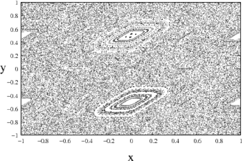
Figure 1: The phase space plot of the standard map for $K=2.0$. Random initial conditions distributed uniformly in the phase space were chosen.

The map analog of Eqn. 4 can be constructed. Let the base flow be represented by an area preserving map $M$ with the map evolution equation ${\bf x}_{n+1}={\bf M}({\bf x}_{n})$. As the particle dynamics in the fluid flow is compressible, it can be represented by a dissipative map. The map analog of Eqn. 4 has been chosen in mot03 to be,

$${\bf x}_{n+2}-{\bf M}({\bf x}_{n+1}) = e^{-\gamma}(\alpha{\bf x}_{n+1}-{\bf M}({\bf x}_{n})).$$ (5)

This equation can be rewritten by introducing a new variable $\delta$, which defines the detachment of the particle from the local fluid parcel as,

$${\bf x}_{n+1} = {\bf M(x}_{n})+{\bf\delta}_{n}$$

$${\bf{\delta}}_{n+1} = e^{-\gamma}[\alpha{\bf x}_{n+1}-{\bf M(x}_{n})].$$ (6)

This is the bailout embedding map. When the detachment measured by the $\delta$ is nonzero, the particle is said to have bailed out of the fluid trajectory. In the limit $\gamma\to\infty$ and $\alpha=1$, ${\bf\delta}\to 0$ and the fluid dynamics is recovered. So the fluid dynamics is embedded in the particle’s dynamics and is recovered under appropriate limit. This map is dissipative with the phase space contraction rate being $e^{-2a}$.

We choose the standard map chirikov , to be our base map $M$ as it is a prototypical area-preserving system and is widely studied in a variety of problems of both theoretical and experimental interest. The standard map serves as a test bed for various models regarding transport white98 . The map equation is given by,

$${\bf x}_{n+1} = {\bf x}_{n}+{\bf y}_{n+1}\ ~{}~{}~{}~{}~{}~{}~{}~{}~{}~{}~{}(Mod\ 1)$$

$${\bf y}_{n+1} = {\bf y}_{n}+\frac{K}{2\pi}\sin(2\pi{\bf x}_{n})\ ~{}~{}(Mod\ 1).$$ (7)

The parameter $K$ controls the chaoticity of the map. This map is taken to be the base map ${\bf M(x}_{n})$ in Eqn. (3). The phase space of the base standard map for $K=2.0$ is plotted in Fig. 1 in the region $x\in[-1,1],y\in[-1,1]$. The particle dynamics is governed by the 4 dimensional map ,

$$x_{n+1} = x_{n}+\frac{K}{2\pi}\sin(2\pi y_{n})+\delta_{n}^{x}$$

$$y_{n+1} = x_{n}+y_{n}+\frac{K}{2\pi}\sin(2\pi y_{n})+\delta_{n}^{y}$$

$$\delta_{n+1}^{x} = e^{-\gamma}[\alpha x_{n+1}-(x_{n+1}-\delta_{n}^{x})]$$

$$\delta_{n+1}^{y} = e^{-\gamma}[\alpha y_{n+1}-(y_{n+1}-\delta_{n}^{y})]$$ (8)

It is clear that this 4-dimensional map is invertible and dissipative. The embedding map has 3 parameters $K,\alpha,$ and $\gamma$. We plot the phase space portrait of the system evolved with random initial conditions at $K=2.0$. The phase space plot of the standard map at the same value of $K$ in Fig. 1 shows islands and chaotic regions separated by invariant tori which constitute barriers to transport. We plot the embedding map for the aerosol and the bubble cases, in Fig. 2. Unlike earlier studies which claim that only the aerosols are able to breach the invariant tori, we observe that that both the aerosols and bubbles have broken the barrier posed by the invariant curve and have targeted the islands forming periodic trajectories and structures. Thus, it is clear that the dissipation parameter $\gamma$ plays a vital role in the behaviour of both kinds of particles, the aerosols and the bubbles. Depending on particular values of $\gamma$ and $\alpha$ both these particles can form clusters or undergo mixing in the phase space. Therefore in order to identify the regimes in which clustering or mixing can take place, it is necessary to study the full phase diagram in the parameter space.

(a)

(b)

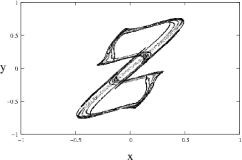
(c)

(d)

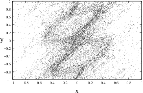
Figure 2: Phase space plots showing four different dynamical regimes of the embedding map.Here $K=2.0$ is fixed. (a) periodic trajectories ($\alpha=1.5,\gamma=0.7$), (b) chaotic structure ($\alpha=0.2$,$\gamma=0.9$), (c) full mixing ($\alpha=2.0$,$\gamma=0.9$)and (d) chaotic structure in a mixing background ($\alpha=0.7,\gamma=0.18$),

III The Phase Diagram

The phase diagram of the system can be constructed using the following criteria. The regimes where the largest Lyapunov characteristic exponent (LCE) $\lambda_{max}>0$ are regions of chaos and the regimes where $\lambda_{max}<0$ are regions of periodic behaviour. This property is used to identify the periodic regimes (marked in blue) in the phase diagram (see Fig. 3). A typical phase space plot in the periodic regime is shown in Fig. 2 (a). For the calculation of the Lyapunov exponent, the first 5000 iterates are taken as transients and the next 1000 iterates are stored, for 100 random initial conditions, uniformly spread in the phase space. We use the Gram-Schmidt reorthonormalization (GSR) procedure for the calculation of all the Lyapunov exponents of the embedded map wolf .

In the chaotic regimes, further classification can be carried out based on a scheme which uses the signs of the other Lyapunov exponents of the system and the occupation densities of the trajectories in the phase space. Fig. 4 shows all the Lyapunov exponents of the system for the dissipation $\gamma=0.7$ and $\alpha=0\to 3$. Chaotic structures in the phase space are found in the regimes where $\lambda_{2,3,4}<0$ while the largest LCE $\lambda_{1}$ (i.e.,$\lambda_{max}$) is greater than $0$. These are marked in green in the aerosol regions and yellow in the bubble regions in the phase diagram. For the regimes where both $\lambda_{1}$ and $\lambda_{2}$ greater than $0$, mixing is seen in the phase space.

Fig. 2 shows the phase space plots seen in three different dynamical regimes. Fig. 2(a) shows the periodic orbits in the bubble regimes ($\alpha=1.5,\gamma=0.7$). Here, both $\lambda_{1}$ and $\lambda_{2}$ are less than $0$. Chaotic structures are shown in Fig. 2(b) in the aerosol regime ($\alpha=0.2,\gamma=0.9$), where $\lambda_{1}>0$ and $\lambda_{2}<0$. The Figs. 2 (c),(d) show the mixing regimes for the bubble ($\alpha=2,\gamma=0.9$) and the aerosol ($\alpha=0.7,\gamma=0.18$) regimes respectively. In both the cases for the mixing regime, $\lambda_{1}$ and $\lambda_{2}$ are greater than $0$. We also note that the Lyapunov exponents $\lambda_{3}$ and $\lambda_{4}$ are less than $0$ in all the three regimes.

We see that the criterion based on the signs of Lyapunov exponents cannot distinguish between the phase space plots showing mixing regime (Fig. 2 (c)) and the chaotic structure in a mixing background (Fig. 2 (d)). Therefore we use the occupation densities to distinguish between these two cases.

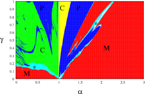
Figure 3: (Color Online) The phase diagram. The regimes with periodic structures are marked with P (blue). The regimes with chaotic structures are marked with C (green for aerosols and yellow for bubbles). The regimes with structures in a mixing background are marked with a ‘*’(light blue). The regimes with full mixing are marked with M (red).

The occupation densities in phase space can be calculated by covering the phase space by a $100\times 100$ mesh, and counting the number of boxes accessed by the iterates. The initial conditions and the transients are same as those that were used for calculating the Lyapunov exponent. The regions of parameter space where the iterates access more than $99\%$ of the phase space grid turn out to be fully mixing regions (marked in red in Fig. 3), with no remnant of any chaotic structure seen in the phase space plot, and have been marked with an M. The phase space plot of a mixing regime is seen in Fig. 2. The regions where the iterates access more than $90\%$ and less than $99\%$ of the boxes in the phase space are seen to contain a chaotic structure in a mixing background (marked with a ‘*’ - light blue in Fig. 3). Fig. 2 (d) shows the phase space plot of a chaotic structure in a mixing background.

Periodic structures are seen inside tongues in the parameter space in the aerosol as well as bubble regimes. Thus, the clustering or preferential concentration of inertial particles can be seen in both the aerosol and bubble regimes. Chaotic structures can be seen outside the tongues in the aerosol regime and in the border regions of the tongues in the bubble regime. The aerosol part ($0<\alpha<1$) of the phase diagram has a small region of mixing while the bubble part ($1<\alpha<3$) is dominated by the mixing regime. In recent work we reported nirmal that crisis induced intermittency is seen at some parameters in the aerosol regime in the phase diagram. Here the characteristic time between bursts scales algebraically with a function of the dissipation parameter $\gamma$, with the power law exponent to be $\beta=-1/3$.

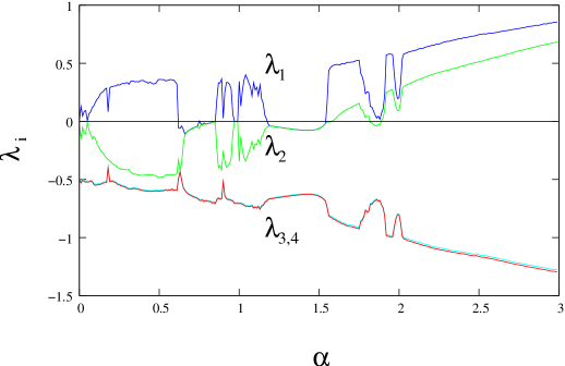
Figure 4: (Color Online) Four Lyapunov exponents of the embedding standard map; $K=2.0$ and $\gamma=0.7$. Intervals for which $\lambda_{1,2,3,4}<0$ have periodic orbits, and $\lambda_{2,3,4}<0$ have chaotic structures and $\lambda_{1,2}>0$ have mixing regimes in the phase space.

IV Conclusion

The present work discusses the Lagrangian dynamics of passive scalars of finite size in an incompressible two-dimensional flow for situations where the particle density can differ from that of the fluid. The motion of the advected particles is represented by a dissipative embedding map with the area preserving standard map as the base map.

The embedded standard map has three parameters, the nonlinearity $K$, the dissipation parameter $\gamma$ and the mass ratio parameter $\alpha$ which measures the extent to which the density of the particles differs from that of the fluid. The phase diagram of the system in the $\alpha-\gamma$ parameter space shows very rich structure with three types of dynamical behaviours - periodic orbits, chaotic structures, and mixed regimes which can be partially or fully mixed. The Lyapunov characteristic exponents (LCE) of the $4-d$ map are used to demarcate these dynamical regimes in the phase diagram. We observed that both aerols and bubbles can breach the invariant curves of the base map and form clusters, depending on the dissipation parameter of the system.

Our study can have implications for the preferential concentration of inertial particles in flows, as well as for the targeting of periodic structures. Earlier results for such systems indicated that bubbles could breach elliptic islands and target structures, whereas aerosols could not. Our results indicate that both aerosols and bubbles can breach the invariant curves of the base map and form clusters, depending on the dissipation parameter of the system. Mixing regimes can also exist for both aerosols and bubbles. Thus the dissipation parameter $\gamma$ plays as crucial role in clustering and mixing as does the density differential parameter $\alpha$, and the examination of the full phase diagram is necessary to draw conclusions about the parameter regimes where targeting and breaching can occur. These results can have implications for the dynamics of impurities in diverse application contexts, e.g. that of the dispersion of pollutants in the atmosphere, flows with suspended micro-structures, coagulation of material particles in flows, catalytic chemical reactions and the plankton population in oceans.

References

- (1) A.E. Motter, Y.C. Lai, and C. Grebogi, Phys. Rev. E 68, 056307(2003).
- (2) R. Reigada, F. Sagues,J.M. Sancho, Phys. Rev. E 64, 026307(2001).
- (3) A. Babiano, J.H.E. Cartwright, O. Piro, and A. Provenzale, Phys. Rev. Lett 84,5764 (2000).
- (4) J.H.E. Cartwright, M.O. Magnasco and O. Piro, Phys. Rev. E 65, 045203(R)(2002).
- (5) I.J. Benczik, Z. Toroczkai, and T. Tel, Phys. Rev. E 67, 036303 (2003).
- (6) R.D. Vilela, A.P.S. de Moura and C. Grebogi, Phys. Rev E 73, 026302(2006).
- (7) M.R. Maxey, J. Fluid Mech, 174, 441(1987).
- (8) R.T. Pierrehumbert, Chaos 10, 61(2000).
- (9) D.R. Fereday, P.H. Haynes, A. Wonhas and J.C. Vassilicos, Phys. Rev. E 65, 035301(R)(2002).
- (10) J.H.E. Cartwright, M.O. Magnasco, O. Piro, I. Tuval, Phys. Rev. Lett 89, 264501(2002).
- (11) M.R. Maxey, J.J. Riley, Phys. Fluids 26, 883(1983).
- (12) E.E. Michaelides, J. Fluids Eng. 119, 233 (1997).
- (13) B.V.Chirikov, Phys. Rep 52,265 (1979).
- (14) R.B. White, S. Benkada, S. Kassibrakis and G.M. Zaslavsky, Chaos 8, 757 (1998).
- (15) A. Wolf J. B. Swift, H. L. Swinney and J. A. Vastano, Physica D 16, 285 (1985).
- (16) N.N. Thyagu and N. Gupte, Phys. Rev. E 76, 046218 (2007).