STIRAP transport of Bose-Einstein condensate in triple-well trap

Abstract

The irreversible transport of multi-component Bose-Einstein condensate (BEC) is investigated within the Stimulated Adiabatic Raman Passage (STIRAP) scheme. A general formalism for a single BEC in M-well trap is derived and analogy between multi-photon and tunneling processes is demonstrated. STIRAP transport of BEC in a cyclic triple-well trap is explored for various values of detuning and interaction between BEC atoms. It is shown that STIRAP provides a complete population transfer at zero detuning and interaction and persists at their modest values. The detuning is found not to be obligatory. The possibility of non-adiabatic transport with intuitive order of couplings is demonstrated. Evolution of the condensate phases and generation of dynamical and geometric phases are inspected. It is shown that STIRAP allows to generate the unconventional geometrical phase which is now of a keen interest in quantum computing.

I Introduction

In recent decades, investigation of Bose-Einstein condensate (BEC) has become one of the main streams in modern physics (see for reviews and monographs Pit_Str_03 ; Petrick_Smith_02 ; Dalfovo_99 ; Leggett_01 ; Yuk_01 ; Pitaevskii_UFN_06 ; crossover ). In particular, a large attention is paid to dynamics of multi-component BEC and related coherent phenomena, e.g the Josephson effect in weakly bound BECs Yuk_JPA_96 -Opat_arXiv_08 .

Two kinds of multi-component BEC are usually considered. The first one is confined in a single trap and contains atoms in a few hyperfine levels (multi-level system or MLS). Here every component is formed by atoms in a given level. The components can be coupled by the laser light with the carrier frequency equal or close to the difference of the Bohr frequencies of the hyperfine states. One can control the coupling by varying parameters of the laser irradiation and so get different regimes of the transfer of atoms between the components: Josephson oscillations (JO), macroscopic quantum self-trapping (MQST), etc (see e.g. Raghavan_PRA_99 for discussion).

In the second kind of the multi-component BEC, the atoms are in the same hyperfine state but the trap is separated by laser-produced barriers into a series of weakly bound wells (multi-well system or MWS) arrays . BEC atoms can tunnel through the barriers and exhibit the similar effects as the MLS. In this case BEC components are represented by populations of the wells. Both MLS and MWS are obviously similar. Indeed, the coupling Rabi frequencies in MLS are counterparts of the barrier transition matrix elements in MWS. And detuning between Bohr and carrier frequencies in MLS is similar to detuning of the well depths in MWS. BEC in optical lattice Morsh_RMP_06 ; Yin_PR_06 can be also treated as MWS though, unlike a few-well traps arrays , the well depths and separations in optical lattices cannot be usually monitored individually for every cell.

Most of the studies consider BEC with two components Yuk_JPA_96 -Ne_lanl_08 and much less with three components Ne_lanl_08 -Opat_arXiv_08 . The later case is much more complicated. At the same time, it promises new dynamical regimes Nemoto_PRA_00 ; Zhang_PLA_01 and allows to consider not only linear (couplings 1-2, 2-3) but also cyclic (couplings 1-2, 2-3, 3-1) well chains.

In the present paper, we investigate BEC dynamics in the triple-well trap, i.e. MWS with the number of wells M=3. Unlike most of the previous studies, we will explore not oscillating fluxes of BEC but its complete and irreversible transport between the initial and target wells. For this aim, the coupling between BEC fractions (=components) will be monitored in time (unlike the constant coupling for the Josephson-like oscillations). Once being realized, BEC transport could open interesting perspectives in many areas, e.g. in exploration of coherent topological modes topol_1 ; Yuk_04 and diverse geometric phases Fuentes_PRA_02 -Balakrishnan_EPJD_06 . The later is especially important since geometric phases are considered as promising information carriers in quantum computing Nayak_RMP_08_gp ; Zhu_PRL_03_gp ; Feng_PRA_07_gp .

Due to similarity between MLS and MWS, one may try to apply for BEC transport numerous developments of modern quantum optics, in particular, adiabatic two-photon population transfer methods Vitanov . Between them the stimulated Raman adiabatic passage (STIRAP) Vitanov ; Berg seems to be the most suitable for our aims since it allows, at least in principle, the complete irreversible population transfer. The method was first developed for atoms and simple molecules Vitanov ; Berg and then probed in metal clusters Ne_PRA_04 -Ne_book_06 and variety of other systems, see references in Rab_PRA_08 . Quite recently STIRAP was applied to the transport of individual atoms Eckert_PRA_04 and BEC Graefe_PRA_06 ; Ne_lanl_08 ; Ne_Bars_08 ; Rab_PRA_08 ; Opat_arXiv_08 in the triple-well trap.

The applicability of STIRAP to BEC transport needs some care since interaction between BEC atoms results in a time-dependent nonlinearity of the problem, which can destroy the adiabatic transfer Graefe_PRA_06 ; Ne_Bars_08 ; Rab_PRA_08 ; Opat_arXiv_08 . This nonlinearity plays the same detrimental role as the dynamical Stark shift in electronic MLS systems, where it disturbs the two-photon resonance condition and thus breaks one of the basic STIRAP requirements (see discussion in Sec. II). As was shown in Graefe_PRA_06 , the undesirable nonlinear impact can be circumvented by using a detuning larger than the atomic interaction. The subsequent studies Rab_PRA_08 ; Opat_arXiv_08 confirmed that the detuning is useful if we aim a minimal (say $<1\%$) occupation of the intermediate well during STIRAP process. The less the (temporary) occupation, the better adiabaticity and robustness of the process. At the same time, one should recognize that occupation of the intermediate well cannot be fully avoided. Moreover, that occupation is temporal and in any case is further transferred to the final well. So it does not affect the final fidelity of the BEC transport.

In this study we will show that the robust and complete transport of the interacting BEC can take place even at zero detuning, regardless of the temporary weak population of the intermediate state. Of course such transport is more likely quasiadiabatic but we are interested in the transport completeness rather than in its purely adiabatic character. Moreover, we will show that the complete transfer can be done even at intuitive sequence of the pump and Stokes couplings (unlike their counterintuitive order in STIRAP), i.e. in strictly non-adiabatic case.

As compared with the previous studies Graefe_PRA_06 ; Rab_PRA_08 ; Opat_arXiv_08 , we will consider more general triple-well trap which has also 3-1 coupling and thus represents the circular configuration Ne_lanl_08 ; Ne_Bars_08 . Such configuration allows to run BEC through the circle as many rounds as we want and put it to any of three wells. Besides the populations, the condensate phases will be explored. Moreover, we will present some first examples of the dynamical and geometric phases generated in STIRAP. The later is possible because the circular well configuration and adiabatic STIRAP transfer allow to build the adiabatic cyclic evolution. It worth noting that condensate phases and their dynamical and geometric constituents were not yet explored in STIRAP (for exception of a brief phase analysis in Ne_Bars_08 ).

The paper is outlined as follows. In Sec. II we sketch STIRAP. In Sec. III a general mean-field formalism for dynamics of multi-component BEC is presented and specified for MWS with M=3. In Sec. IV the calculation scheme is given and similarity between our scenario and conventional STIRAP is discussed. In Sec. V results of the calculations are discussed. The conclusions are done in Sec. VI.

II STIRAP

STIRAP Vitanov ; Berg is the adiabatic two-step process providing the complete population transfer from the initial level $|1\rangle$ to the target level $|3\rangle$ via the intermediate level $|2\rangle$. Its scheme for MLS is illustrated in Fig. 1.

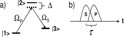
Figure 1: a) STIRAP scheme for a three-level $\Lambda$-system. The pump and Stokes pulses with Rabi frequencies $\Omega_{P}(t)$ and $\Omega_{S}(t)$ provide the couplings $|1\rangle-|2\rangle$ and $|2\rangle-|3\rangle$, respectively. $\Delta$ is the detuning from the intermediate level. b) Counterintuitive sequence of pump and Stokes pulses overlapping for a time $\tau$.

As is seen, the transfer is driven by the pump and Stokes laser pulses with Rabi frequencies $\Omega_{P}(t)$ and $\Omega_{S}(t)$. The pump laser couples the initial and intermediate states while the Stokes laser stimulates the emission from the intermediate state to the target one. In addition to the $\Lambda$-configuration given in the plot a), STIRAP can be also realized in the ladder and $\nu$-configurations Vitanov .

STIRAP has three principle requirements:
1) two-resonance condition for the laser carrier and Bohr frequencies

$$\omega_{P}-\omega_{S}=\omega_{3}-\omega_{1}$$ (1)

allowing a detuning $\Delta=(\omega_{2}-\omega_{1})-\omega_{P}=(\omega_{2}-\omega_{3})-\omega_{S}$ from $\omega_{2}$;
2) overlap of the pulses (during the time $\tau$) and their counterintuitive order (the Stokes pulse proceeds the pump one);
3) adiabatic evolution ensured by the condition

$$\Omega\tau>10$$ (2)

where $\Omega=\sqrt{\Omega_{P}^{2}+\Omega_{S}^{2}}$.

Due to interaction with the laser irradiation, the bare states $|1\rangle$, $|2\rangle$, $|3\rangle$ are transformed to the dressed states

$$|a^{+}\rangle = \sin\bar{\theta}\sin\bar{\phi}|1\rangle+\cos\bar{\phi}|2\rangle+\cos\bar{\theta}\sin\bar{\phi}|3\rangle,$$

$$|a^{0}\rangle = \cos\bar{\theta}|1\rangle-\sin\bar{\theta}|3\rangle,$$ (3)

$$|a^{-}\rangle = \sin\bar{\theta}\cos\bar{\phi}|1\rangle-\sin\bar{\phi}|2\rangle+\cos\bar{\theta}\cos\bar{\phi}|3\rangle$$

with the spectra

$$\omega^{\pm}=\Delta\pm\sqrt{\Delta^{2}+\Omega^{2}},\quad\omega^{0}=0$$ (4)

and mixing angle $\bar{\theta}$ determined through

$$\sin\bar{\theta}=\Omega_{P}/\Omega,\quad\cos\bar{\theta}=\Omega_{S}/\Omega.$$ (5)

The mixing angle $\bar{\phi}$, a known function of the Rabi frequencies and detuning Gaubatz_JCP_90 , is of no relevance in the present discussion. For the sake of simplicity, we omitted in this section time dependence of Rabi frequencies and other values.

STIRAP has been developed for population of non-dipole states (with the spin $J\neq 1$) which cannot be excited in the photoabsorption but can be reached by two dipole transitions via an intermediate state. The main aim was to avoid, as much as possible, the population of the intermediate state and thus prevent the leaking via decay of this state. As it is seen from Eq. (3), this can be achieved by keeping the system during all the process in the dressed state $|a^{0}\rangle$ which has no contribution from the intermediate state $|2\rangle$. For this aim we need an adiabatic evolution following with the counterintuitive sequence of the pump and Stokes pulses as is shown in Fig. 1b. In this case, we have $\Omega_{S}(t)\neq 0,\Omega_{P}(t)=0,\sin\bar{\theta}=0,\cos\bar{\theta}=1$ at early time and $\Omega_{S}(t)=0,\Omega_{P}(t)\neq 0,\sin\bar{\theta}=1,\cos\bar{\theta}=0$ at late time. Then, unlike $|a^{+}\rangle$ and $|a^{-}\rangle$, the state $|a^{0}\rangle$ is reduced to $|1\rangle$ at the beginning and to $|3\rangle$ at the end of the evolution. The main point is to evolve the system adiabatically, keeping it all the time in the state $|a_{0}\rangle$. As is seen from (2), for this aim we need either a strong coupling $\Omega$ (i.e. high laser intensities) or a long overlapping time $\tau$ which is just duration of the adiabatic evolution.

The STIRAP Hamiltonian reads

$$\bar{H}(t)=\frac{\hbar}{2}\left(\begin{array}[]{l}{\;\;0\qquad\Omega_{P}\qquad 0}\\ {\Omega_{P}\quad 2\Delta\quad\Omega_{S}}\\ {\;\;0\qquad\Omega_{S}\qquad 0}\end{array}\right).$$ (6)

Note that eqs. (3)-(6) are obtained in the rotating wave approximation (RWA). Using the fact that $\omega_{P,S},\omega_{1,2,3}\gg\Omega_{P,S},\Delta$, the RWA allows to omit the high laser and Bohr frequencies and keep only the low frequencies of interest.

Eqs. (3)-(6) also neglect the dynamical Stark shifts $\delta_{i}(t)$ pertinent to MLS, which are supposed here to be weak, $\delta_{i}(t)\ll\Omega_{P,S},\Delta$. Otherwise the shifts enter the diagonal terms in (6) and complicate Eqs. (3)-(5) Vitanov . The dynamical Stark shifts are detrimental for STIRAP since they destroy the two-resonance condition (1). The larger Rabi frequencies $\Omega_{P,S}$ (and hence the laser intensities), the stronger the Stark shifts. So, $\Omega_{P,S}$ must be large enough to keep the adiabatic condition (2) and, at the same time, small enough not to cause too strong Stark shifts. This problem is obviously absent in MWS. As was mentioned above, the time-dependent nonlinearity in BEC is detrimental for STIRAP Graefe_PRA_06 . In fact it plays the similar destructive role as the Stark shift.

III Mean-field description of BEC dynamics in MWS

We start from the non-linear Schr$\ddot{o}$dinger, or Gross-Pitaevskii equation GPE

$$i\hbar{\dot{\Psi}}({\vec{r}},t)=[-\frac{\hbar^{2}}{2m}\nabla^{2}+V_{ext}({\vec{r}},t)+g_{0}|\Psi({\vec{r}},t)|^{2}]\Psi({\vec{r}},t)$$ (7)

where the dot means time derivative, $\Psi({\vec{r}},t)$ is the classical order parameter of the system, $V_{ext}({\vec{r}},t)$ is the external trap potential involving both (generally time-dependent) confinement and coupling, $g_{0}=4\pi a/m$ is the parameter of interaction between BEC atoms, $a$ is the scattering length and $m$ is the atomic mass.

In what follows, we will consider the MWS where BEC is distributed between M wells separated by barriers. Then BEC components are reduced to the condensate fractions (=populations) in the wells. For BEC with weakly bound M fractions, the order parameter can be expanded as Raghavan_PRA_99

$$\Psi({\vec{r}},t)=\sqrt{N}\sum_{k=1}^{M}\psi_{k}(t)\Phi_{k}({\vec{r}})$$ (8)

where $\Phi_{k}({\vec{r}})$ is the static ground state solution of (7) for the isolated (without coupling) k-th well note and

$$\psi_{k}(t)=\sqrt{N_{k}(t)}e^{i\phi_{k}(t)}$$ (9)

is the amplitude related with the relative population $N_{k}(t)$ and corresponding phase $\phi_{k}(t)$ of the k-th fraction. The total number of atoms $N$ is conserved: $\int d\vec{r}|\Psi({\vec{r}},t)|^{2}/N=\sum_{k=1}^{M}N_{k}(t)=1\;.$

Being mainly interested in evolution of populations $N_{k}(t)$ and phases $\phi_{k}(t)$, we dispose by integration of the spatial distributions $\Phi_{k}({\vec{r}})$ and finally get Smerzi_PRL_97 ; Raghavan_PRA_99

$$i{\dot{\psi}}_{k}=[E_{k}(t)+UN|\psi_{k}|^{2}]\psi_{k}-\sum_{j\neq k}^{M}\Omega_{kj}(t)\psi_{j}\;$$ (10)

where

$$\Omega_{kj}(t)=-\frac{1}{\hbar}\int d{\vec{r}}\;[\frac{\hbar^{2}}{2m}\nabla\Phi^{*}_{k}\cdot\nabla\Phi_{j}+\Phi^{*}_{k}V_{ext}(t)\Phi_{j}]$$ (11)

is the coupling between BEC fractions,

$$E_{k}(t)=\frac{1}{\hbar}\int d{\vec{r}}\;[\frac{\hbar^{2}}{2m}|\nabla\Phi^{*}_{k}|^{2}+\Phi^{*}_{k}V_{ext}(t)\Phi_{k}]$$ (12)

is the potential depth, and

$$U=\frac{g_{0}}{\hbar}\int d{\vec{r}}\;|\Phi_{k}|^{4}\;$$ (13)

labels the interaction between BEC atoms. The values $\Omega_{kj}(t)$, $E_{k}(t)$, and $U$ have dimension of the frequency.

For simplicity we suppose that all the couplings have a common peak amplitude $K$. Then it is convenient to pick out this amplitude from the couplings

$$\Omega_{kj}(t)=K{\bar{\Omega}}_{kj}(t)$$ (14)

and scale (10) by $1/2K$ so as to get

$$i\dot{\psi}_{k}=[\bar{E}_{k}(t)+\Lambda|\psi_{k}|^{2}]\psi_{k}-\frac{1}{2}\sum_{j\neq k}^{M}\bar{\Omega}_{kj}(t)\psi_{j}\;.$$ (15)

Here

$$\bar{E}_{k}(t)=E_{k}(t)/2K,\quad\Lambda=UN/2K$$ (16)

and the time is scaled as $2Kt\to t$ thus becoming dimensionless. Eq. (15) is convenient since it is driven by one key parameter $\Lambda$ responsible for the interplay between the coupling and interaction. As is shown below, this parameter is decisive for STIRAP transport of BEC.

By substituting (9) into (15) and separating real and imaginary part, one gets equations describing evolution of the system in terms of fractional populations $N_{k}(t)$ and phases $\phi_{k}(t)$:

$${\dot{N}}_{k} = -\sum_{j\neq k}^{M}\bar{\Omega}_{kj}\sqrt{N_{j}N_{k}}\sin(\phi_{j}-\phi_{k})\;,$$ (17)

$${\dot{\phi}}_{k} = -[\bar{E}_{k}+\Lambda N_{k}]+\frac{1}{2}\sum_{j\neq k}^{M}\bar{\Omega}_{kj}\sqrt{\frac{N_{j}}{N_{k}}}\cos(\phi_{j}-\phi_{k}).$$ (18)

In MWS, the condensate is distributed between M space-shifted coupled wells, $V_{trap}(\vec{r})\to\sum_{k=1}^{M}V_{k}(\vec{r})$, with the depths $E_{k}$. The wells are separated by the barriers with penetrabilities $\Omega_{k\neq j}(t)$. We consider below a weak coupling between BEC fractions. Then only the neighbor fractions are coupled, $\Omega_{kj}\neq 0$ for $1\leq j=k\pm 1\leq M$, and interaction between atoms of different fractions can be neglected.

Equations (17)-(18) allow the classical analogy with the populations $N_{k}(t)$ and phases $\phi_{k}(t)$ treated as classical canonical conjugates. It is easy to verify that these equations can be casted in the canonical form

$${\dot{N}}_{k} = -\frac{\partial{\rm H}_{cl}}{\partial\phi_{k}}\;,$$ (19)

$${\dot{\phi}}_{k} = \frac{\partial{\rm H}_{cl}}{\partial N_{k}}$$ (20)

with the classical Hamiltonian

$${\rm H}_{cl}= - \sum_{k}^{M}(\bar{E}_{k}N_{k}+\frac{\Lambda N_{k}^{2}}{2})$$ (21)

$$+ \frac{1}{2}\sum_{kj}^{M}\bar{\Omega}_{kj}\sqrt{N_{k}N_{j}}\cos(\phi_{j}-\phi_{k})\;.$$

One may further upgrade (17)-(18) by means of canonical transformation of $N_{k}$ and $\phi_{k}$ to canonical pairs related to the population imbalances and phase differences. This will allow to remove from (17)-(18) the integral of motion $N$ and decrease the total number of equations from 2M to 2(M-1).

Let us consider the linear canonical transformation

$$z_{k}=\sum_{j}^{M}T_{kj}N_{j},\quad\theta_{k}=\sum_{j}^{M}R_{kj}\phi_{j}$$ (22)

with $z_{k}$ and $\theta_{k}$ being the population imbalances and phase differences, respectively. For the linear transformation, the matrices $T$ and $R$ in (22) are related as

$$R={\tilde{T}}^{-1}$$ (23)

i.e. the transformation matrix for the phases is the inverse transposed matrix for the populations.

For the MWS case with M=3 it is natural to chose

$$z_{1}=N_{2}-N_{1},\quad z_{2}=N_{3}-N_{2},\quad z_{3}=N\;.$$ (24)

Then one gets

$$T=\left(\begin{array}[]{ccc}-1&\;1&0\\ \;0&-1&1\\ \;1&\;1&1\\ \end{array}\right),\;R=\frac{1}{3}\left(\begin{array}[]{ccc}-2&\;1&1\\ -1&-1&2\\ \;1&\;1&1\\ \end{array}\right).$$ (25)

Matrices for the inverse transformation

$$N_{k}=\sum_{j}^{M}T^{-1}_{kj}z_{j},\quad\phi_{k}=\sum_{j}^{M}R^{-1}_{kj}\theta_{j}$$ (26)

for M=3 read

$$T^{-1}=\frac{1}{3}\left(\begin{array}[]{ccc}-2&-1&1\\ \;1&-1&1\\ \;1&\;2&1\\ \end{array}\right),\;R^{-1}=\left(\begin{array}[]{ccc}-1&\;0&1\\ \;1&-1&1\\ \;0&\;1&1\\ \end{array}\right).$$ (27)

New variables include the integral of motion $z_{3}=N$ and the total phase $\theta_{3}=\phi_{1}+\phi_{2}+\phi_{3}$. The equations for these values are straightforwardly separated from (17)-(18) and can be skipped. Then it is enough to solve the remaining four equations for $z_{1}$, $z_{2}$, $\theta_{1}$ and $\theta_{2}$.

Note that the formalism presented above is general and can be applied to both i) oscillating BEC fluxes in traps with constant parameters (like in Yuk_JPA_96 -Nista_08 and Nemoto_PRA_00 -Mossmann_PRA_06 ) and ii) irreversible BEC transport in traps with time-dependent parameters, e.g. $\Omega_{kj}(t)$. This formalism is partly given elsewhere Yuk_JPA_96 -Opat_arXiv_08 . However, we find useful to present here its full and consistent version.

Figure 2: a) The linear triple-well system containing the interacting BEC. The wells are denoted by the numbered circles. The tunneling couplings $\Omega_{12}(t)$ and $\Omega_{23}(t)$ are marked by double arrows. $E_{1}$, $E_{2}$ and $E_{3}$ are well depths. b) The circular configuration of triple-well system with the additional coupling 1-3. The solid lines connecting the circles mean the couplings. The dash curves represent the successive STIRAP transfers (1), (2) and (3), after which BEC returns back to the initial well $|1\rangle$. At every transfer only two couplings are active, as is shown in the plot a).

IV Calculation scheme for M=3

The triple-well system with interacting BEC and scheme of the cyclic STIRAP transport used in this study are depicted in Fig. 2. As is seen from the plot a), the adjoining wells are (weakly) coupled via the tunneling and the couplings $\Omega_{12}$ and $\Omega_{23}$ play the role of the pump $\Omega_{P}$ and Stokes $\Omega_{S}$ Rabi frequencies in a familiar STIRAP scheme in Fig 1a). Further, the plot b) shows that, compared with other STIRAP applications for the transport of individual atoms Eckert_PRA_04 and BEC Graefe_PRA_06 ; Rab_PRA_08 ; Opat_arXiv_08 , we implement here three STIRAP transfers, $|1\rangle\to|3\rangle$, $|3\rangle\to|2\rangle$ and $|2\rangle\to|1\rangle$, and every transfer follows the scheme a). In other words, these three transfers run via the intermediate states $|2\rangle$, $|1\rangle$, and $|3\rangle$ and use pairs of the couplings $(\Omega_{12},\Omega_{23})$, $(\Omega_{31},\Omega_{12})$ and $(\Omega_{23},\Omega_{31})$, respectively. As was mentioned above, we need three STIRAP steps to produce the cyclic evolution of the system and generate a geometric phase. Besides, this allows to test fidelity of STIRAP transport in the chain of transfers.

The similarity between the present scenario and typical STIRAP can be additionally justified by the comparison of their Hamiltonians. Following Fig. 2a), Eqs. (15) for M=3 can be written as

$$i\hbar{\dot{\psi}}_{k}(t)=H(t){\psi}_{k}(t)$$ (28)

with the Hamiltonian

$$H(t)=\left(\begin{array}[]{l}{\bar{E}_{1}+A_{1}(t)\quad\;\;\Omega_{P}(t)\quad\quad\quad\quad 0}\\ {\quad\Omega_{P}(t)\quad\quad\bar{E}_{2}+A_{2}(t)\;\;\quad\Omega_{S}(t)}\\ {\quad 0\quad\qquad\quad\quad\Omega_{S}(t)\quad\quad\bar{E}_{3}+A_{3}(t)}\end{array}\right)\;$$ (29)

where $A_{k}(t)=\Lambda N_{k}(t)$ is the non-linear interaction contribution and $\Omega_{P}(t)=-\bar{\Omega}_{12}(t)/2$ and $\Omega_{S}(t)=-\bar{\Omega}_{23}(t)/2$ are the pump and Stokes couplings. The nonlinear terms $A_{k}(t)$ are detrimental for adiabatic transfer within STIRAP Graefe_PRA_06 . If to omit them, then (29) fully coincides with STIRAP Hamiltonian (6).

In our study the time-dependent part of the coupling (14) has the Gauss form

$${\bar{\Omega}}_{kj}(t)=\exp\{-\frac{(t_{kj}-t)^{2}}{\Gamma^{2}}\}$$ (30)

where $t_{kj}$ and $\Gamma_{kj}$ are centroid and width parameters. This form is smooth which is important for adiabaticity of the process.

Using (14) and (30) one may amend the STIRAP adiabatic condition (2). Following Vitanov ; Messia one gets

$$\frac{\Omega_{S}\dot{\Omega}_{P}-\Omega_{P}\dot{\Omega}_{S}}{\Omega^{3}}\ll 1\;\mbox{or}\;\Omega_{\tau}\gg\frac{|d|}{\sqrt{2}\;\Gamma^{2}}$$ (31)

where $\Omega_{\tau}$ is the average amplitude of the pump and Stokes couplings during the overlap time $\tau$ and $d=t_{12}-t_{23}$ is the relative pump-Stokes shift. Usually one may take $\Omega_{\tau}\approx 0.5K$ and $\tau\approx\Gamma$. Then (31) is cast to

$$K\tau^{2}\gg\sqrt{2}|d|$$ (32)

which means that STIRAP needs a strong coupling amplitude $K$ and/or a long overlap time $\tau$. It is easy to see that (32) remains to be the same for the scaled dimensionless time.

Since we use the mean-field approximation, the number of atoms in BEC should be sufficiently large to neglect the quantum corrections. In the present study we suppose that $N>10^{4}$ Smerzi_PRL_97 ; Raghavan_PRA_99 . The total number of atoms is included to the parameter $\Lambda$ in (16).

V Results and discussion

V.0.1 Populations and phases

Results of the calculations are depicted in Figs. 3-6. In all the figures time is dimensionless. The coupling parameters are $\Gamma$ = 5.4 and $d$ = -5. Then for $K=1$ we get $K\Gamma^{2}\approx$ 30 and $\sqrt{2}|d|\approx$ 7 and so keep the adiabatic condition (32).

In Fig. 3 the populations $N_{i}(t)$ during three STIRAP steps are exhibited. The calculations are performed at initial conditions (t=0) $N_{1}=1,\;N_{2}=N_{3}=0$ and $\phi_{1}=\phi_{2}=\phi_{3}=0$. The sequence of the pairs of Stokes (first) and pump (second) couplings is given in the panel a) while other plots demonstrate evolution of $N_{i}(t)$ at different values of the ratio $\Lambda$ and detuning $\Delta$.

As is seen from the panel b), all three STIRAP steps are robust and complete for $\Lambda=\Delta=0$, i.e. without interaction $U$ and detuning. The minor peaks observed at t=20, 80 and 140, i.e. during the transfers, mean a weak temporary population of the intermediate wells, which hints that the transport is not fully adiabatic. However, what is important for our aims, the transport is complete. And this takes place even after 3 STIRAP steps and despite deviations (though minor) from adiabaticity.

Figure 3: STIRAP transport of BEC in the circular well chain. a): Sequence of the pairs of Stokes (first) and pump (second) couplings $\Omega_{kj}$ responsible for 1-2 (solid line), 2-3 (dash line) and 2-3 (dotted line) couplings. b)-h): Evolution of the populations $N_{1}$ (solid line) $N_{2}$ (dash line), and $N_{3}$ (dotted line) at different values of the ratio $\Lambda$ and detuning $\Delta$.

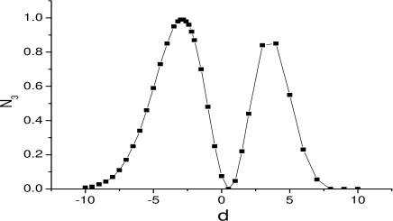
Figure 4: Population $N_{3}$ at different relative shift $d$ between pump and Stokes couplings. The maximal populations at counterintuitive $(d<0)$ and intuitive $(d>0)$ coupling order correspond to STIRAP and non-adiabatic transport.

The next panels c)-e) show that switching on the interaction worsens the transport. The damage is negligible for $\Lambda=0.1$ and does not exceed 20$\%$ for $\Lambda=\pm 0.2$ but STIRAP ruins for larger interaction (not shown). In any case, STIRAP is robust under a modest interaction and this holds without any detuning. The comparison of the cases d) and e) shows that the result somewhat depends on the interaction sign.

The remaining three panels f)-h) demonstrate role of detuning in the non-interacting condensate ($\Lambda=0$). It is seen that a considerable detuning spoils the transport and the result slightly depends on the detuning sign. Our calculations generally confirm that a weak detuning is not harmful and, in accordance with Graefe_PRA_06 ; Rab_PRA_08 ; Opat_arXiv_08 , may be even useful to amend slightly adiabaticity of the process. However, the detuning is obviously not obligatory. Moreover, in real conditions, the adiabaticity is never fully kept. Nevertheless, the adiabatic transport schemes should work if diabatic perturbations are not strong, which is confirmed by our results.

In Fig. 4 the dependence of the transport on the relative shift $d$ of the pump and Stokes couplings is demonstrated. The results are obtained for $\Lambda=\Delta=0$ and $\Gamma$=4.36. Both counterintuitive (Stokes precedes pump, $d<0$) and intuitive (pump precedes Stokes, $d>0$) sequences of the couplings are covered. It is seen that the best result (complete transport) takes place for the counterintuitive order, $d=-3$, pertinent for STIRAP. The intuitive order also leads to the appreciable population, $N_{3}\sim 80-90\%$ at $d=3$, though this transfer is not adiabatic. What is remarkable, there is no any transfer without the shift, i.e. for $d=0$. Being adiabatic, STIRAP transfer is less sensitive to the parameters of the process and so is more preferable than its non-adiabatic counterpart. This is partly confirmed by Fig. 4 where the left adiabatic peak is broader than the right non-adiabatic one, hence less sensitivity to the shift $d$.

In Fig. 5 the phases $\phi_{i}$ and phase differences $\theta_{i}$ are given for the cases with and without the interaction $U$. It is seen that the interaction and corresponding non-linear effects drastically change both $\phi_{i}$ and $\theta_{i}$. This conclusion generally agrees with the observations for the oscillating BEC Smerzi_PRL_97 ; Raghavan_PRA_99 where the interaction also strongly affects the phases. So the interaction can in principle be implemented (via the Feshbach resonance) to control geometric phases generated during BEC transport.

V.1 Geometric phases

Figure 5: Phases $\phi_{i}$ (i=1,2,3, left panels) and phase differences $\theta_{i}$ (i=1,2, right panels) calculated without ($\Lambda=0$, upper panels) and with ($\Lambda=0.2$, bottom panels) interaction. In all the panels $\Delta=0$. For i=1,2,3 the solid, dash, and dotted lines are used. The phases in the upper and bottom panels correspond to the populations in Figs. 3b) and 3d), respectively.

Figure 6: Total $\gamma_{t}$ (solid line), dynamical $\gamma_{d}$ (dash line), and geometric $\gamma_{g}$ (dotted line) phases for the cases without (a) and with (b) interaction $U$. In both panels $\Delta=0$. In the panel a) the unconventional geometric phase $\gamma_{g}=\alpha\gamma_{d}$ with $\alpha\neq-1$ is obtained.

Being coherent, BEC provides an interesting possibility to generate and investigate various geometric (topological) phases $\gamma_{g}$ Fuentes_PRA_02 -Balakrishnan_EPJD_06 . These phases are known to be mainly determined by the path topology (unlike the dynamical phases $\gamma_{p}$ which depend on the process rate as well), see e.g. Mukunda . Because of this feature, $\gamma_{g}$ is less sensitive to parameters of the process and so can serve as a reliable carrier of information Nayak_RMP_08. During last decades implementation of geometric phases in the so called geometric quantum computation has become actual Nayak_RMP_08_gp ; Zhu_PRL_03_gp ; Feng_PRA_07_gp . In this connection using BEC transport for exploration of various $\gamma_{g}$ could be indeed of a keen interest.

The geometric phases in BEC dynamics have been already studied elsewhere Fuentes_PRA_02 -Balakrishnan_EPJD_06 . However, these studies concerned the oscillating BEC and, by our knowledge, still nothing was done for $\gamma_{g}$ in BEC transport problems.

In principle, geometrical and dynamical phases in the oscillation and transport dynamics can be described within the same general formalism given in Mukunda . In the present study, we exploit its version Balakrishnan_EPJD_06 . There, for the cyclic evolution during the time interval $t=[0,T]$, the geometric phase is determined as the difference between the total and the dynamical phases

$$\gamma_{g}=\gamma_{t}-\gamma_{d}$$ (33)

where

$$\gamma_{t} = \mbox{arg}\;(\vec{\psi}(0)\cdot\vec{\psi}(T))\;,$$ (34)

$$\gamma_{d} = \mbox{Im}\int^{T}_{0}dt(\vec{\psi}(t)\cdot\dot{\vec{\psi}}(t))\;,$$ (35)

and

$$\vec{\psi}(t)=(\psi_{1}(t),\psi_{2}(t),\psi_{3}(t))$$ (36)

is the state vector consisting of the components (9) of the condensate.

In Fig. 6 results of our calculations of $\gamma_{t}$, $\gamma_{d}$, and $\gamma_{g}$ for the three-step STIRAP transport are presented. Due to a cyclic adiabatic evolution, the Berry phase Berry is produced. The cases with and without interaction (corresponding to the protocols of Figs. 3b), 3d) and 5) are considered. It is seen that in both cases we observe proportionality of the geometric and dynamical phases, $\gamma_{g}\approx\alpha\gamma_{d}$. However, for $\Lambda=0.2$ there is a large mutual compensation of the phases ($\alpha\approx-1$) thus giving $\gamma_{t}\approx 0$. Instead for $\Lambda=0$ $\alpha\approx-2$ (for $t>90$) and we gain the so called unconventional geometric phase Zhu_PRL_03_gp . This gives a chance to determine $\gamma_{g}$ in interference experiments via measurement of $\gamma_{t}$. Indeed, if $\gamma_{t}\neq 0$ and we know $\alpha$ (which hopefully slightly depends on the parameters of the process), then we directly get $\gamma_{g}$.

It worth noting that $\gamma_{g}\neq 0$ only if the path has a non-trivial topology. Such topology becomes vivid if we reformulate the theory in terms of the $su(3)$ generators, in analogy to the $su(2)$ quasi-spin operators treated e.g. in Fuentes_PRA_02 . In that two-mode case the BEC dynamics is reduced to the motion of the tip of the quasi-spin vector on the surface of the Bloch sphere. Hence the non-trivial topology of the path (e.g. as compared with motion on the plane). In such presentation, $\gamma_{g}$ is determined by the solid angle subtended by the closed curve on the sphere surface. The similar representation can be built for BEC transport in the triple-well trap as well.

Altogether, BEC transport within STIRAP protocol seems to be a useful tool to generate different geometric phase. Such transport can be realized for a variety of the process parameters Rab_PRA_08 ; Opat_arXiv_08 . So, a manifold of geometric phases can be produced. In this connection, it would be interesting to look for the STIRAP protocol leading to $\gamma_{t}\neq 0$ at $\gamma_{d}=0$, i.e. for the conditions where only $\gamma_{g}$ is produced.

VI Conclusions

The Stimulated Raman Adiabatic Passage (STIRAP) is applied to irreversible transport of the Bose-Einstein condensate (BEC) in the triple-well trap. The basic features of STIRAP are sketched and analogy between two-photon and tunneling STIRAP scenarios is discussed. The relevant formalism is presented and specified for the transport problem.

The calculations are performed for the cyclic transport of BEC by using three successive STIRAP steps. It is shown that STIRAP indeed produces a robust and complete transport. Besides, it remains effective at modest interaction between BEC atoms and related non-linearity of the problem. As compared with the previous STIRAP studies Graefe_PRA_06 ; Rab_PRA_08 ; Opat_arXiv_08 , we demonstrate that detuning (trap asymmetry) is not obligatory and, at its large magnitude, can be even detrimental (though small detuning can slightly amend adiabaticity of the process).

Note that full adiabaticity of STIRAP can be hardly ensured in BEC transport since the transferred atoms must in any case pass the intermediate well thus disturbing the adiabatic following. In this connection, we do not pursue the perfect adiabaticity. Instead, we demonstrate that complete and robust transport can be realized even under its (though modest) distortion. Moreover, we show that effective transport can take place even at intuitive sequence of partly overlapping couplings when the process is strictly non-adiabatic. Note that at zero interactions our results are relevant for the transport of individual atoms.

For the first time, we demonstrate evolution of phases of BEC fractions in STIRAP transport and show that they strictly depend on the interaction. The corresponding dynamical and geometric phases are also computed. It is shown that at some interaction we gain the unconventional topological phase which is proportional to its dynamical counterpart and both them produce a large total phase. This finding may be used to determine unconventional topological phases by measuring the total phase in interference experiments. Altogether, our study show that STIRAP transport can be a perspective tool for generation and exploration of various geometric phases which in turn are now of a keen interest for quantum computing Nayak_RMP_08_gp ; Zhu_PRL_03_gp ; Feng_PRA_07_gp .

- (1) L. Pitaevskii and S. Stringari, Bose-Einstein Condensation (Oxford University Press, Oxford, 2003).
- (2) C.J. Petrick and H. Smith, Bose-Einstein Condensation in Dilute Gases, (Cambridge University Press, Cambridge, 2002).
- (3) F. Dalfovo, S. Giorgini, L.P. Pitaevskii, and S. Stringari, Rev. Mod. Phys., 71, 463 (1999).
- (4) A.J. Legett, Rev. Mod. Phys., 73, 307 (2001).
- (5) P.W. Courteille, V.S. Bagnato and V.I. Yukalov, Laser Phys., 11, 659 (2001).
- (6) L.P. Pitaevskii, Uspekhi Fizicheskikh Nauk 176, 345 (2006).
- (7) I. Bloch, J. Dalibard, and W. Zwerger, Rev. Mod. Phys., 80, 885 (2008).
- (8) V.I. Yukalov and E.P. Yukalova, J. Phys. A29, 6429 (1996).
- (9) A. Smerzi, S. Fantoni, S. Giovanazzi, and S.R. Shenoy, Phys. Rev. Lett., 79, 4950 (1997).
- (10) S. Raghavan, A. Smerzi, S. Fantoni, and S.R. Shenoy, Phys. Rev. A59, 620 (1999).
- (11) Le-Man Kuang and Zhong-Wen Ouyang, Phys. Rev. A61, 023604 (2000).
- (12) P. Zang, C.K. Chan, X.-G. Li, X.-G. Zhao, J. Phys. B35, 4647 (2002).
- (13) M. Albiez, R. Gati, J. Flling, S. Hunsmann, M. Cristiani, and M.K. Obrthaler, Phys. Rev. Lett., 95, 010402 (2005).
- (14) Q. Zhang, P. Hanggi, and J.B. Gong, Phys. Rev. A 77, 053607 (2008).
- (15) H.E. Nistazakis, Z. Rapti, D.J. Frantzeskakis, P.G. Kevrekidis, P. Sodano, and A. Trombettoni, Phys. Rev. A 78, 023635 (2008).
- (16) V.O. Nesterenko, A.N. Novikov, F.F. de Souza Cruz, and E.L. Lapolli, arXiv: 0809.5012v2[cond-mat.other].
- (17) K. Nemoto, C.A. Holmes, G.J. Milbum, and W.J. Munro, Phys. Rev. A63, 0136104 (2006).
- (18) S. Zhang and F. Wang, Phys. Lett. A279, 231 (2001).
- (19) E.M. Graefe, H.J.Korsch, and D. Witthaut, Phys. Rev. A73, 013617 (2006).
- (20) S. Mossmann and C. Jung, Phys. Rev. A74, 033601 (2006).
- (21) V.O. Nesterenko, F.F. de Souza Cruz, E.L. Lapolli, and P.-G. Reinhard, in Recent Progress in Many Body Theories, Vol. 14, eds. G. E. Astrakharchik, J. Boronat and F. Mazzanti, (World Scientific, Singapore, 2008) p. 379.
- (22) M. Rab, J.H. Cole, N.G. Parker, A.D. Greentree, L.C.L. Hollnberg, and A.M. Martin, Phys. Rev. A77, 061602(R) (2008).
- (23) T. Opatrny and K.K. Das, arXiv: 0810.3372v1[cond-mat.mes-hall].
- (24) R. Dumke, M. Volk, T. Muether, F.B.J. Buchkremer, G. Birkl, and W. Ertmer, Phys. Rev. Lett. 89, 097903 (2002); J. Fortagh and C. Zimmermann, Rev. Mod. Phys. 79, 235 (2007).
- (25) O. Morsch and M. Oberthaler, Rev. Mod. Phys. 78, 179 (2006).
- (26) J. Yin, Phys. Rep., 430, 1 (2006).
- (27) J. Williams, R. Walser, J. Cooper, E.A. Cornell, and M. Holland, Phys. Rev. A61, 033612 (2000).
- (28) V.I. Yukalov, K.-P. Marzlin and E.P. Yukalova, Phys. Rev. A69, 023620 (2004).
- (29) I. Fuentes-Guridi, J. Pachos, S. Bose, V. Vedral, and S. Choi, Phys. Rev. A66, 022102 (2002).
- (30) J. Liu, B. Wu, and Q. Niu, Phys. Rev. Lett., 90, 170404 (2003).
- (31) Z.-D. Chen, J.-Q. Liang, S.-Q. Shen, and W.-F. Xie, Phys. Rev. A69, 023611 (2004).
- (32) R. Balakrishnan and M. Mehta, Eur. Phys. J. D33, 437 (2005).
- (33) C. Nayak, S. Simon, A. Stem, M. Freedman, and S.D. Sarma, Rev. Mod. Phys., 80, 1083 (2008); E. Sjqvist, Physics, 1, 35 (2008).
- (34) S.-L. Zhu and Z.D. Wang, Phys. Rev. Lett. 91, 187902 (2003).
- (35) X.-L. Feng, Z. Wang, C. Wu, L.C. Kwek, C.H. Lai, and C.H. Oh, Phys. Rev. A75, 052312 (2007).
- (36) N.V. Vitanov, M. Fleischhauer, B.W. Shore, and K. Bergmann, Adv. Atom. Mol. Opt. Phys., 46, 55 (2001).
- (37) K. Bergmann, H. Theuer, and B.W. Shore, Rev. Mod. Phys. 70, 1003 (1998).
- (38) V.O. Nesterenko, P.-G. Reinhard, W. Kleinig, and D.S. Dolci, Phys. Rev. A70, 023205 (2004).
- (39) V.O. Nesterenko, P.-G. Reinhard, Th. Halfmann and E. Suraud, J. Phys. B. 39, 3905 (2006).
- (40) V.O. Nesterenko, P.-G. Reinhard, W. Kleinig, Electron excitations in atomic clusters: beyond dipole plasmon, in ”Atomic and Molecular Cluster Research”, p.277 (Nova Science Publisher, Ed. Y.L. Ping, 2006).
- (41) U. Gaubatz, P. Rudecki, S. Schiemann, and K. Bergmann, J. Chem. Phys. 92, 5363 (1990).
- (42) K. Eckert, M. Lewenstein, R. Corbalan, G. Birkl, W. Ertmer, and J. Mompart, Phys. Rev. A70, 023606 (2004).
- (43) L.P. Pitaevskii, Sov.Phys. JETF, 13, 451 (1961); E.P. Gross, Nuovo Cimento 20, 454 (1961); J.Math.Phys. 4, 195 (1963).
- (44) The basis is formed from the oscillator ground state wave functions with shifted coordinates, , where marks the minimum of the isolated k-th oscillator well. For separated wells we have .
- (45) A. Messiah, Quantum Mechanics (North-Holland, Amsterdam 1962), Vol. II, p. 744.
- (46) N. Mukunda and R. Simon, Ann. Phys. 228, 205 (1993).
- (47) M.V. Berry, Proc. R. Soc. A392, 45 (1984).