Discontinuities at the DNA supercoiling transition

Abstract

While slowly turning the ends of a single molecule of DNA at constant applied force, a discontinuity was recently observed at the supercoiling transition, when a small plectoneme is suddenly formed. This can be understood as an abrupt transition into a state in which stretched and plectonemic DNA coexist. We argue that there should be discontinuities in both the extension and the torque at the transition, and provide experimental evidence for both. To predict the sizes of these discontinuities and how they change with the overall length of DNA, we organize a phenomenological theory for the coexisting plectonemic state in terms of four parameters. We also test supercoiling theories, including our own elastic rod simulation, finding discrepancies with experiment that can be understood in terms of the four coexisting state parameters.

A DNA molecule, when overtwisted, can form a plectoneme Strick et al. (1996); Crut et al. (2007) (inset of Fig. 1), a twisted supercoil structure familiar from phone cords and water hoses, which stores added turns (linking number) as ‘writhe.’ The plectoneme is not formed when the twisted DNA goes unstable (as in water hoses van der Heijden et al. (2003)), but in equilibrium when the free energies cross — this was vividly illustrated by a recent experiment Forth et al. (2008) (Fig. 2), which showed repeated transitions between the straight “stretched state” (SS, described by the worm-like chain model Marko and Siggia (1995a)), and a coexisting state (CS) of stretched DNA and plectoneme Marko (2007). This transition, in addition to being both appealing and biologically important, provides an unusual opportunity for testing continuum theories of coexisting states. Can we use the well-established continuum theories of DNA elasticity to explain the newly discovered Forth et al. (2008) jumps in behavior at the transition?

The recent experiment measures the extension (end-to-end distance) and torque of a single molecule of DNA held at constant force as it is slowly twisted Forth et al. (2008). A straightforward numerical implementation of the elastic rod model Fain et al. (1997); Marko and Siggia (1995b); Neukirch (2004) for DNA in these conditions (with fluctuations incorporated via entropic repulsion Marko and Siggia (1995b)) leads to two quantitative predictions that are at variance with the experiment. First, the experiment showed a jump $\Delta z$ in the extension as the plectoneme formed (Fig. 1) that appeared unchanged for each applied force as the overall DNA length was varied from 2.2 kbp to 4.2 kbp, whereas the simulation showed a significant increase in $\Delta z$ at the longer DNA length. Second, no discontinuity was observed in the (directly measured) filtered torque data (Fig. 1), yet the simulation predicted a small jump.

Simulation is not understanding. Here we analyze the system theoretically, focusing on the physical causes of the behavior at the transition. We use as our framework Marko’s two-phase coexistence model Marko (2007, 2009), which we generalize to incorporate extra terms that represent the interfacial energy between the plectoneme and straight regions of the DNA. We show that any model of the supercoiling transition in this parameter regime can be summarized by four force-dependent parameters. After extracting these parameters directly from the experiments, we use them to predict the torque jump (which we then measure) and to explain why the extension jump appears length independent. Finally, we use our formulation to test various models of plectonemes, finding discrepancies mainly at small applied force.

The transition occurs at the critical linking number $K^{*}$ when the two states have the same free energy $\mathcal{F}$, where $\mathcal{F}$ is defined by the ensemble with constant applied force and linking number. We therefore need models for the free energy $\mathcal{F}$ and extension $z$ of the SS and CS.

Figure 1: Extension and torque as a function of linking number $K$, for $L=2.2$ kbp at $F=2$ pN. Black lines show data from Ref. Forth et al. (2008), smoothed using a “boxcar” average of nearby points. The green lines show worm-like chain (WLC) predictions below the transition [in the unsupercoiled “stretched” state (SS)], and fits to the data after the transition [in the “coexisting” state (CS)], linear for the extension and constant for the torque. The size of the torque jump, not visible in the smoothed data, is implied by the coexisting torque $\tau$, the CS fit, and the transition linking number $K^{*}$ in the extension data. Inset: Simulated DNA showing the CS of a plectoneme and straight DNA, ignoring thermal fluctuations. The ends are held with fixed orientation and pulled with a constant force $F$, here 2 pN.

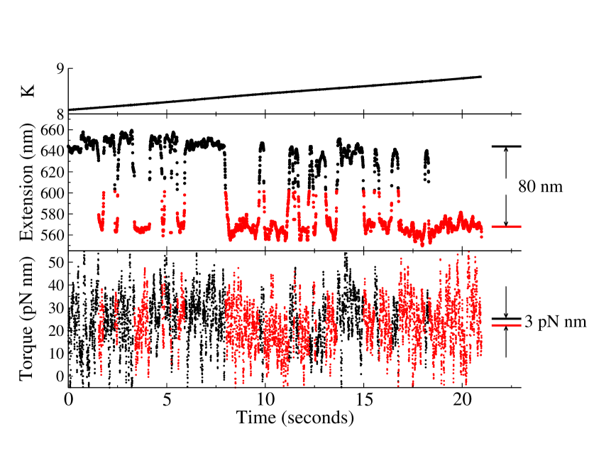
Figure 2: Directly measuring the torque jump by observing thermal hopping, for the same conditions as Fig. 1. As linking number $K$ is slowly increased near $K^{*}$, thermal fluctuations induce hopping between states with (CS) and without (SS) a plectoneme. Averaging over these two states gives a direct way of measuring the torque jump: analogously to a lock-in amplifier, we set a threshold in the extension signal to separately average the SS (black) and CS (red) data near the transition. Using multiple traces, we find an average torque jump of $\Delta\tau=2.9\pm 0.7$ pN nm for $L=2.2$ kbp at $F=2$ pN. Additionally, this value of $\Delta\tau$ implies (see text) that the transition should happen over a range of linking number $K$ (top) of about 0.9 turns, as it does.

The properties of stretched, unsupercoiled DNA are well-established. At small enough forces and torques that avoid both melting and supercoiling, DNA acts as a torsional spring with twist elastic constant $C$ Marko (2007): $\mathcal{F}_{\mathrm{SS}}(K,L)=\frac{C}{2}\left(2\pi\frac{K}{L}\right)^{2}L-F_{\mathrm{eff}}L$, where $K$ is the added linking number, $L$ is the overall (basepair) length of DNA, the effective force $F_{\mathrm{eff}}=F-kT\sqrt{F/B}$ Marko (2007) (see supplemental material), $F$ is the force applied to the ends of the DNA, $B=43\pm 3$ nm$\times kT$ is the DNA’s bending elastic constant, $C$ = $89\pm 3$ nm$\times kT$, and the thermal energy $kT=$ 4.09 pN nm for this experiment (at 23.5^∘C). Differentiating with respect to $K$ gives the torque: $\tau_{\mathrm{SS}}=\frac{1}{2\pi}\frac{d\mathcal{F}_{\mathrm{SS}}}{dK}=2\pi C\frac{K}{L}$. The extension of unsupercoiled DNA is shortened by thermal fluctuations, and in the relevant force regime is approximately given by $z_{\mathrm{SS}}=\xi(\tau_{\mathrm{SS}})L$, where Moroz and Nelson (1998)

$$\xi(\tau)=1-\frac{1}{2}\left[\frac{BF}{(kT)^{2}}-\left(\frac{\tau}{2kT}\right)^{2}-\frac{1}{32}\right]^{-1/2}.$$ (1)

Since supercoiling theories must include contact forces, they are less amenable to traditional theoretical methods. Even so, many theories have been successful in predicting properties of the CS; such methods have included detailed Monte Carlo simulations Vologodskii and Marko (1997), descriptions of the plectoneme as a simple helix Marko and Siggia (1995b); Neukirch (2004); Clauvelin et al. (2008), and a more phenomenological approach Marko (2007). However, none of these theories has yet been used to predict discontinuities at the SS–CS transition. Here we connect the free energy and extension predictions from any given model to the corresponding predictions for discontinuities at the transition.

We will use the framework of two-phase coexistence adopted by Marko Marko (2007, 2009) to describe the CS as consisting of two phases, each with constant free energy and extension per unit length of DNA . Since phase coexistence leads to a linear dependence on $K$ of the fraction of plectonemic DNA (keeping the torque fixed), in this model both $\mathcal{F}_{\mathrm{CS}}$ and $z_{\mathrm{CS}}$ are linear functions of added linking number $K$ and length $L$ (just as the free energy of an ice-water mixture is linear in the total energy, and the temperature remains fixed, as the ice melts). This linearity, along with the known properties of the SS, allows us to write $\mathcal{F}_{\mathrm{CS}}$ and $z_{\mathrm{CS}}$ as (see supplemental material)

$$\mathcal{F}_{\mathrm{CS}}(K,L) =\mathcal{F}_{0}+2\pi\tau K-\left(\frac{\tau^{2}}{2C}+F_{\mathrm{eff}}\right)L;$$ (2)

$$z_{\mathrm{CS}}(K,L) =-z_{0}-qK+\left(\xi(\tau)+\frac{\tau}{2\pi C}q\right)L,$$ (3)

where $q$ is the slope of extension versus linking number and $\tau$ is the CS torque. That is, $\mathcal{F}_{\mathrm{CS}}$ and $z_{\mathrm{CS}}$ are specified by four force-dependent values: their slopes with respect to $K$ ($\tau$ and $q$), which describe how the plectonemic phase coexists with the stretched phase; and $K=L=0$ offsets ($\mathcal{F}_{0}$ and $z_{0}$), which describe the extra free energy and extension necessary to form the interface between the phases — the end loop and tails of the plectoneme.

The experimental observables can then be written in terms of these four values. Easiest are $\tau$ and $q$, which are directly measured. Next, the linking number $K^{*}$ at the transition is found by equating the CS free energy with that of the SS: $\mathcal{F}_{\mathrm{CS}}(K^{*},L)=\mathcal{F}_{\mathrm{SS}}(K^{*},L)$ implies

$$K^{*}=\frac{L}{2\pi C}(\tau+\Delta\tau),\mathrm{with}~{}\Delta\tau=\sqrt{\frac{2C}{L}\mathcal{F}_{0}},$$ (4)

where $\Delta\tau$ is the jump in the torque at the transition. Lastly, inserting $K^{*}$ from Eq. (4) into Eq. (S12), we find the change in extension at the transition:

$$\Delta z =z_{0}+q\sqrt{\frac{L\mathcal{F}_{0}}{2\pi^{2}C}}-L\Big{(}\xi(\tau)-\xi(\tau+\sqrt{2C\mathcal{F}_{0}/L})\Big{)}.$$ (5)

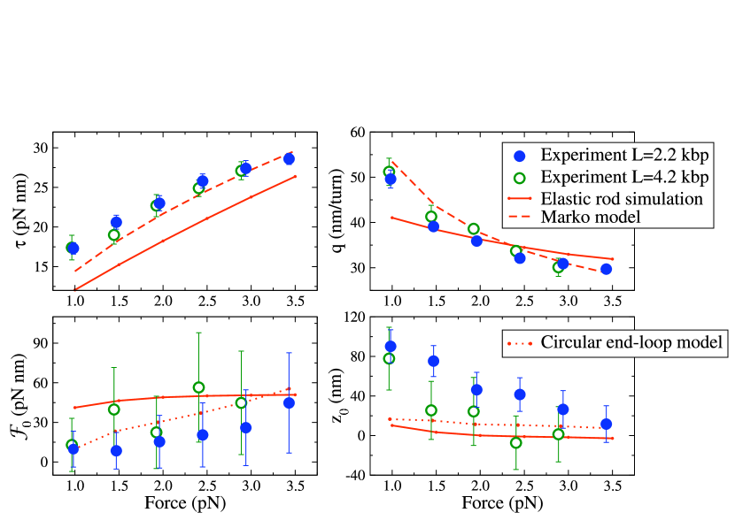
Figure 3: The four parameters describing the CS (coexisting torque $\tau$, extension versus linking number slope $q$, and the extra free energy $\mathcal{F}_{0}$ and extension $z_{0}$ necessary to form the end loop and tails of the plectoneme), as a function of applied force. The circles show values calculated from experimental data taken at two different overall DNA lengths $L$. Model predictions for our simulation endnote20 and Marko’s model Marko (2007) are shown as solid and dashed lines, respectively (using $S=0$ for $\mathcal{F}_{0}$ predictions). The circular end-loop model uses average $\tau$ and $q$ values from the experiment to predict $\mathcal{F}_{0}$ and $z_{0}$, shown as dotted lines.

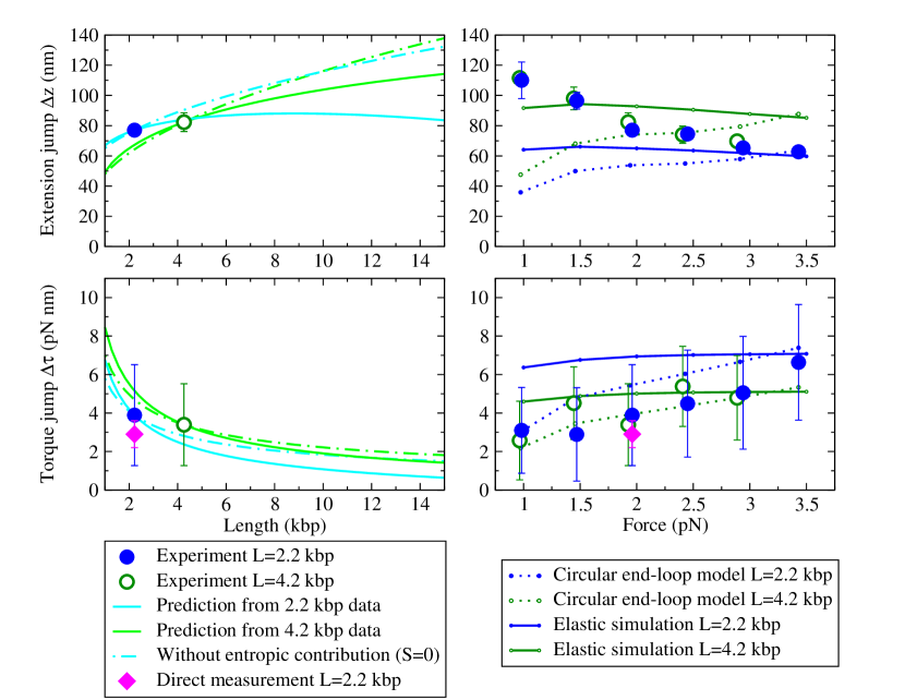
Figure 4: (Left) Predicted length-dependence of the extension and torque jumps at $F=2$ pN. Using the CS parameters extracted from the experiment at two different lengths, Eqs. (4) and (5) predict the $L$-dependence of $\Delta z$ and $\Delta\tau$. The circles show experimentally-measured values [with the torque jump here calculated from $K^{*}$ using Eq. (4)]. Without entropic corrections to $\mathcal{F}_{0}$ ($S=0$; dot-dashed lines) $\Delta z$ depends noticeably on $L$, but including an initial estimate of $S$ (solid lines) shows that entropic effects can significantly reduce this length-dependence. (Right) Force-dependence of the extension and torque jumps, and predictions from two models. Disagreements with experimental data can be understood in terms of the four CS parameters in Fig. 3. Also plotted as a diamond is $\Delta\tau$ measured using the direct method depicted in Fig. 2.

To additionally include entropic effects, we can write $\mathcal{F}_{0}=\mu-TS$, where $\mu$ is the energy cost for the end-loop and tails, and $S$ is the entropy coming from fluctuations in the location, length, and linking number of the plectoneme. Using an initial calculation of $S$ that includes these effects (in preparation; see supplemental material), we find that $S$ varies logarithmically with $L$, and that setting $S=0$ is a good approximation except when $L$ changes by large factors.

Given experimental data ($\tau$, $q$, $K^{*}$, and $\Delta z$), we can solve for the four CS parameters. The results from Ref. Forth et al. (2008) are shown as circles in Fig. 3 for the two overall DNA lengths tested. If we assume that the DNA is homogeneous, we expect the results to be independent of $L$ (except for a logarithmic entropic correction to $\mathcal{F}_{0}$ that would reduce it at the longer $L$ by about $kT\log 2\approx 5$ pN nm; see supplemental material). We do expect $\mathcal{F}_{0}$ and $z_{0}$ to be sensitive to the local properties of the DNA in the end-loop of the plectoneme, so we suspect that the difference in $z_{0}$ between the two measured lengths could be due to sequence dependence. With this data, we can also predict the length-dependence of the discontinuities, as shown in Fig. 4 (left). Here we included entropic corrections to $\mathcal{F}_{0}$ (see supplemental material), and we find that entropic effects significantly decrease the length-dependence of the extension jump.

Note that here we are solving for the experimental size of the torque jump using the observed $K^{*}$ and $\tau$ in Eq. (4). We also find direct evidence of $\Delta\tau$ in the data by averaging over the torque separately in the SS and CS near the transition (Fig. 2). With data taken at $F=2$ pN and $L=2.2$ kbp, we find $\Delta\tau=2.9\pm 0.7$ pN nm, in good agreement with the prediction from $K^{*}$ ($3.9\pm 2.6$ pN nm; see Fig. 4). We can also predict the width of the range of linking numbers around $K^{*}$ in which hopping between the two states is likely (where $|\Delta\mathcal{F}|<kT$): expanding to first order in $K-K^{*}$ gives a width of $2kT/(\pi\Delta\tau$). This predicts a transition region width of about 0.9 turns for the conditions in Fig. 2, agreeing well with the data.

We can now use various plectoneme models to calculate the four CS parameters, which in turn give predictions for the experimental observables. The results are shown as lines in Fig. 3 and Fig. 4 (right). As we expect entropic corrections to be small (changing $\mathcal{F}_{0}$ by at most about 5 pN nm), we set $S=0$ for these comparisons.

First, we test Marko’s phase coexistence model Marko (2007). The plectoneme is modeled as a phase with zero extension and an effective twist stiffness $P<C$. Shown as dashed lines in Fig. 3, the Marko model predicts the coexisting torque and extension slope well, with $P$ as the only fit parameter (we use $P=26$ nm). However, the Marko model (and any model that includes only terms in the free energy proportional to $L$) produces $\mathcal{F}_{0}=0$ and $z_{0}=0$.

In order to have a discontinuous transition, we must include the effects of the end loop and tails of the plectoneme. The simplest model assumes that the coexistence of stretched and plectonemic DNA requires one additional circular loop of DNA. Minimizing the total free energy for this circular end-loop model gives

$$\mathcal{F}_{0} =2\pi\sqrt{2BF_{\mathrm{eff}}}-2\pi\tau\mathrm{Wr}_{\mathrm{loop}};$$ (6)

$$z_{0} =2\pi\xi(\tau)\sqrt{B/(2F_{\mathrm{eff}})}-q\mathrm{Wr}_{\mathrm{loop}},$$ (7)

where $\mathrm{Wr}_{\mathrm{loop}}$ is the writhe taken up by the loop. For a perfect circle, $\mathrm{Wr}_{\mathrm{loop}}=1$, and $\mathrm{Wr}_{\mathrm{loop}}<1$ for a loop with two ends not at the same location. We chose $\mathrm{Wr}_{\mathrm{loop}}=0.8$ as a reasonable best fit to the data. Using the experimentally measured $\tau$ and $q$, the predictions are shown as solid lines in Fig. 3 and Fig. 4; $\mathcal{F}_{0}$ is fit fairly well, but $z_{0}$ is underestimated, especially at small applied forces.

In an attempt to more accurately model the shape of the plectoneme, we use an explicit simulation of an elastic rod, with elastic constants set to the known values for DNA. We must also include repulsion between nearby segments to keep the rod from passing through itself. Physically, this repulsion has two causes: screened Coulomb interaction of the charged strands and the loss of entropy due to limited fluctuations in the plectoneme. We use the repulsion free energy derived for the helical part of a plectoneme in Ref. Marko and Siggia (1995b), modified to a pairwise potential form (see supplemental material). We find that the simulation does form plectonemes (inset of Fig. 1), and we can extract the four CS parameters, shown as solid lines in Fig. 3 . Since $\mathcal{F}_{0}$ and $z_{0}$ are nonzero, we find discontinuities in the extension and torque at the transition; their magnitudes are plotted in Fig. 4.

Both the circular loop model and the simulation produce torque and extension jumps of the correct magnitude, but in both cases $\Delta z$ has an incorrect dependence on force and too much dependence on length. Our approach provides intuition about the causes of the discrepancies by singling out the four values (connected to different physical effects) that combine to produce the observed behavior. Specifically, we can better understand why the models’ predictions are length-dependent: as displayed in Fig. 4 (top left), the negligible length-dependence observed in experiment is caused by a subtle cancellation of a positive length-dependence [smaller than either model, and described by Eq. (5)] combined with a negative contribution coming from entropic effects. One would expect, then, that any plectoneme model (even one that explicitly includes entropic fluctuations) might easily miss this cancellation. In general, without this intuition, it is difficult to know where to start in improving the DNA models.

The largest uniform discrepancy happens at small applied forces, where both models underestimate $z_{0}$ , leading to an underestimate of $\Delta z$. We have examined various effects that could alter $z_{0}$, but none have caused better agreement (see also supplemental material). Adding to the circular end-loop model softening or kinking Du et al. (2008) at the plectoneme tip, or entropic terms from DNA cyclization theories Shimada and Yamakawa (1984); Odijk (1996), uniformly decreases $z_{0}$. Increasing $B$ in Eq. (6) by a factor of four (perhaps due to sequence dependence) does raise $z_{0}$ into the correct range, but it also raises $\mathcal{F}_{0}$ from Eq. (7) to values well outside the experimental ranges. Finally, $z_{0}$ would be increased if multiple plectonemes form at the transition, but we find that the measured values of $\mathcal{F}_{0}$ are too large to allow for more than one plectoneme in this experiment.

Support is acknowledged from NSF Grants DMR-0705167 and MCB-0820293, NIH Grant GM059849, and the Cornell Nanobiotechnology Center.

.1 Behavior of extended DNA with fluctuations

The behavior of extended DNA is appreciably affected by thermal fluctuations. For the applied forces in the range considered in this experiment, we can use the following fixed-torque free energy:

$$\frac{\mathcal{G}(\tau)}{L}=-F-\frac{\tau^{2}}{2C_{bare}}+\frac{kT}{B}\sqrt{BF-\frac{\tau^{2}}{4}},$$ (S1)

where the last term is the lowest-order correction due to fluctuations Moroz and Nelson (1998).

The fluctuations decrease the extension:

$$-\frac{\partial\mathcal{G}}{\partial F}=L\left[1-\frac{kT}{2}\left(BF-\frac{\tau^{2}}{4}\right)^{-1/2}\right].$$ (S2)

(The $-1/32$ in Eq. (1) comes from an approximation to a higher-order correction Moroz and Nelson (1998).)

Expanding the last term of Eq. (S1) to match the form of a “zero-temperature” chain, we can instead write

$$\frac{\mathcal{G}(\tau)}{L}=-F_{\mathrm{eff}}-\frac{\tau^{2}}{2C_{\mathrm{eff}}},$$ (S3)

where the effective force and twist elastic constant are given by

$$F_{\mathrm{eff}} =F-kT\sqrt{\frac{F}{B}}$$ (S4)

$$C_{\mathrm{eff}} =C_{bare}\left(1+kT\frac{C_{bare}}{4B\sqrt{BF}}\right)^{-1}.$$ (S5)

Note that $C_{\mathrm{eff}}$ is a function of force: there is less “softening” at higher forces. In the experiments of Forth et al., the renormalized $C_{\mathrm{eff}}$ was measured directly via the torque. However, the range of applied forces was small enough that $C_{\mathrm{eff}}$ did not change appreciably, and a single value of $C=(89~{}\mathrm{nm})kT$ was quoted. Here, we also use the same renormalized but force-independent value for $C$.

Changing Eq. (S3) to a fixed-linking-number expression via a Legendre transformation, we arrive at our expression for the straight state free energy (also found in Ref. Marko (2007)):

$$\mathcal{F}_{s}(K,L)=\frac{C}{2}\left(2\pi\frac{K}{L}\right)^{2}L-F_{\mathrm{eff}}L.$$ (S6)

.2 Derivation of linear expressions for $\mathcal{F}_{\mathrm{CS}}$ and $z_{\mathrm{CS}}$

We first write down the linear scaling of the free energy and extension with linking number. For any $\delta K$ that does not take the system out of the CS,

$$\mathcal{F}_{\mathrm{CS}}(K+\delta K,L) =\mathcal{F}_{\mathrm{CS}}(K,L)+2\pi\tau\delta K;$$ (S7)

$$z_{\mathrm{CS}}(K+\delta K,L) =z_{\mathrm{CS}}(K,L)-q\delta K,$$ (S8)

where $q$ is the slope of extension versus linking number and $\tau$ is the CS torque. Next, to find the scaling with increasing $L$, we imagine adding a piece of stretched DNA of length $\delta L$ at the coexisting torque (keeping the system in a stable CS). This also adds an amount of linking number that scales with $\delta L$, $\delta K[\delta L]=\tau\delta L/(2\pi C)$, which we will have to unwind to get back to the original $K$. First adding the piece of stretched DNA, and then unwinding to find the dependence on $L$ only, we find

$$\mathcal{F}_{\mathrm{CS}}(K,L+\delta L) =\mathcal{F}_{\mathrm{CS}}(K,L)-\left(\frac{\tau^{2}}{2C}+F_{\mathrm{eff}}\right)\delta L.$$ (S9)

Similarly for the extension, [using $\xi(\tau)$ from Eq. (1)]

$$z_{\mathrm{CS}}(K,L+\delta L) =z_{\mathrm{CS}}(K,L)+\left(\xi(\tau)+\frac{\tau}{2\pi C}q\right)\delta L.$$ (S10)

Combining Eqs. (S7) and (S8) with Eqs. (S9) and (S10), we can write the free energy and extension of the CS as linear in $K$ and $L$, each with a slope and an intercept:

$$\mathcal{F}_{\mathrm{CS}}(K,L) =\mathcal{F}_{0}+2\pi\tau K-\left(\frac{\tau^{2}}{2C}+F_{\mathrm{eff}}\right)L;$$ (S11)

$$z_{\mathrm{CS}}(K,L) =-z_{0}-qK+\left(\xi(\tau)+\frac{\tau}{2\pi C}q\right)L.$$ (S12)

Note that $C$ and $\xi(\tau)$ are known from experiments on stretched DNA, leaving the four anticipated force-dependent quantities to be described by a theory of supercoiling: $\tau$, $q$, $\mathcal{F}_{0}$, and $z_{0}$.

.3 Self-repulsion

It is essential to include a repulsive force between sections of the DNA that come near each other; without it, the rod can pass through itself, unphysically removing linking number in the process and preventing the formation of plectonemes. The physical origins of repulsive forces in DNA include both electrostatic and entropic effects. We use discretized versions of the repulsive interactions described in Ref. Marko and Siggia (1995b).

Electrostatic forces are modeled using a Debye-Huckel screened Coulomb interaction:

$$E_{\mathrm{SC}}(r)=\frac{|e_{-}\nu d|^{2}}{\epsilon}\frac{e^{-r/\lambda_{D}}}{r},$$ (S13)

where $\nu=8.4$ nm^-1 is the effective number of electron charges per unit length, $\lambda_{D}=0.8$ nm is the Debye screening length, and $e_{-}^{2}/\epsilon=2.9$ pN nm². (These values are dependent on the ionic concentration of the buffer, and were picked to match with $\approx 150$ mM NaCl.)

The entropic free energy of a helical structure is calculated in Ref. Marko and Siggia (1995b), coming from the increasing confinement of fluctuations in more tightly coiled structures. We use the same free energy, written as a pairwise interaction between segments:

$$E_{\mathrm{ent}}(r)=\frac{2^{5/3}\sqrt{\pi}\Gamma(1/3)}{\Gamma(5/6)}\frac{kTd^{2}}{(B/kT)^{1/3}r^{5/3}}.$$ (S14)

Since we also include straight parts of the DNA that should not have the same entropic interaction, we cut off the entropic potential at a distance of $2B/kT$, where the argument for the form of the potential breaks down Marko and Siggia (1995b).

.4 Extra terms in the circular end-loop model

Extra terms in the free energy that we have not considered would change the predictions of the circular end-loop model — these could include electrostatic interactions, entropic effects, etc. In fact, we can solve for the properties that such an extra free energy term (call it $\mathcal{F}_{\mathrm{extra}}$) would need to have in order to make the model match the experimental data.

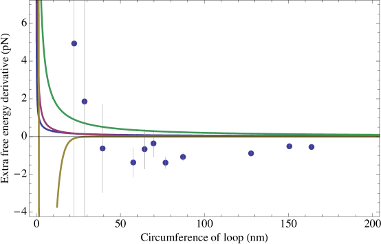
Figure S1: Entropic corrections from the literature do not help the circular end-loop model fit the data. The dots show the required free energy contribution $\mathcal{F}_{\mathrm{extra}}$ (top plot) and its derivative with respect to end-loop circumference $d\mathcal{F}_{\mathrm{extra}}/dL_{l}$ (bottom plot) that would produce an $\mathcal{F}_{0}$ and $z_{0}$ that match with the experiment (with $\mathrm{Wr}_{\mathrm{loop}}=0.8$). Bars on the top plot show the required derivative, the value of which is shown on the bottom plot. Vertical grey lines show one standard deviation error bars. Note especially the inability of any of the proposed entropic terms to match the well-constrained negative derivative at large end-loop circumferences (which happen at low force in the experiment); this produces $L_{l}$ (and thus $z_{0}$) that are too small at low forces. A lessening of the effective force felt by the end-loop of about 0.5 pN would help agreement, but none of the proposed corrections provides this.

Adding this unknown term, we have

$$\mathcal{F}_{l}(K_{l},L_{l})=\frac{C}{2L_{l}}\left[2\pi(K_{l}-\mathrm{Wr}_{\mathrm{loop}})\right]^{2}+(2\pi)^{2}\frac{B}{2L_{l}}+\mathcal{F}_{\mathrm{extra}}(K_{l},L_{l}).$$ (S15)

Since the terms we will imagine adding will not depend on $K_{l}$, we will assume that $\mathcal{F}_{\mathrm{extra}}$ is only a function of $L_{l}$. Setting the force and torque equal to the coexisting state values ($d\mathcal{F}_{l}/dL_{l}=-(F_{\mathrm{eff}}+\tau^{2}/(2C))$; $d\mathcal{F}_{l}/dK_{l}=2\pi\tau$) then gives

$$L_{l}^{*} =2\pi\sqrt{\frac{B}{2(F_{\mathrm{eff}}+d\mathcal{F}_{\mathrm{extra}}/dL_{l})}}$$ (S16)

$$K_{l}^{*} =\frac{\tau L_{l}^{*}}{2\pi C}+\mathrm{Wr}_{\mathrm{loop}}.$$ (S17)

We now use the fact that

$$\mathcal{F}_{0} =\mathcal{F}_{l}^{*}+(F_{\mathrm{eff}}+\frac{\tau^{2}}{2C})L_{l}^{*}-2\pi\tau K_{l}^{*}$$ (S18)

$$z_{0} =\xi(\tau)L_{l}^{*}-q\left(K_{l}^{*}-\frac{\tau L_{l}^{*}}{2\pi C}\right)$$ (S19)

to solve for the necessary values of $\mathcal{F}_{\mathrm{extra}}$ and $d\mathcal{F}_{\mathrm{extra}}/dL_{l}$ in order to match with the experimental $\mathcal{F}_{0}$ and $z_{0}$. We find

$$\mathcal{F}_{\mathrm{extra}} =\mathcal{F}_{0}+2\pi\tau\mathrm{Wr}_{\mathrm{loop}}-F_{\mathrm{eff}}L_{l}^{*}-\frac{2\pi^{2}B}{L_{l}^{*}}$$ (S20)

$$\frac{d\mathcal{F}_{\mathrm{extra}}}{dL_{l}} =\frac{2\pi^{2}B}{L_{l}^{*2}}-F_{\mathrm{eff}},$$ (S21)

where

$$L_{l}^{*}=\frac{z_{0}+q\mathrm{Wr}_{\mathrm{loop}}}{\xi(\tau)}.$$ (S22)

These required properties of the added free energy term are plotted in Fig. S1 for $\mathrm{Wr}_{\mathrm{loop}}=0.8$.

We can then test whether different possible extra free energy terms would match the requirements. Here we try four possibilities taken from the literature. First, there is electrostatic repulsion coming from like charges on opposite sides of the DNA circle. This looks like (using the Debye-Huckel formulation from Ref. Marko and Siggia (1995b))

$$\mathcal{F}_{\mathrm{extra}}^{\mathrm{electrostatic}}=kTl_{B}\nu^{2}K_{0}\left(\frac{L_{l}}{\pi\lambda_{D}}\right)L_{l}$$ (S23)

and is plotted in yellow in Fig. S1. Second, Odijk calculates the free energy for a circular DNA loop and finds terms in the free energy Odijk (1996) [Eq. (2.13)]

$$\mathcal{F}_{\mathrm{extra}}^{\mathrm{Odijk}}=kT\log{\frac{2\pi L}{B/(kT)}}-\frac{(kT)^{2}}{8B}L;$$ (S24)

this is plotted in purple in Fig. S1. Third, a similar term is found by Tkachenko in solving for the J-factor for unconstrained DNA cyclization [Eq. (4)]:

$$\mathcal{F}_{\mathrm{extra}}^{\mathrm{Tkachenko}}=5kT\log\frac{L}{B/(kT)};$$ (S25)

this is plotted in green in Fig. S1. Finally, we could imagine that entropic contributions from confinement similar to the one used by us for our elastic simulation could be important. Although the form was derived for a different configuration (superhelical DNA), we could try it to see if something similar might help. Integrating the confinement entropy from Marko and Siggia Marko and Siggia (1995b) over a circle gives

$$\mathcal{F}_{\mathrm{extra}}^{\mathrm{confinement}}=\frac{kT}{(B/kT)^{1/3}(L/(2\pi))^{2/3}}L,$$ (S26)

which is plotted in blue in Fig. S1.

Although these possible terms are only initial guesses at the possible corrections due to entropic and other effects, we see that they are all qualitatively unable to help, especially at long loop lengths, which is where the circular loop model fares worst at fitting the data.

.5 Calculating entropic contributions from fluctuations in plectoneme location, length, and linking number

To investigate entropic effects, we would like to find the free energy of states with multiple plectonemes , including fluctuations of linking number and length both within individual plectonemes and moving among different plectonemes. We can achieve this by calculating the partition function for a state with $n$ plectonemes, identifying unique states by the plectoneme positions $s_{i}$, the plectoneme lengths $L_{pi}$, and the plectoneme linking numbers $K_{pi}$:

$$Z_{n}(K,L)= \frac{1}{L_{0}^{n}}\int_{0}^{L}ds_{1}\int_{s_{1}}^{L}ds_{2}...\int_{s_{n-1}}^{L}ds_{n}$$ (S27)

$$\frac{1}{L_{0}^{n}}\int_{0}^{L}dL_{p1}\int_{0}^{L}dL_{p2}...\int_{0}^{L}dL_{pn}$$

$$\frac{1}{K_{0}^{n}}\int_{-\infty}^{\infty}dK_{p1}\int_{-\infty}^{\infty}dK_{p2}...\int_{-\infty}^{\infty}dL_{Kn}$$

$$\exp{\left[-\mathcal{F}_{n}(L,K,L_{pi},K_{pi})/kT\right]},$$

where we have neglected the complications coming from the possibility that plectonemes could overlap. The constants $L_{0}$ and $K_{0}$ set the length change and linking number change, respectively, that produce an independent state. Since we are only concerned with the free energy difference between the straight state and coexisting state, these constants would be set by the change in entropy of the degrees of freedom in the straight state that are lost to the collective modes we are integrating over in the coexisting state.

The first line of integrals represents the choice of where to put each plectoneme, which does not change the free energy ($\mathcal{F}_{n}$ does not depend on $s_{i}$). We therefore simply get a factor of $L^{n}$, divided by $n!$ since plectonemes are indistinguishable:

$$Z_{n}(K,L)=\frac{(L/L_{0})^{n}}{n!}\frac{1}{L_{0}^{n}K_{0}^{n}}\int_{0}^{L}\prod_{i}dL_{pi}\int_{-\infty}^{\infty}\prod_{i}dK_{pi}\exp{\big{[}-\mathcal{F}_{n}(L,K,\{L_{pi}\},\{K_{pi}\})/kT\big{]}}.$$ (S28)

Next we need to know the free energy of coexisting states that are away from the equilibrium plectoneme length and linking number. Assuming that the plectoneme free energy density is quadratic in linking number density (as in Marko’s model Marko (2007)), this turns out to be

$$\mathcal{F}_{n}(L,K,\{L_{pi}\},\{K_{pi}\})= \sum_{i=1}^{n}\frac{C}{2}\left(\frac{1}{1+v}\right)\left(2\pi\frac{K_{pi}}{L_{pi}}\right)^{2}L_{pi}$$ (S29)

$$+\frac{C}{2}\left(2\pi\frac{K-\sum K_{pi}}{L-\sum L_{pi}}\right)^{2}(L-\sum L_{pi})-F_{\mathrm{eff}}(L-\sum L_{pi})+n\mu,$$

where $\mu$ is the chemical potential for plectoneme ends and $v\equiv 2CF_{\mathrm{eff}}/\tau^{2}$.

We first evaluate the integrals over $K_{pi}$, which amount to $n$ Gaussian integrals; this gives

$$Z_{n}(K,L)=\frac{(L/L_{0})^{n}}{n!}\frac{1}{L_{0}^{n}K_{0}^{n}}\pi^{n/2}\int_{0}^{L} \prod_{i}dL_{pi}\left(\frac{\prod_{i}L_{pi}/c_{1}}{1+(1+v)\frac{\sum L_{pi}}{L-\sum L_{pi}}}\right)^{1/2}$$ (S30)

$$\exp{(-\frac{1}{kT}\left[\frac{\frac{C}{2}(2\pi K)^{2}}{L-\sum L_{pi}+(1+v)(\sum L_{pi})}-F_{\mathrm{eff}}(L-\sum L_{pi})+n\mu\right])}.$$

Now changing to unitless variables $x_{i}=L_{pi}/L_{p}$ and $y=L_{p}/L$, and rearranging to move all the factors that depend on the sum of the plectoneme lengths $y$ into the exponent, the term in the exponent becomes

$$f(y)=\frac{1}{kT}\left(\frac{\frac{C}{2}(2\pi K)^{2}/L}{1+vy}-F_{\mathrm{eff}}L(1-y)+n\mu\right)+\frac{1}{2}\log{\left(\frac{1+vy}{1-y}\right)},$$ (S31)

and we have

$$Z_{n}(K,L) =\frac{(L/L_{0})^{n}}{n!}\frac{1}{L_{0}^{n}K_{0}^{n}}\pi^{n/2}\int_{0}^{L}\prod_{i}dx_{i}\sqrt{\prod_{i}L_{pi}/c_{1}}\exp{[-f(\sum L_{pi}/L)]}$$ (S32)

$$=\frac{(L/L_{0})^{n}}{n!}\frac{1}{L_{0}^{n}K_{0}^{n}}\pi^{n/2}\int_{0}^{L}dL_{p}~{}\delta\left(\sum L_{pi}-L_{p}\right)\int_{0}^{L_{p}}\prod_{i}dL_{pi}\sqrt{\prod_{i}L_{pi}/c_{1}}\exp{[-f(L_{p}/L)]}$$

$$=\frac{(L/L_{0})^{n}}{n!}\frac{1}{L_{0}^{n}K_{0}^{n}}\pi^{n/2}\int_{0}^{L}dL_{p}\frac{L_{p}^{n}}{L_{p}}\left(\frac{L_{p}}{c_{1}}\right)^{n/2}\left[\int_{0}^{1}\prod_{i}dx_{i}\sqrt{\prod_{i}x_{i}}~{}\delta\left(\sum x_{i}-1\right)\right]\exp{[-f(L_{p}/L)]}$$

$$=\frac{(L/L_{0})^{2n}(L/c_{1})^{n/2}}{K_{0}^{n}}~{}\frac{\pi^{n/2}~{}\gamma_{n}}{n!}\int_{0}^{1}dy~{}\exp{[-(f(y)-\frac{3n-2}{2}\log y)]}.$$

The integral in large square brackets (characterizing fluctuations in the individual plectoneme lengths that do not change the total plectoneme length) gives a numerical constant $\gamma_{n}=\pi^{n/2}/(2^{n}\Gamma(3n/2))=2^{\lfloor\frac{n-1}{2}\rfloor}\pi^{\lfloor\frac{n}{2}\rfloor}/(3n-2)!!$. To evaluate the $y$ integral over total plectoneme length, we make a Gaussian approximation [noting that the total length is well-constrained by $f(y)$]. Then the fluctuations in the (fractional) total length of plectonemic DNA are of size

$$\sigma_{y}=\left(\frac{d^{2}}{dy^{2}}\left[f(y)-\frac{3n-2}{2}\log{y}\right]\Bigg{|}_{y^{*}}\right)^{-1/2},$$ (S33)

where $y^{*}$ is the equilibrium value of $y$, and the derivative is

$$\frac{d^{2}}{dy^{2}}\left[f(y)-\frac{3n-2}{2}\log{y}\right]=\frac{1}{2}\left(\frac{1}{(1-y)^{2}}+\frac{3n-2}{y^{2}}-\frac{v^{2}\left(1-\frac{8\pi^{2}CK^{2}}{LkT(1+vy)}\right)}{(1+vy)^{2}}\right).$$ (S34)

Without the entropic corrections, the equilibrium length is $y^{*}=(u-1)/v$, where $u=2\pi CK/(\tau L)$. We can safely use this value if we are far from $y^{*}=0$ and $y^{*}=1$, and get

$$\sigma_{y}=\frac{\sqrt{2}}{v}\left(\frac{1}{u}\frac{2\tau^{2}L}{kTC}-\frac{1}{u^{2}}+\frac{1}{(v-u+1)^{2}}+\frac{3n-2}{(u-1)^{2}}\right)^{-1/2}.$$ (S35)

[Since we are usually near $y^{*}=0$ at the transition, to calculate the length-dependence shown in Fig. 4 (left), we approximate $y^{*}$ numerically and use Eq. (S33) instead of Eq. (S35).] In the end, we have

$$Z_{n}(K,L)=\frac{(L/L_{0})^{2n}(L/c_{1})^{n/2}}{K_{0}^{n}}~{}\frac{\pi^{n/2}~{}\gamma_{n}}{n!}\sqrt{2\pi}\sigma_{y}\left(\frac{u-1}{v}\right)^{(3n-2)/2}\left(\frac{v-u+1}{uv}\right)^{1/2}\exp{[-\mathcal{F}(K,L)/kT]}.$$ (S36)

The full partition function for all plectonemic states is then

$$Z(K,L)=\sum_{n=1}^{\infty}Z_{n}(K,L)$$ (S37)

(which we can numerically approximate by truncating the series at a reasonable $n$), such that the coexisting state free energy is given by $\mathcal{F}_{\mathrm{CS}}(K,L)=-kT\log Z(K,L)$. For the experimental values, we find that only the single plectoneme $n=1$ state contributes significantly near the transition.

.6 Independence of results on entropic effects

In the paper, we have set the entropy from the previous section to zero ($S=0$) for most of the calculations. How would we expect that including $S$ would change any of the results?

First, $S$ would create a shift between the experimental $\mathcal{F}_{0}$ and the predictions from models that do not include fluctuations. We find that this shift is largely independent of force, and is mostly dependent on $L_{0}$. We do not currently have a way of calculating $L_{0}$, but we expect that it should be on the order of the persistence length of DNA, about 50 nm. We find that setting $L_{0}$ to about 100 nm makes the prefactor equal to 1, or equivalently sets $S=0$. If we assume that $L_{0}$ is about equal to the persistence length of DNA, we expect that we would need to shift the model predictions by at most about $kT\log 2\approx 5$ pN nm.

Second, we find that $S$ has a logarithmic dependence on $L$. This means that we expect $\mathcal{F}_{0}$ to decrease by something on the order of $kT\log(L_{2}/L_{1})$ when we increase the length from $L_{1}$ to $L_{2}$. For the experimental lengths (with $L_{2}\approx 2L_{1}$), this again corresponds to a shift of about 5 pN nm.

Shifting $\mathcal{F}_{0}$ by these amounts would slightly change only the theory curves for $\mathcal{F}_{0}$ (about 5 pN nm), $\Delta z$ (about 10 nm), and $\Delta\tau$ (about 1 pN nm).

References

- Strick et al. (1996) T. R. Strick, J.-F. Allemand, D. Bensimon, A. Bensimon, and V. Croquette, Science 271, 1835 (1996).
- Crut et al. (2007) A. Crut, D. A. Koster, R. Seidel, C. H. Wiggins, and N. H. Dekker, Proc. Natl. Acad. Sci. USA 104, 11957 (2007).
- van der Heijden et al. (2003) G. H. M. van der Heijden, S. Neukirch, V. G. A. Goss, and J. M. T. Thompson, Int. J. Mech. Sci. 45, 161 (2003).
- Forth et al. (2008) S. Forth, C. Deufel, M. Y. Sheinin, B. Daniels, J. P. Sethna, and M. D. Wang, Phys. Rev. Lett. 100, 148301 (2008).
- Marko and Siggia (1995a) J. F. Marko and E. D. Siggia, Macromolecules 28, 8759 (1995a).
- Marko (2007) J. F. Marko, Phys. Rev. E 76, 021926 (2007).
- Marko and Siggia (1995b) J. F. Marko and E. D. Siggia, Phys. Rev. E 52, 2912 (1995b).
- Neukirch (2004) S. Neukirch, Phys. Rev. Lett. 93, 198107 (2004).
- Fain et al. (1997) B. Fain, J. Rudnick, and S. Ostlund, Phys. Rev. E 55, 7364 (1997).
- Marko (2009) J. F. Marko, Proceedings of the Institute of Mathematics and its Applications , in press (2009).
- Moroz and Nelson (1998) J. D. Moroz and P. C. Nelson, Macromolecules 31, 6333 (1998).
- Vologodskii and Marko (1997) A. V. Vologodskii and J. F. Marko, Biophys. J. 73, 123 (1997).
- Clauvelin et al. (2008) N. Clauvelin, B. Audoly, and S. Neukirch, Macromolecules 41, 4479 (2008).
- Du et al. (2008) Q. Du, A. Kotlyar, and A. Vologodskii, Nucleic Acids Res. 36, 1120 (2008).
- Shimada and Yamakawa (1984) J. Shimada and H. Yamakawa, Macromolecules 17, 689 (1984).
- Odijk (1996) T. Odijk, J. Chem. Phys. 105, 1270 (1996).
- Moroz and Nelson (1997) J. D. Moroz and P. Nelson, Proc. Natl. Acad. Sci. USA 94, 14418 (1997).
Supplemental Material

References

- Strick et al. (1996) T. R. Strick, J.-F. Allemand, D. Bensimon, A. Bensimon, and V. Croquette, Science 271, 1835 (1996).
- Crut et al. (2007) A. Crut, D. A. Koster, R. Seidel, C. H. Wiggins, and N. H. Dekker, Proc. Natl. Acad. Sci. USA 104, 11957 (2007).
- van der Heijden et al. (2003) G. H. M. van der Heijden, S. Neukirch, V. G. A. Goss, and J. M. T. Thompson, Int. J. Mech. Sci. 45, 161 (2003).
- Forth et al. (2008) S. Forth, C. Deufel, M. Y. Sheinin, B. Daniels, J. P. Sethna, and M. D. Wang, Phys. Rev. Lett. 100, 148301 (2008).
- Marko and Siggia (1995a) J. F. Marko and E. D. Siggia, Macromolecules 28, 8759 (1995a).
- Marko (2007) J. F. Marko, Phys. Rev. E 76, 021926 (2007).
- Marko and Siggia (1995b) J. F. Marko and E. D. Siggia, Phys. Rev. E 52, 2912 (1995b).
- Neukirch (2004) S. Neukirch, Phys. Rev. Lett. 93, 198107 (2004).
- Fain et al. (1997) B. Fain, J. Rudnick, and S. Ostlund, Phys. Rev. E 55, 7364 (1997).
- Marko (2009) J. F. Marko, Proceedings of the Institute of Mathematics and its Applications , in press (2009).
- Moroz and Nelson (1998) J. D. Moroz and P. C. Nelson, Macromolecules 31, 6333 (1998).
- Vologodskii and Marko (1997) A. V. Vologodskii and J. F. Marko, Biophys. J. 73, 123 (1997).
- Clauvelin et al. (2008) N. Clauvelin, B. Audoly, and S. Neukirch, Macromolecules 41, 4479 (2008).
- Du et al. (2008) Q. Du, A. Kotlyar, and A. Vologodskii, Nucleic Acids Res. 36, 1120 (2008).
- Shimada and Yamakawa (1984) J. Shimada and H. Yamakawa, Macromolecules 17, 689 (1984).
- Odijk (1996) T. Odijk, J. Chem. Phys. 105, 1270 (1996).
- Moroz and Nelson (1997) J. D. Moroz and P. Nelson, Proc. Natl. Acad. Sci. USA 94, 14418 (1997).