Markov switching multinomial logit model: an application to accident injury severities

Abstract

In this study, two-state Markov switching multinomial logit models are proposed for statistical modeling of accident injury severities. These models assume Markov switching in time between two unobserved states of roadway safety. The states are distinct, in the sense that in different states accident severity outcomes are generated by separate multinomial logit processes. To demonstrate the applicability of the approach presented herein, two-state Markov switching multinomial logit models are estimated for severity outcomes of accidents occurring on Indiana roads over a four-year time interval. Bayesian inference methods and Markov Chain Monte Carlo (MCMC) simulations are used for model estimation. The estimated Markov switching models result in a superior statistical fit relative to the standard (single-state) multinomial logit models. It is found that the more frequent state of roadway safety is correlated with better weather conditions. The less frequent state is found to be correlated with adverse weather conditions.

,

1 Introduction

Vehicle accidents result in property damage, injuries and loss of people lives. Thus, research efforts in predicting accident severity are clearly very important. In the past there has been a large number of studies that focused on modeling accident severity outcomes. Common modeling approaches of accident severity include multinomial logit models, nested logit models, mixed logit models and ordered probit models (O’Donnell and Connor, 1996; Shankar and Mannering, 1996; Shankar et al., 1996; Duncan et al., 1998; Chang and Mannering, 1999; Carson and Mannering, 2001; Khattak, 2001; Khattak et al., 2002; Kockelman and Kweon, 2002; Lee and Mannering, 2002; Abdel-Aty, 2003; Kweon and Kockelman, 2003; Ulfarsson and Mannering, 2004; Yamamoto and Shankar, 2004; Khorashadi et al., 2005; Eluru and Bhat, 2007; Savolainen and Mannering, 2007; Milton et al., 2008). All these models involve nonlinear regression of the observed accident injury severity outcomes on various accident characteristics and related factors (such as roadway and driver characteristics, environmental factors, etc).

In our earlier paper, Malyshkina et al. (2008), which we will refer to as Paper I, we presented two-state Markov switching count data models of accident frequencies. In this study, which is a continuation of our work on Markov switching models, we present two-state Markov switching multinomial logit models for predicting accident severity outcomes. These models assume that there are two unobserved states of roadway safety, roadway entities (roadway segments) can switch between these states over time, and the switching process is Markovian. The two states intend to account for possible heterogeneity effects in roadway safety, which may be caused by various unpredictable, unidentified, unobservable risk factors that influence roadway safety. Because the risk factors can interact and change, roadway entities can switch between the two states over time. Two-state Markov switching multinomial logit models assume separate multinomial logit processes for accident severity data generation in the two states and, therefore, allow a researcher to study the heterogeneity effects in roadway safety.

2 Model specification

Markov switching models are parametric and can be fully specified by a likelihood function $f({\bf Y}|{\bf\Theta},{\cal M})$, which is the conditional probability distribution of the vector of all observations ${\bf Y}$, given the vector of all parameters ${\bf\Theta}$ of model ${\cal M}$. First, let us consider ${\bf Y}$. Let $N_{t}$ be the number of accidents observed during time period $t$, where $t=1,2,\ldots,T$ and $T$ is the total number of time periods. Let there be $I$ discrete outcomes observed for accident severity (for example, $I=3$ and these outcomes are fatality, injury and property damage only). Let us introduce accident severity outcome dummies $\delta^{(i)}_{t,n}$ that are equal to unity if the $i^{\rm th}$ severity outcome is observed in the $n^{\rm th}$ accident that occurs during time period $t$, and to zero otherwise. Here $i=1,2,\ldots,I$, $n=1,2,\ldots,N_{t}$ and $t=1,2,\ldots,T$. Then, our observations are the accident severity outcomes, and the vector of all observations ${\bf Y}=\{\delta^{(i)}_{t,n}\}$ includes all outcomes observed in all accidents that occur during all time periods. Second, let us consider model specification variable ${\cal M}$. It is ${\cal M}=\{M,{\bf X}_{t,n}\}$ and includes the model’s name $M$ (for example, $M=\mbox{``multinomial logit''}$) and the vector ${\bf X}_{t,n}$ of all accident characteristic variables (weather and environment conditions, vehicle and driver characteristics, roadway and pavement properties, and so on).

To define the likelihood function, we first introduce an unobserved (latent) state variable $s_{t}$, which determines the state of all roadway entities during time period $t$. At each $t$, the state variable $s_{t}$ can assume only two values: $s_{t}=0$ corresponds to one state and $s_{t}=1$ corresponds to the other state ($t=1,2,\ldots,T$). The state variable $s_{t}$ is assumed to follow a stationary two-state Markov chain process in time, which can be specified by time-independent transition probabilities as

$$P(s_{t+1}=1|s_{t}=0)=p_{0\rightarrow 1},\quad P(s_{t+1}=0|s_{t}=1)=p_{1\rightarrow 0}.$$ (1)

Here, for example, $P(s_{t+1}=1|s_{t}=0)$ is the conditional probability of $s_{t+1}=1$ at time $t+1$, given that $s_{t}=0$ at time $t$. Transition probabilities $p_{0\rightarrow 1}$ and $p_{1\rightarrow 0}$ are unknown parameters to be estimated from accident severity data. The stationary unconditional probabilities of states $s_{t}=0$ and $s_{t}=1$ are $\bar{p}_{0}=p_{1\rightarrow 0}/(p_{0\rightarrow 1}+p_{1\rightarrow 0})$ and $\bar{p}_{1}=p_{0\rightarrow 1}/(p_{0\rightarrow 1}+p_{1\rightarrow 0})$ respectively. Without loss of generality, we assume that (on average) state $s_{t}=0$ occurs more or equally frequently than state $s_{t}=1$. Therefore, $\bar{p}_{0}\geq\bar{p}_{1}$, and we obtain restriction

$$p_{0\rightarrow 1}\leq p_{1\rightarrow 0}.$$ (2)

We refer to states $s_{t}=0$ and $s_{t}=1$ as “more frequent” and “less frequent” states respectively.

Next, a two-state Markov switching multinomial logit (MSML) model assumes multinomial logit (ML) data-generating processes for accident severity in each of the two states. With this, the probability of the $i^{\rm th}$ severity outcome observed in the $n^{\rm th}$ accident during time period $t$ is

$$P_{t,n}^{(i)} = \left\{\begin{array}[]{ll}\displaystyle\frac{\exp({\mbox{\boldmath$\beta$}}_{(0),i}^{\prime}{\bf X}_{t,n})}{\sum_{j=1}^{I}\exp({\mbox{\boldmath$\beta$}}_{(0),j}^{\prime}{\bf X}_{t,n})}&\quad\mbox{if $s_{t}=0$},\\ \displaystyle\frac{\exp({\mbox{\boldmath$\beta$}}_{(1),i}^{\prime}{\bf X}_{t,n})\vphantom{\int\limits^{o}}}{\sum_{j=1}^{I}\exp({\mbox{\boldmath$\beta$}}_{(1),j}^{\prime}{\bf X}_{t,n})}&\quad\mbox{if $s_{t}=1$},\end{array}\right.$$ (5)

$$i = 1,2,\ldots,I,\quad n=1,2,\ldots,N_{t},\quad t=1,2,\ldots,T,\vphantom{\int}$$

Here prime means transpose (so ${\mbox{\boldmath$\beta$}}_{(0),i}^{\prime}$ is the transpose of ${\mbox{\boldmath$\beta$}}_{(0),i}$). Parameter vectors ${\mbox{\boldmath$\beta$}}_{(0),i}$ and ${\mbox{\boldmath$\beta$}}_{(1),i}$ are unknown estimable parameters of the two standard multinomial logit probability mass functions (Washington et al., 2003) in the two states, $s_{t}=0$ and $s_{t}=1$ respectively. We set the first component of ${\bf X}_{t,n}$ to unity, and, therefore, the first components of vectors ${\mbox{\boldmath$\beta$}}_{(0),i}$ and ${\mbox{\boldmath$\beta$}}_{(1),i}$ are the intercepts in the two states. In addition, without loss of generality, we set all $\beta$-parameters for the last severity outcome to zero, ${\mbox{\boldmath$\beta$}}_{(0),I}={\mbox{\boldmath$\beta$}}_{(1),I}={\bf 0}$.

If accident events are assumed to be independent, the likelihood function is

$$f({\bf Y}|{\bf\Theta},{\cal M})=\prod\limits_{t=1}^{T}\prod\limits_{n=1}^{N_{t}}\prod\limits_{i=1}^{I}\left[P_{t,n}^{(i)}\right]^{\delta^{(i)}_{t,n}}.$$ (6)

Here, because the state variables $s_{t,n}$ are unobservable, the vector of all estimable parameters ${\bf\Theta}$ must include all states, in addition to model parameters ($\beta$-s) and transition probabilities. Thus, ${\bf\Theta}=[{\mbox{\boldmath$\beta$}}_{(0)}^{\prime},{\mbox{\boldmath$\beta$}}_{(1)}^{\prime},p_{0\rightarrow 1},p_{1\rightarrow 0},{\bf S}^{\prime}]^{\prime}$, where vector ${\bf S}=[s_{1},s_{2},...,s_{T}]^{\prime}$ has length $T$ and contains all state values. Eqs. (1)-(6) define the two-state Markov switching multinomial logit (MSML) model considered here.

3 Model estimation methods

Statistical estimation of Markov switching models is complicated by unobservability of the state variables $s_{t}$. As a result, the traditional maximum likelihood estimation (MLE) procedure is of very limited use for Markov switching models. Instead, a Bayesian inference approach is used. Given a model ${\cal M}$ with likelihood function $f({\bf Y}|{\bf\Theta},{\cal M})$, the Bayes formula is

$$f({\bf\Theta}|{\bf Y},{\cal M})=\frac{f({\bf Y},{\bf\Theta}|{\cal M})}{f({\bf Y}|{\cal M})}=\frac{f({\bf Y}|{\bf\Theta},{\cal M})\pi({\bf\Theta}|{\cal M})}{\int f({\bf Y},{\bf\Theta}|{\cal M})\,d{\bf\Theta}}.$$ (7)

Here $f({\bf\Theta}|{\bf Y},{\cal M})$ is the posterior probability distribution of model parameters ${\bf\Theta}$ conditional on the observed data ${\bf Y}$ and model ${\cal M}$. Function $f({\bf Y},{\bf\Theta}|{\cal M})$ is the joint probability distribution of ${\bf Y}$ and ${\bf\Theta}$ given model ${\cal M}$. Function $f({\bf Y}|{\cal M})$ is the marginal likelihood function – the probability distribution of data ${\bf Y}$ given model ${\cal M}$. Function $\pi({\bf\Theta}|{\cal M})$ is the prior probability distribution of parameters that reflects prior knowledge about ${\bf\Theta}$. The intuition behind Eq. (7) is straightforward: given model ${\cal M}$, the posterior distribution accounts for both the observations ${\bf Y}$ and our prior knowledge of ${\bf\Theta}$.

In our study (and in most practical studies), the direct application of Eq. (7) is not feasible because the parameter vector ${\bf\Theta}$ contains too many components, making integration over ${\bf\Theta}$ in Eq. (7) extremely difficult. However, the posterior distribution $f({\bf\Theta}|{\bf Y},{\cal M})$ in Eq. (7) is known up to its normalization constant, $f({\bf\Theta}|{\bf Y},{\cal M})\propto f({\bf Y}|{\bf\Theta},{\cal M})\pi({\bf\Theta}|{\cal M})$. As a result, we use Markov Chain Monte Carlo (MCMC) simulations, which provide a convenient and practical computational methodology for sampling from a probability distribution known up to a constant (the posterior distribution in our case). Given a large enough posterior sample of parameter vector ${\bf\Theta}$, any posterior expectation and variance can be found and Bayesian inference can be readily applied. A reader interested in details is referred to our Paper I or to Malyshkina (2008), where we describe our choice of the prior distribution $\pi({\bf\Theta}|{\cal M})$ and the MCMC simulation algorithm. Although, in this study we estimate a two-state Markov switching multinomial logit model for accident severity outcomes and in Paper I we estimated a two-state Markov switching negative binomial model for accident frequencies, this difference is not essential for the Bayesian-MCMC model estimation methods. In fact, the main difference is in the likelihood function (multinomial logit as opposed to negative binomial). So we used the same our own numerical MCMC code, written in the MATLAB programming language, for model estimation in both studies. We tested our code on artificial data sets of accident severity outcomes. The test procedure included a generation of artificial data with a known model. Then these data were used to estimate the underlying model by means of our simulation code. With this procedure we found that the MSML models, used to generate the artificial data, were reproduced successfully with our estimation code.

For comparison of different models we use a formal Bayesian approach. Let there be two models ${\cal M}_{1}$ and ${\cal M}_{2}$ with parameter vectors ${\bf\Theta_{1}}$ and ${\bf\Theta_{2}}$ respectively. Assuming that we have equal preferences of these models, their prior probabilities are $\pi({\cal M}_{1})=\pi({\cal M}_{2})=1/2$. In this case, the ratio of the models’ posterior probabilities, $P({\cal M}_{1}|{\bf Y})$ and $P({\cal M}_{2}|{\bf Y})$, is equal to the Bayes factor. The later is defined as the ratio of the models’ marginal likelihoods (see Kass and Raftery, 1995). Thus, we have

$$\frac{P({\cal M}_{2}|{\bf Y})}{P({\cal M}_{1}|{\bf Y})}=\frac{f({\cal M}_{2},{\bf Y})/f(\bf Y)}{f({\cal M}_{1},{\bf Y})/f(\bf Y)}=\frac{f({\bf Y}|{\cal M}_{2})\pi({\cal M}_{2})}{f({\bf Y}|{\cal M}_{1})\pi({\cal M}_{1})}=\frac{f({\bf Y}|{\cal M}_{2})}{f({\bf Y}|{\cal M}_{1})},$$ (8)

where $f({\cal M}_{1},{\bf Y})$ and $f({\cal M}_{2},{\bf Y})$ are the joint distributions of the models and the data, $f({\bf Y})$ is the unconditional distribution of the data. As in Paper I, to calculate the marginal likelihoods $f({\bf Y}|{\cal M}_{1})$ and $f({\bf Y}|{\cal M}_{2})$, we use the harmonic mean formula $f({\bf Y}|{\cal M})^{-1}=E\left[\left.f({\bf Y}|{\bf\Theta},{\cal M})^{-1}\right|{\bf Y}\right]$, where $E(\ldots|{\bf Y})$ means posterior expectation calculated by using the posterior distribution. If the ratio in Eq. (8) is larger than one, then model ${\cal M}_{2}$ is favored, if the ratio is less than one, then model ${\cal M}_{1}$ is favored. An advantage of the use of Bayes factors is that it has an inherent penalty for including too many parameters in the model and guards against overfitting.

To evaluate the performance of model $\{{\cal M},{\bf\Theta}\}$ in fitting the observed data ${\bf Y}$, we carry out the Pearson’s $\chi^{2}$ goodness-of-fit test (Maher and Summersgill, 1996; Cowan, 1998; Wood, 2002; Press et al., 2007). We perform this test by Monte Carlo simulations to find the distribution of the Pearson’s $\chi^{2}$ quantity, which measures the discrepancy between the observations and the model predictions (Cowan, 1998). This distribution is then used to find the goodness-of-fit p-value, which is the probability that $\chi^{2}$ exceeds the observed value of $\chi^{2}$ under the hypothesis that the model is true (the observed value of $\chi^{2}$ is calculated by using the observed data ${\bf Y}$). For additional details, please see Malyshkina (2008).

4 Empirical results

The severity outcome of an accident is determined by the injury level sustained by the most injured individual (if any) involved into the accident. In this study we consider three accident severity outcomes: “fatality”, “injury” and “PDO (property damage only)”, which we number as $i=1,2,3$ respectively ($I=3$). We use data from 811720 accidents that were observed in Indiana in 2003-2006. As in Paper I, we use weekly time periods, $t=1,2,3,\ldots,T=208$ in total. Thus, the state $s_{t}$ can change every week. To increase the predictive power of our models, we consider accidents separately for each combination of accident type (1-vehicle and 2-vehicle) and roadway class (interstate highways, US routes, state routes, county roads, streets). We do not consider accidents with more than two vehicles involved. Thus, in total, there are ten roadway-class-accident-type combinations that we consider. For each roadway-class-accident-type combination the following three types of accident frequency models are estimated:

• First, we estimate a standard multinomial logit (ML) model without Markov switching by maximum likelihood estimation (MLE). We refer to this model as “ML-by-MLE”.

• Second, we estimate the same standard multinomial logit model by the Bayesian inference approach and the MCMC simulations. We refer to this model as “ML-by-MCMC”. As one expects, the estimated ML-by-MCMC model turned out to be very similar to the corresponding ML-by-MLE model (estimated for the same roadway-class-accident-type combination).

• Third, we estimate a two-state Markov switching multinomial logit (MSML) model by the Bayesian-MCMC methods. In order to make comparison of explanatory variable effects in different models straightforward, in the MSML model we use only those explanatory variables that enter the corresponding standard ML model. To obtain the final MSML model reported here, we also consecutively construct and use $60\%$, $85\%$ and $95\%$ Bayesian credible intervals for evaluation of the statistical significance of each $\beta$-parameter. As a result, in the final model some components of ${\mbox{\boldmath$\beta$}}_{(0)}$ and ${\mbox{\boldmath$\beta$}}_{(1)}$ are restricted to zero or restricted to be the same in the two states. We refer to this final model as “MSML”.

Note that the two states, and thus the MSML models, do not have to exist for every roadway-class-accident-type combination. For example, they will not exist if all estimated model parameters turn out to be statistically the same in the two states, ${\mbox{\boldmath$\beta$}}_{(0)}={\mbox{\boldmath$\beta$}}_{(1)}$, (which suggests the two states are identical and the MSML models reduce to the corresponding standard ML models). Also, the two states will not exist if all estimated state variables $s_{t}$ turn out to be close to zero, resulting in $p_{0\rightarrow 1}\ll p_{1\rightarrow 0}$ [compare to Eq. (2)], then the less frequent state $s_{t}=1$ is not realized and the process stays in state $s_{t}=0$.

Turning to the estimation results, the findings show that two states of roadway safety and the appropriate MSML models exist for severity outcomes of 1-vehicle accidents occurring on all roadway classes (interstate highways, US routes, state routes, county roads, streets), and for severity outcomes of 2-vehicle accidents occurring on streets. We did not find two states in the cases of 2-vehicle accidents on interstate highways, US routes, state routes and county roads (in these cases all estimated state variables $s_{t}$ were found to be close to zero). The model estimation results for severity outcomes of 1-vehicle accidents occurring on interstate highways, US routes and state routes are given in Tables 1–3. All continuous model parameters ($\beta$-s, $p_{0\rightarrow 1}$ and $p_{1\rightarrow 0}$) are given together with their $95\%$ confidence intervals (if MLE) or $95\%$ credible intervals (if Bayesian-MCMC), refer to the superscript and subscript numbers adjacent to parameter estimates in Tables 1–3. Table 4 gives summary statistics of all roadway accident characteristic variables ${\bf X}_{t,n}$ (except the intercept).

Table 1: Estimation results for multinomial logit models of severity outcomes of one-vehicle accidents on Indiana interstate highways

(the superscript and subscript numbers to the right of individual parameter estimates are $95\%$ confidence/credible intervals)

					MSML${}^{\,\rm c}$
${}^{{}^{\bf\displaystyle Variable}}$	${}^{{}^{\bf\displaystyle ML\mbox{\bf-}by\mbox{\bf-}MLE^{\,\rm a}}}$		${}^{{}^{\bf\displaystyle ML\mbox{\bf-}by\mbox{\bf-}MCMC^{\,\rm b}}}$		state $s=0$		state $s=1$
	fatality	injury	fatality	injury	fatality	injury	fatality	injury
Intercept (constant term)	$-11.9^{-10.1}_{-13.7}$	$-3.69^{-3.53}_{-3.84}$	$-12.4^{-10.6}_{-14.5}$	$-3.72^{-3.56}_{-3.88}$	$-12.2^{-10.5}_{-14.4}$	$-3.98^{-3.79}_{-4.17}$	$-12.2^{-10.5}_{-14.4}$	$-3.22^{-2.98}_{-3.45}$
Summer season (dummy)	$.235^{.329}_{.142}$	$.235^{.329}_{.142}$	$.237^{.329}_{.143}$	$.237^{.329}_{.143}$	$.176^{.293}_{.0551}$	$.176^{.293}_{.0551}$	$.176^{.293}_{.0551}$	$.615^{.959}_{.282}$
Thursday (dummy)	$-.798^{-.115}_{-1.48}$	–	$-.853^{-.206}_{-1.59}$	–	$-.872^{-.225}_{-1.61}$	–	$-.872^{-.225}_{-1.61}$	–
Construction at the accident location (dummy)	$-.418^{-.213}_{-.623}$	$-.418^{-.213}_{-.623}$	$-.425^{-.224}_{-.632}$	$-.425^{-.224}_{-.632}$	$-.566^{-.319}_{-.822}$	$-.566^{-.319}_{-.822}$	$-.566^{-.319}_{-.822}$	–
Daylight or street lights are lit up if dark (dummy)	$-.392^{-.0368}_{-.748}$	$.137^{.224}_{.0501}$	$-.387^{-.0301}_{-.740}$	$.143^{.230}_{.0568}$	$-.378^{-.0236}_{-.729}$	$.139^{.226}_{.0522}$	$-.378^{-.0236}_{-.729}$	$.139^{.226}_{.0522}$
Precipitation: rain/freezing rain/snow/sleet/hail (dummy)	$-1.38^{-.830}_{-1.92}$	$-.361^{-.264}_{-.457}$	$-1.41^{-.884}_{-1.99}$	$-.363^{-.267}_{-.460}$	$-1.54^{-1.03}_{-2.10}$	$-.563^{-.404}_{-.729}$	$-1.54^{-1.03}_{-2.10}$	–
Roadway surface is covered by snow/slush (dummy)	$-1.28^{-.0917}_{-2.46}$	$-.432^{-.280}_{-.583}$	$-1.43^{-.328}_{-2.84}$	$-.438^{-.288}_{-.590}$	$-.0515^{-.361}_{-.671}$	$-.0515^{-.361}_{-.671}$	$-.0515^{-.361}_{-.671}$	$-.0515^{-.361}_{-.671}$
Roadway median is drivable (dummy)	$.571^{.929}_{.213}$	–	$.577^{.939}_{.223}$	–	$.566^{.930}_{.211}$	–	$.566^{.930}_{.211}$	–
Roadway is at curve (dummy)	$.114^{.212}_{.0165}$	$.114^{.212}_{.0165}$	$.116^{.213}_{.0186}$	$.116^{.213}_{.0186}$	–	–	–	–
Primary cause of the accident is driver-related (dummy)	$4.24^{5.30}_{3.18}$	$1.53^{1.64}_{1.43}$	$4.39^{5.64}_{3.39}$	$1.54^{1.64}_{1.43}$	$4.48^{5.73}_{3.48}$	$2.00^{2.18}_{1.84}$	$4.48^{5.73}_{3.48}$	$.715^{.946}_{.468}$
Help arrived in 20 minutes or less after the crash (dummy)	$.790^{.887}_{.693}$	$.790^{.887}_{.693}$	$.790^{.891}_{.691}$	$.790^{.891}_{.691}$	$.785^{.886}_{.684}$	$.785^{.886}_{.684}$	$.785^{.886}_{.684}$	$.785^{.886}_{.684}$
The vehicle at fault is a motorcycle (dummy)	$3.88^{4.59}_{3.17}$	$2.74^{3.12}_{2.36}$	$3.87^{4.57}_{3.13}$	$2.75^{3.15}_{2.37}$	$4.61^{5.49}_{3.74}$	$3.23^{3.83}_{2.70}$	–	$1.39^{2.49}_{.326}$
Age of the vehicle at fault (in years)	$.0285^{.0370}_{.0201}$	$.0285^{.0370}_{.0201}$	$.0286^{.0370}_{.0201}$	$.0286^{.0370}_{.0201}$	–	$.0286^{.0371}_{.0200}$	–	$.0286^{.0371}_{.0200}$
Number of occupants in the vehicle at fault	$.366^{.463}_{.269}$	$.123^{.159}_{.0859}$	$.367^{.465}_{.264}$	$.123^{.159}_{.0861}$	$.366^{.464}_{.263}$	$.124^{.161}_{.0874}$	$.366^{.464}_{.263}$	$.124^{.161}_{.0874}$
Roadway traveled by the vehicle at fault is multi-lane and
divided two-way (dummy)	$2.60^{4.00}_{1.20}$	–	$2.86^{4.63}_{1.56}$	–	$2.86^{4.66}_{1.56}$	–	$2.86^{4.66}_{1.56}$	–
At least one of the vehicles involved was on fire (dummy)	$1.24^{2.12}$	$-.345^{-.0257}_{-.665}$	$1.18^{2.02}_{.206}$	$-.345^{-.0335}_{-.669}$	$1.66^{2.56}_{.621}$	$-.332^{-.0198}_{-.659}$	–	$-.332^{-.0198}_{-.659}$
Gender of the driver at fault (dummy)	–	$.328^{.410}_{.246}$	–	$.331^{.413}_{.248}$	–	$.224^{.338}_{.107}$	–	$.479^{.637}_{.328}$

Table 1: (Continued)

					MSML${}^{\,\rm c}$
${}^{{}^{\bf\displaystyle Variable}}$	${}^{{}^{\bf\displaystyle ML\mbox{\bf-}by\mbox{\bf-}MLE^{\,\rm a}}}$		${}^{{}^{\bf\displaystyle ML\mbox{\bf-}by\mbox{\bf-}MCMC^{\,\rm b}}}$		state $s=0$		state $s=1$
	fatality	injury	fatality	injury	fatality	injury	fatality	injury
Probability of severity outcome [$P_{t,n}^{(i)}$ given by Eq. (5)], averaged
over all values of explanatory variables ${\bf X}_{t,n}$	–	–	$.00724$	$.176$	$.00733$	$.174$	$.00672$	$.192$
Markov transition probability of jump $0\to 1$ ($p_{0\rightarrow 1}$)	–		–		$.151^{.254}_{.0704}$
Markov transition probability of jump $1\to 0$ ($p_{1\rightarrow 0}$)	–		–		$.330^{.532}_{.164}$
Unconditional probabilities of states 0 and 1 (${\bar{p}}_{0}$ and ${\bar{p}}_{1}$)	–		–		$.683^{.814}_{.540}$ and $.317^{.460}_{.186}$
Total number of free model parameters ($\beta$-s)	$25$		$25$		$28$
Posterior average of the log-likelihood (LL)	–		$-8486.78^{-8480.82}_{-8494.61}$		$-8396.78^{-8379.21}_{-8416.57}$
Max$(LL)$: estimated max. log-likelihood (LL) for MLE;
maximum observed value of LL for Bayesian-MCMC	$-8465.79\,{\rm(MLE)}\!$		$-8476.37\,{\rm(observed)}\!$		$-8358.97\,{\rm(observed)}\!$
Logarithm of marginal likelihood of data ($\ln[f({\bf Y}|{\cal M})]$)	–		$-8498.46^{-8494.22}_{-8499.21}$		$-8437.07^{-8424.77}_{-8440.02}$
Goodness-of-fit p-value	–		$0.255$		$0.222$
Maximum of the potential scale reduction factors (PSRF)${}^{\,\rm d}$	–		$1.00302$		$1.00060$
Multivariate potential scale reduction factor (MPSRF)${}^{\,\rm d}$	–		$1.00325$		$1.00067$
Number of available observations	accidents = fatalities + injuries + PDOs:   $19094=143+3369+15582$
a Standard (conventional) multinomial logit (ML) model estimated by maximum likelihood estimation (MLE).
b Standard multinomial logit (ML) model estimated by Markov Chain Monte Carlo (MCMC) simulations.
c Two-state Markov switching multinomial logit (MSML) model estimated by Markov Chain Monte Carlo (MCMC) simulations.
d PSRF/MPSRF are calculated separately/jointly for all continuous model parameters. PSRF and MPSRF are close to 1 for converged MCMC chains.

Table 2: Estimation results for multinomial logit models of severity outcomes of one-vehicle accidents on Indiana US routes

(the superscript and subscript numbers to the right of individual parameter estimates are $95\%$ confidence/credible intervals)

					MSML${}^{\,\rm c}$
${}^{{}^{\bf\displaystyle Variable}}$	${}^{{}^{\bf\displaystyle ML\mbox{\bf-}by\mbox{\bf-}MLE^{\,\rm a}}}$		${}^{{}^{\bf\displaystyle ML\mbox{\bf-}by\mbox{\bf-}MCMC^{\,\rm b}}}$		state $s=0$		state $s=1$
	fatality	injury	fatality	injury	fatality	injury	fatality	injury
Intercept (constant term)	$-6.51^{-5.00}_{-8.03}$	$-2.13^{-1.79}_{-2.47}$	$-6.62^{-5.16}_{-8.14}$	$-2.12^{-1.78}_{-2.47}$	$-5.72^{-4.69}_{-6.92}$	$-2.05^{-1.71}_{-2.40}$	$-5.72^{-4.69}_{-6.92}$	$-2.79^{-2.37}_{-3.23}$
Summer season (dummy)	$.514^{.894}_{.134}$	$.200^{.305}_{.0947}$	$.509^{.883}_{.124}$	$.200^{.305}_{.0951}$	$.190^{.300}_{.0789}$	$.190^{.300}_{.0789}$	$.190^{.300}_{.0789}$	–
Daylight or street lights are lit up if dark (dummy)	$-.498^{-.142}_{-.855}$	$.194^{.287}_{.101}$	$-.492^{-.136}_{-.848}$	$.203^{.296}_{.110}$	$-.493^{-.136}_{-.857}$	$.197^{.290}_{.105}$	–	$.197^{.290}_{.105}$
Snowing weather (dummy)	$-1.17^{-.170}_{-2.18}$	–	$-1.30^{-.357}_{-2.47}$	–	$-1.10^{-.151}_{-2.27}$	$.165^{.317}_{.0115}$	$-1.10^{-.151}_{-2.27}$	$.165^{.317}_{.0115}$
No roadway junction at the accident location (dummy)	$.701^{1.25}_{.149}$	$.217^{.335}_{.0994}$	$.727^{1.31}_{.199}$	$.213^{.331}_{.0968}$	$.787^{1.36}_{.259}$	$.214^{.332}_{.0965}$	$.787^{1.36}_{.259}$	$.214^{.332}_{.0965}$
Roadway is straight (dummy)	$-.741^{-.383}_{-1.10}$	$-.295^{-.191}_{-.399}$	$-.739^{-.377}_{-1.09}$	$-.296^{-.192}_{-.399}$	$-7.37^{-.372}_{-1.09}$	$-.294^{-.189}_{-.398}$	$-7.37^{-.372}_{-1.09}$	$-.294^{-.189}_{-.398}$
Primary cause of the accident is environment-related (dummy)	$-3.45^{-2.72}_{-4.18}$	$-1.89^{-1.78}_{-1.99}$	$-3.51^{-2.81}_{-4.32}$	$-1.89^{-1.79}_{-2.00}$	$-3.59^{-2.89}_{-4.40}$	$-2.09^{-1.96}_{-2.24}$	$-3.59^{-2.89}_{-4.40}$	$-.701^{-.263}_{-1.16}$
Help arrived in 10 minutes or less after the crash (dummy)	$.594^{.681}_{.507}$	$.594^{.681}_{.507}$	$.562^{.650}_{.475}$	$.562^{.650}_{.475}$	$.560^{.648}_{.472}$	$.560^{.648}_{.472}$	$.560^{.648}_{.472}$	$.560^{.648}_{.472}$
The vehicle at fault is a motorcycle (dummy)	$2.62^{3.47}_{1.78}$	$3.20^{3.55}_{2.86}$	$2.57^{3.38}_{1.65}$	$3.21^{3.56}_{2.87}$	$3.22^{3.58}_{2.88}$	$3.22^{3.58}_{2.88}$	$3.22^{3.58}_{2.88}$	$3.22^{3.58}_{2.88}$
Age of the vehicle at fault (in years)	$.0363^{.0444}_{.0283}$	$.0363^{.0444}_{.0283}$	$.0367^{.0448}_{.0287}$	$.0367^{.0448}_{.0287}$	–	$.0366^{.0447}_{.0285}$	–	$.0366^{.0447}_{.0285}$
Speed limit (used if known and the same for all vehicles involved)	$.0363^{.0631}_{.00950}$	$.0121^{.0178}_{.00640}$	$.0373^{.0643}_{.0117}$	$.0118^{.0176}_{.00616}$	$.0285^{.0495}_{.0104}$	$.0102^{.0178}_{.00635}$	–	$.0120^{.0178}_{.00635}$
Roadway traveled by the vehicle at fault is two-lane and
one-way (dummy)	$-.216^{.0417}_{-.391}$	$-.216^{.0417}_{-.391}$	$-.223^{.0517}_{-.398}$	$-.223^{.0517}_{-.398}$	$-.224^{.0504}_{-.401}$	$-.224^{.0504}_{-.401}$	$-.224^{.0504}_{-.401}$	$-.224^{.0504}_{-.401}$
At least one of the vehicles involved was on fire (dummy)	$1.19^{1.94}_{.439}$	–	$1.13^{1.85}_{.315}$	–	$1.27^{1.98}_{.452}$	–	$1.27^{1.98}_{.452}$	–
Age of the driver at fault (in years)	$.0114^{.0213}_{.00150}$	–	$.0113^{.0211}_{.00137}$	–	$.0101^{.0200}_{.0000542}$	–	–	–
Weekday (Monday through Friday) (dummy)	–	$-.104^{.0116}_{-.196}$	–	$-.104^{.0124}_{-.196}$	–	$-.125^{.0242}_{-.227}$	–	–
Gender of the driver at fault (dummy)	–	$.272^{.362}_{.183}$	–	$.276^{.365}_{.186}$	–	$.280^{.369}_{.190}$	–	$.280^{.369}_{.190}$

Table 2: (Continued)

					MSML${}^{\,\rm c}$
${}^{{}^{\bf\displaystyle Variable}}$	${}^{{}^{\bf\displaystyle ML\mbox{\bf-}by\mbox{\bf-}MLE^{\,\rm a}}}$		${}^{{}^{\bf\displaystyle ML\mbox{\bf-}by\mbox{\bf-}MCMC^{\,\rm b}}}$		state $s=0$		state $s=1$
	fatality	injury	fatality	injury	fatality	injury	fatality	injury
Probability of severity outcome [$P_{t,n}^{(i)}$ given by Eq. (5)], averaged
over all values of explanatory variables ${\bf X}_{t,n}$	–	–	$.00747$	$.179$	$.00823$	$.183$	$.00218$	$.158$
Markov transition probability of jump $0\to 1$ ($p_{0\rightarrow 1}$)	–		–		$.0767^{.157}_{.0269}$
Markov transition probability of jump $1\to 0$ ($p_{1\rightarrow 0}$)	–		–		$.613^{.864}_{.337}$
Unconditional probabilities of states 0 and 1 (${\bar{p}}_{0}$ and ${\bar{p}}_{1}$)	–		–		$.887^{.959}_{.770}$ and $.113^{.230}_{.0409}$
Total number of free model parameters ($\beta$-s)	$24$		$24$		$25$
Posterior average of the log-likelihood (LL)	–		$-7406.39^{-7400.61}_{-7414.03}$		$-7349.06^{-7335.46}_{-7364.47}$
Max$(LL)$: estimated max. log-likelihood (LL) for MLE;
maximum observed value of LL for Bayesian-MCMC	$-7384.05\,{\rm(MLE)}\!$		$-7396.37\,{\rm(observed)}\!$		$-7318.21\,{\rm(observed)}\!$
Logarithm of marginal likelihood of data ($\ln[f({\bf Y}|{\cal M})]$)	–		$-7417.98^{-7413.72}_{-7420.23}$		$-7377.49^{-7369.62}_{-7380.00}$
Goodness-of-fit p-value	–		$0.337$		$0.255$
Maximum of the potential scale reduction factors (PSRF)${}^{\,\rm d}$	–		$1.00319$		$1.00073$
Multivariate potential scale reduction factor (MPSRF)${}^{\,\rm d}$	–		$1.00376$		$1.00085$
Number of available observations	accidents = fatalities + injuries + PDOs:   $17797=138+3184+14485$
a Standard (conventional) multinomial logit (ML) model estimated by maximum likelihood estimation (MLE).
b Standard multinomial logit (ML) model estimated by Markov Chain Monte Carlo (MCMC) simulations.
c Two-state Markov switching multinomial logit (MSML) model estimated by Markov Chain Monte Carlo (MCMC) simulations.
d PSRF/MPSRF are calculated separately/jointly for all continuous model parameters. PSRF and MPSRF are close to 1 for converged MCMC chains.

Table 3: Estimation results for multinomial logit models of severity outcomes of one-vehicle accidents on Indiana state routes

(the superscript and subscript numbers to the right of individual parameter estimates are $95\%$ confidence/credible intervals)

					MSML${}^{\,\rm c}$
${}^{{}^{\bf\displaystyle Variable}}$	${}^{{}^{\bf\displaystyle ML\mbox{\bf-}by\mbox{\bf-}MLE^{\,\rm a}}}$		${}^{{}^{\bf\displaystyle ML\mbox{\bf-}by\mbox{\bf-}MCMC^{\,\rm b}}}$		state $s=0$		state $s=1$
	fatality	injury	fatality	injury	fatality	injury	fatality	injury
Intercept (constant term)	$-3.98^{-3.66}_{-4.30}$	$-1.67^{-1.53}_{-1.80}$	$-4.03^{-3.71}_{-4.36}$	$-1.71^{-1.58}_{-1.85}$	$-3.44^{-3.10}_{-3.79}$	$-1.68^{-1.54}_{-1.81}$	$-4.96^{-4.15}_{-5.96}$	$-1.68^{-1.54}_{-1.81}$
Summer season (dummy)	$.232^{.307}_{.156}$	$.232^{.307}_{.156}$	$.232^{.307}_{.157}$	$.232^{.307}_{.157}$	$.238^{.314}_{.163}$	$.238^{.314}_{.163}$	$.238^{.314}_{.163}$	$.238^{.314}_{.163}$
Roadway type (dummy: 1 if urban, 0 if rural)	$-.390^{-.302}_{-.478}$	$-.390^{-.302}_{-.478}$	$-.395^{-.306}_{-.483}$	$-.395^{-.306}_{-.483}$	–	$-.385^{-.296}_{-.474}$	$-2.05^{-.954}_{-3.62}$	$-3.85^{-.296}_{-.474}$
Daylight or street lights are lit up if dark (dummy)	$-.646^{-.408}_{-.884}$	$.193^{.261}_{.125}$	$-.641^{-.404}_{-.879}$	$.199^{.267}_{.132}$	$-.689^{-.448}_{-.931}$	–	$-.689^{-.448}_{-.931}$	$.277^{.378}_{.177}$
Precipitation: rain/freezing rain/snow/sleet/hail (dummy)	$-.854^{.466}_{-1.24}$	–	$-.868^{-.494}_{-1.27}$	–	$-.829^{-.448}_{-1.24}$	–	$-.829^{-.448}_{-1.24}$	–
Roadway median is drivable (dummy)	$-.583^{-.225}_{-.940}$	–	$-.596^{-.250}_{-.964}$	–	$-.589^{-.241}_{-.960}$	–	$-.589^{-.241}_{-.960}$	–
Roadway is straight (dummy)	$-.284^{-.214}_{-.353}$	$-.284^{-.214}_{-.353}$	$-.283^{-.214}_{-.352}$	$-.283^{-.214}_{-.352}$	$-.117^{-.0184}_{-.214}$	$-.117^{-.0184}_{-.214}$	$-.117^{-.0184}_{-.214}$	$-.465^{-.360}_{-.573}$
Primary cause of the accident is environment-related (dummy)	$-4.23^{-3.59}_{-4.86}$	$-1.83^{-1.76}_{-1.91}$	$-4.28^{-3.67}_{-4.97}$	$-1.84^{-1.76}_{-1.91}$	$-4.40^{-3.79}_{-5.10}$	$-2.30^{-2.16}_{-2.44}$	$-4.40^{-3.79}_{-5.10}$	$-1.41^{-1.26}_{-1.55}$
Help arrived in 20 minutes or less after the crash (dummy)	$.840^{.917}_{.762}$	$.840^{.917}_{.762}$	$.863^{.945}_{.781}$	$.863^{.945}_{.781}$	–	$.861^{.944}_{.778}$	$1.64^{2.64}_{.856}$	$.861^{.944}_{.778}$
The vehicle at fault is a motorcycle (dummy)	$3.10^{3.31}_{2.89}$	$3.10^{3.31}_{2.89}$	$3.10^{3.31}_{2.89}$	$3.10^{3.31}_{2.89}$	$3.37^{3.66}_{3.09}$	$3.37^{3.66}_{3.09}$	$3.37^{3.66}_{3.09}$	$2.82^{3.19}_{2.47}$
Number of occupants in the vehicle at fault	$.0557^{.0850}_{.0265}$	$.0557^{.0850}_{.0265}$	$.0565^{.0858}_{.0276}$	$.0565^{.0858}_{.0276}$	$.0942^{.138}_{.0528}$	$.0942^{.138}_{.0528}$	$.0942^{.138}_{.0528}$	–
At least one of the vehicles involved was on fire (dummy)	$1.90^{2.45}_{1.33}$	$.456^{.780}_{.133}$	$1.87^{2.42}_{1.28}$	$.447^{.768}_{.124}$	$1.87^{2.43}_{1.28}$	$.461^{.782}_{.137}$	$1.87^{2.43}_{1.28}$	$.461^{.782}_{.137}$
Age of the driver at fault (in years)	$\displaystyle{14.6^{21.4\vphantom{O^{o}}}_{7.80}}\atop\displaystyle{{}\times 10^{-3}}$	$\displaystyle{-2.80^{-.800\vphantom{O^{o}}}_{-4.70}}\atop\displaystyle{{}\times 10^{-3}}$	$\displaystyle{14.5^{21.3\vphantom{O^{o}}}_{7.67}}\atop\displaystyle{{}\times 10^{-3}}$	$\displaystyle{-2.71^{-.723\vphantom{O^{o}}}_{-4.69}}\atop\displaystyle{{}\times 10^{-3}}$	$\displaystyle{14.5^{21.4\vphantom{O^{o}}}_{7.63}}\atop\displaystyle{{}\times 10^{-3}}$	$\displaystyle{-2.46^{-.469\vphantom{O^{o}}}_{-4.44}}\atop\displaystyle{{}\times 10^{-3}}$	$\displaystyle{14.5^{21.4\vphantom{O^{o}}}_{7.63}}\atop\displaystyle{{}\times 10^{-3}}$	$\displaystyle{-2.46^{-.469\vphantom{O^{o}}}_{-4.44}}\atop\displaystyle{{}\times 10^{-3}}$
Gender of the driver at fault (dummy)	$-.496^{-.211}_{-.780}$	$.279^{.344}_{.214}$	$-.505^{-.225}_{-.794}$	$.278^{.343}_{.213}$	$-.473^{-.192}_{-.764}$	$.283^{.348}_{.218}$	$-.473^{-.192}_{-.764}$	$.283^{.348}_{.218}$
Age of the vehicle at fault (in years)	–	$.0334^{.0392}_{.0276}$	–	$.0335^{.0393}_{.0277}$	–	$.0332^{.0390}_{.0274}$	–	$.0332^{.0390}_{.0274}$
license state of the vehicle at fault is a U.S. state except Indiana
and its neighboring states (IL, KY, OH, MI)” indicator variable	–	$-.449^{-.217}_{-.681}$	–	$-.444^{-.217}_{-.679}$	–	$-.436^{-.208}_{-.671}$	–	$-.436^{-.208}_{-.671}$

Table 3: (Continued)

					MSML${}^{\,\rm c}$
${}^{{}^{\bf\displaystyle Variable}}$	${}^{{}^{\bf\displaystyle ML\mbox{\bf-}by\mbox{\bf-}MLE^{\,\rm a}}}$		${}^{{}^{\bf\displaystyle ML\mbox{\bf-}by\mbox{\bf-}MCMC^{\,\rm b}}}$		state $s=0$		state $s=1$
	fatality	injury	fatality	injury	fatality	injury	fatality	injury
Probability of severity outcome [$P_{t,n}^{(i)}$ given by Eq. (5)], averaged
over all values of explanatory variables ${\bf X}_{t,n}$	–	–	$.0089$	$.179$	$.00951$	$.180$	$.00804$	$.179$
Markov transition probability of jump $0\to 1$ ($p_{0\rightarrow 1}$)	–		–		$.335^{.465}_{.216}$
Markov transition probability of jump $1\to 0$ ($p_{1\rightarrow 0}$)	–		–		$.450^{.610}_{.313}$
Unconditional probabilities of states 0 and 1 (${\bar{p}}_{0}$ and ${\bar{p}}_{1}$)	–		–		$.574^{.681}_{.504}$ and $.426^{.496}_{.319}$
Total number of free model parameters ($\beta$-s)	$22$		$22$		$28$
Posterior average of the log-likelihood (LL)	–		$-13867.40^{-13861.92}_{-13874.73}$		$-13781.76^{-13765.02}_{-13800.89}$
Max$(LL)$: estimated max. log-likelihood (LL) for MLE;
maximum observed value of LL for Bayesian-MCMC	$-13846.60\,{\rm(MLE)}\!$		$-13858.00\,{\rm(observed)}\!$		$-13745.61\,{\rm(observed)}\!$
Logarithm of marginal likelihood of data ($\ln[f({\bf Y}|{\cal M})]$)	–		$-13877.89^{-13874.24}_{-13880.38}$		$-13820.20^{-13808.85}_{-13821.73}$
Goodness-of-fit p-value	–		$0.515$		$0.445$
Maximum of the potential scale reduction factors (PSRF)${}^{\,\rm d}$	–		$1.00027$		$1.00029$
Multivariate potential scale reduction factor (MPSRF)${}^{\,\rm d}$	–		$1.00041$		$1.00045$
Number of available observations	accidents = fatalities + injuries + PDOs:   $33528=302+6018+27208$
a Standard (conventional) multinomial logit (ML) model estimated by maximum likelihood estimation (MLE).
b Standard multinomial logit (ML) model estimated by Markov Chain Monte Carlo (MCMC) simulations.
c Two-state Markov switching multinomial logit (MSML) model estimated by Markov Chain Monte Carlo (MCMC) simulations.
d PSRF/MPSRF are calculated separately/jointly for all continuous model parameters. PSRF and MPSRF are close to 1 for converged MCMC chains.

Table 4: Summary statistics of roadway accident characteristic variables

Variable	Description
$\langle P_{t,n}^{(i)}\rangle_{X}$	probability of $i^{\rm th}$ severity outcome averaged over all values of explanatory variables ${\bf X}_{t,n}$
$p_{0\rightarrow 1}$	Markov transition probability of jump from state 0 to state 1 as time $t$ increases to $t+1$
$p_{1\rightarrow 0}$	Markov transition probability of jump from state 1 to state 0 as time $t$ increases to $t+1$
${\bar{p}}_{0}$ and ${\bar{p}}_{1}$	unconditional probabilities of states 0 and 1
$\#$ free par.	total number of free model coefficients ($\beta$-s)
averaged $LL\!$	posterior average of the log-likelihood (LL)
$\max(LL)$	for MLE it is the maximal value of $LL$ at convergence; for Bayesian-MCMC estimation
	it is the maximal observed value of LL during the MCMC simulations
marginal $LL\!$	logarithm of marginal likelihood of data, $\ln[f({\bf Y}|{\cal M})]$, given model ${\cal M}$
max(PSRF)	maximum of the potential scale reduction factors (PSRF) calculated separately for all
	continuous model parameters, PSRF is close to 1 for converged MCMC chains
MPSRF	multivariate PSRF calculated jointly for all parameters, close to 1 for converged MCMC
accept. rate	average rate of acceptance of candidate values during Metropolis-Hasting MCMC draws
$\#$ observ.	number of observations of accident severity outcomes available in the data sample
age0	”age of the driver at fault is $<18$ years” indicator variable (dummy)
age0o	”age of the oldest driver involved into the accident is $<18$ years” indicator variable
cons	”construction at the accident location” indicator variable
curve	”road is at curve” indicator variable
dark	”dark time with no street lights” indicator variable
darklamp	”dark AND street lights on” indicator variable
day	”daylight” indicator variable
dayt	”day hours: 9:00 to 17:00” indicator variable
driv	”road median is drivable” indicator variable
driver	”primary cause of the accident is driver-related” indicator variable
dry	”roadway surface is dry” indicator variable
env	”primary cause of the accident is environment-related” indicator variable
fog	”fog OR smoke OR smog” indicator variable
hl10	”help arrived in 10 minutes or less after the crash” indicator variable
hl20	”help arrived in 20 minutes or less after the crash” indicator variable
Ind	”license state of the vehicle at fault is Indiana” indicator variable
intercept	”constant term (intercept)” quantitative variable
jobend	”after work hours: from 16:00 to 19:00” indicator variable
light	”daylight OR street lights are lit up if dark” indicator variable
maxpass	”the largest number of occupants in all vehicles involved” quantitative variable
mm	”two male drivers are involved” indicator variable (used only if a 2-vehicle accident)
morn	”morning hours: 5:00 to 9:00” indicator variable
moto	”the vehicle at fault is a motorcycle” indicator variable

Table 4: (Continued)

Variable	Description
nigh	”late night hours: 1:00 to 5:00” indicator variable
nocons	”no construction at the accident location” indicator variable
nojun	”no road junction at the accident location” indicator variable
nonroad	”non-roadway crash (parking lot, etc.)” indicator variable
nosig	”no any traffic control device for the vehicle at fault” indicator variable
olddrv	”the driver at fault is older than the other driver” indicator var. (if a 2-vehicle accident)
oldvage	”age (in years) of the oldest vehicle involved” indicator variable
othUS	”license state of the vehicle at fault is a U.S. state except Indiana and its neighboring
	states (IL, KY, OH, MI)” indicator variable
precip	”precipitation: rain OR snow OR sleet OR hail OR freezing rain” indicator variable
priv	”road traveled by the vehicle at fault is a private drive” indicator variable
r21	”road traveled by the vehicle at fault is two-lane AND one-way” indicator variable
rmd2	”road traveled by the vehicle at fault is multi-lane AND divided two-way” indicator var.
singSUV	”one of the two vehicles involved is a pickup OR a van OR a sport utility vehicle”
	indicator variable (used only if a 2-vehicle accident)
singTR	”one of the two vehicles is a truck OR a tractor” indicator var. (if a 2-vehicle accident)
slush	”roadway surface is covered by snow/slush” indicator variable
snow	”snowing weather” indicator variable
str	”road is straight” indicator variable
sum	”summer season” indicator variable
sund	”Sunday” indicator variable
thday	”Thursday” indicator variable
vage	”age (in years) of the vehicle at fault” quantitative variable
veh	”primary cause of accident is vehicle-related” indicator variable
voldg	”the vehicle at fault is more than 7 years old” indicator variable
voldo	”age of the oldest vehicle involved is more than 7 years” indicator variable
wall	”road median is a wall” indicator variable
way4	”accident location is at a 4-way intersection” indicator variable
wint	”winter season” indicator variable
$X_{12}$	”road type” indicator variable (1 if urban, 0 if rural)
$X_{27}$	”number of occupants in the vehicle at fault” quantitative variable
$X_{29}$	”speed limit” quantitative var. (used if known and the same for all vehicles involved)
$X_{33}$	”at least one of the vehicles involved was on fire” indicator variable
$X_{34}$	”age (in years) of the driver at fault” quantitative variable
$X_{35}$	”gender of the driver at fault” indicator variable (1 if female, 0 if male)

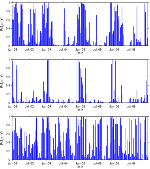
Figure 1: Weekly posterior probabilities $P(s_{t}=1|{\bf Y})$ for the MSML models estimated for severity of 1-vehicle accidents on interstate highways (top plot), US routes (middle plot) and state routes (bottom plot).

The top, middle and bottom plots in Figure 1 show weekly posterior probabilities $P(s_{t}=1|{\bf Y})$ of the less frequent state $s_{t}=1$ for the MSML models estimated for severity of 1-vehicle accidents occurring on interstate highways, US routes and state routes respectively. Because of space limitations, in this paper we do not report estimation results for severity of 1-vehicle accidents on county roads and streets, and for severity of 2-vehicle accidents. However, below we discuss our findings for all roadway-class-accident-type combinations. For unreported model estimation results see Malyshkina (2008).

We find that in all cases when the two states and Markov switching multinomial logit (MSML) models exist, these models are strongly favored by the empirical data over the corresponding standard multinomial logit (ML) models. Indeed, from lines “marginal $LL$” in Tables 1–3 we see that the MSML models provide considerable, ranging from $40.5$ to $61.4$, improvements of the logarithm of the marginal likelihood of the data as compared to the corresponding ML models. Thus, from Eq. (8) we find that, given the accident severity data, the posterior probabilities of the MSML models are larger than the probabilities of the corresponding ML models by factors ranging from $e^{40.5}$ to $e^{61.4}$. In the cases of 1-vehicle accidents on county roads, streets and the case of 2-vehicle accidents on streets, MSML models (not reported here) are also strongly favored by the empirical data over the corresponding ML models (Malyshkina, 2008).

Let us now consider the maximum likelihood estimation (MLE) of the standard ML models and an imaginary MLE estimation of the MSML models. We find that, in this imaginary case, a classical statistics approach for model comparison, based on the MLE, would also favors the MSML models over the standard ML models. For example, refer to line “max$(LL)$” in Table 1 given for the case of 1-vehicle accidents on interstate highways. The MLE gave the maximum log-likelihood value $-8465.79$ for the standard ML model. The maximum log-likelihood value observed during our MCMC simulations for the MSML model is equal to $-8358.97$. An imaginary MLE, at its convergence, would give a MSML log-likelihood value that would be even larger than this observed value. Therefore, if estimated by the MLE, the MSML model would provide large, at least $106.82$ improvement in the maximum log-likelihood value over the corresponding ML model. This improvement would come with only modest increase in the number of free continuous model parameters ($\beta$-s) that enter the likelihood function (refer to Table 1 under “# free par.”). Similar arguments hold for comparison of MSML and ML models estimated for other roadway-class-accident-type combinations (see Tables 2 and 3).

To evaluate the goodness-of-fit for a model, we use the posterior (or MLE) estimates of all continuous model parameters ($\beta$-s, $\alpha$, $p_{0\rightarrow 1}$, $p_{1\rightarrow 0}$) and generate $10^{4}$ artificial data sets under the hypothesis that the model is true. We find the distribution of $\chi^{2}$ and calculate the goodness-of-fit p-value for the observed value of $\chi^{2}$. For details, see Malyshkina (2008). The resulting p-values for our models are given in Tables 1–3. These p-values are around $00$–$100\%$. Therefore, all models fit the data well.

Now, refer to Table 5. The first six rows of this table list time-correlation coefficients between posterior probabilities $P(s_{t}=1|{\bf Y})$ for the six MSML models that exist and are estimated for six roadway-class-accident-type combinations (1-vehicle accidents on interstate highways, US routes, state routes, county roads, streets, and 2-vehicle accidents on streets). We see that the states for 1-vehicle accidents on all high-speed roads (interstate highways, US routes, state routes and county roads) are correlated with each other. The values of the corresponding correlation coefficients are positive and range from $0.263$ to $0.688$ (see Table 5). This result suggests an existence of common (unobservable) factors that can cause switching between states of roadway safety for 1-vehicle accidents on all high-speed roads.

Table 5: Correlations of the posterior probabilities $P(s_{t}=1|{\bf Y})$ with each other and with weather-condition variables (for the MSML model)

	1-vehicle,	1-vehicle,	1-vehicle,	1-vehicle,	1-vehicle,	2-vehicle,
	interstates	US routes	state routes	county roads	streets	streets
1-vehicle, interstates	$1$	$0.418$	$0.293$	$0.606$	$-0.013$	$-0.173$
1-vehicle, US routes	$0.418$	$1$	$0.263$	$0.688$	$-0.070$	$-0.155$
1-vehicle, state routes	$0.293$	$0.263$	$1$	$0.409$	$-0.047$	$-0.035$
1-vehicle, county roads	$0.606$	$0.688$	$0.409$	$1$	$-0.022$	$-0.051$
1-vehicle, streets	$-0.013$	$-0.070$	$-0.047$	$-0.022$	$1$	$0.115$
2-vehicle, streets	$-0.173$	$-0.155$	$-0.035$	$-0.051$	$0.115$	$1$
All year
Precipitation (inch)	$-0.139$	$-0.060$	$0.096$	$-0.037$	$0.067$	$0.146$
Temperature (${}^{o}F$)	$-0.606$	$-0.439$	$-0.234$	$-0.665$	$0.231$	$0.220$
Snowfall (inch)	$0.479$	$0.635$	$0.319$	$0.723$	$0.003$	$-0.100$
$\quad\quad\quad>0.0$ (dummy)	$0.695$	$0.412$	$0.382$	$0.695$	$-0.142$	$-0.131$
$\quad\quad\quad>0.1$ (dummy)	$0.532$	$0.585$	$0.328$	$0.847$	$-0.046$	$-0.161$
Wind gust (mph)	$0.108$	$0.100$	$0.087$	$0.206$	$0.164$	$0.051$
Fog / Frost (dummy)	$0.093$	$0.164$	$0.193$	$0.167$	$0.047$	$0.119$
Visibility distance (mile)	$-0.228$	$-0.221$	$-0.172$	$-0.298$	$-0.019$	$-0.081$
Winter (November - March)
Precipitation (inch)	$-0.134$	$-0.037$	$0.027$	$-0.053$	$0.065$	$0.356$
Temperature (${}^{o}F$)	$-0.595$	$-0.479$	$-0.397$	$-0.735$	$-0.008$	$0.236$
Snowfall (inch)	$0.439$	$0.592$	$0.375$	$0.645$	$0.157$	$-0.110$
$\quad\quad\quad>0.0$ (dummy)	$0.596$	$0.282$	$0.475$	$0.607$	$0.115$	$-0.142$
$\quad\quad\quad>0.1$ (dummy)	$0.445$	$0.518$	$0.370$	$0.789$	$0.112$	$-0.210$
Wind gust (mph)	$0.302$	$0.134$	$0.122$	$0.353$	$0.237$	$0.071$
Frost (dummy)	$0.537$	$0.544$	$0.440$	$0.716$	$0.052$	$-0.225$
Visibility distance (mile)	$-0.251$	$-.304$	$-0.249$	$-0.380$	$-0.155$	$-0.109$
Summer (May - September)
Precipitation (inch)	$0.000$	$0.006$	$0.259$	$0.096$	$0.047$	$-0.063$
Temperature (${}^{o}F$)	$0.179$	$0.149$	$0.113$	$0.037$	$0.062$	$0.155$
Snowfall (inch)	–	–	–	–	–	–
$\quad\quad\quad>0.0$ (dummy)	–	–	–	–	–	–
$\quad\quad\quad>0.1$ (dummy)	–	–	–	–	–	–
Wind gust (mph)	$-0.126$	$-.009$	$0.164$	$0.029$	$0.121$	$0.034$
Fog (dummy)	$0.203$	$0.193$	$0.275$	$0.101$	$-0.076$	$-0.011$
Visibility distance (mile)	$-0.139$	$-0.124$	$-0.062$	$-0.009$	$0.077$	$-0.094$

The remaining rows of Table 5 show correlation coefficients between posterior probabilities $P(s_{t}=1|{\bf Y})$ and weather-condition variables. These correlations were found by using daily and hourly historical weather data in Indiana, available at the Indiana State Climate Office at Purdue University (www.agry.purdue.edu/climate). For these correlations, the precipitation and snowfall amounts are daily amounts in inches averaged over the week and across Indiana weather observation stations. The temperature variable is the mean daily air temperature $(^{o}F)$ averaged over the week and across the weather stations. The wind gust variable is the maximal instantaneous wind speed (mph) measured during the 10-minute period just prior to the observational time. Wind gusts are measured every hour and averaged over the week and across the weather stations. The effect of fog/frost is captured by a dummy variable that is equal to one if and only if the difference between air and dewpoint temperatures does not exceed $5^{o}F$ (in this case frost can form if the dewpoint is below the freezing point $32^{o}F$, and fog can form otherwise). The fog/frost dummies are calculated for every hour and are averaged over the week and across the weather stations. Finally, visibility distance variable is the harmonic mean of hourly visibility distances, which are measured in miles every hour and are averaged over the week and across the weather stations.

From the results given in Table 5 we find that for 1-vehicle accidents on all high-speed roads (interstate highways, US routes, state routes and county roads), the less frequent state $s_{t}=1$ is positively correlated with extreme temperatures (low during winter and high during summer), rain precipitations and snowfalls, strong wind gusts, fogs and frosts, low visibility distances. It is reasonable to expect that roadway safety is different during bad weather as compared to better weather, resulting in the two-state nature of roadway safety.

The results of Table 5 suggest that Markov switching for road safety on streets is very different from switching on all other roadway classes. In particular, the states of roadway safety on streets exhibit low correlation with states on other roads. In addition, only streets exhibit Markov switching in the case of 2-vehicle accidents. Finally, states of roadway safety on streets show little correlation with weather conditions. A possible explanation of these differences is that streets are mostly located in urban areas and they have traffic moving at speeds lower that those on other roads.

Next, we consider the estimation results for the stationary unconditional probabilities $\bar{p}_{0}$ and $\bar{p}_{1}$ of states $s_{t}=0$ and $s_{t}=1$ for MSML models (see Section 2). In the cases of 1-vehicle accidents on interstate highways, US routes and state routes these transition probabilities are listed in lines “${\bar{p}}_{0}$ and ${\bar{p}}_{1}$” of Tables 1–3. In the cases of 1-vehicle accidents on county roads and 1- and 2-vehicle accidents on streets refer to Malyshkina (2008). We find that the ratio $\bar{p}_{1}/\bar{p}_{0}$ is approximately equal to $0.46$, $0.13$, $0.74$, $0.25$, $0.65$ and $0.36$ in the cases of 1-vehicle accidents on interstate highways, US routes, state routes, county roads, streets, and 2-vehicle accidents on streets respectively. Thus for some roadway-class-accident-type combinations (for example, 1-vehicle accidents on US routes) the less frequent state $s_{t}=1$ is quite rare, while for other combinations (for example, 1-vehicle accidents on state routes) state $s_{t}=1$ is only slightly less frequent than state $s_{t}=0$.

Finally, we set model parameters ($\beta$-s) to their posterior means, calculate the probabilities of fatality and injury outcomes by using Eq. (5) and average these probabilities over all values of the explanatory variables ${\bf X}_{t,n}$ observed in the data sample. We compare these probabilities across the two states of roadway safety, $s_{t}=0$ and $s_{t}=1$, for MSML models [refer to lines “$\langle P_{t,n}^{(i)}\rangle_{X}$” in Tables 1–3 and to Malyshkina (2008)]. We find that in many cases these averaged probabilities of fatality and injury outcomes do not differ very significantly across the two states of roadway safety (the only significant differences are for fatality probabilities in the cases of 1-vehicle accidents on US routes, county roads and streets). This means that in many cases states $s_{t}=0$ and $s_{t}=1$ are approximately equally dangerous as far as accident severity is concerned. We discuss this result in the next section.

5 Conclusions

In this study we found that two states of roadway safety and Markov switching multinomial logit (MSML) models exist for severity of 1-vehicle accidents occurring on high-speed roads (interstate highways, US routes, state routes, county roads), but not for 2-vehicle accidents on high-speed roads. One of possible explanations of this result is that 1- and 2-vehicle accidents may differ in their nature. For example, on one hand, severity of 1-vehicle accidents may frequently be determined by driver-related factors (speeding, falling a sleep, driving under the influence, etc). Drivers’ behavior might exhibit a two-state pattern. In particular, drivers might be overconfident and/or have difficulties in adjustments to bad weather conditions. On the other hand, severity of a 2-vehicle accident might crucially depend on the actual physics involved in the collision between the two cars (for example, head-on and side impacts are more dangerous than rear-end collisions). As far as slow-speed streets are concerned, in this case both 1- and 2-vehicle accidents exhibit two-state nature for their severity. Further studies are needed to understand these results. In this study, the important result is that in all cases when two states of roadway safety exist, the two-state MSML models provide much superior statistical fit for accident severity outcomes as compared to the standard ML models.

We found that in many cases states $s_{t}=0$ and $s_{t}=1$ are approximately equally dangerous as far as accident severity is concerned. This result holds despite the fact that state $s_{t}=1$ is correlated with adverse weather conditions. A likely and simple explanation of this finding is that during bad weather both number of serious accidents (fatalities and injuries) and number of minor accidents (PDOs) increase, so that their relative fraction stays approximately steady. In addition, most drivers are rational and they are likely take some precautions while driving during bad weather. From the results presented in Paper I we know that the total number of accidents significantly increases during adverse weather conditions. Thus, driver’s precautions are probably not sufficient to avoid increases in accident rates during bad weather.

References

- Abdel-Aty (2003) Abdel-Aty, M., 2003. Analysis of driver injury severity levels at multiple locations using ordered probit models. Journal of Safety Research 34(5), 597-603.
- Carson and Mannering (2001) Carson, J., Mannering, F.L., 2001. The effect of ice warning signs on ice-accident frequencies and severities. Accident Analysis and Prevention 33(1), 99-109.
- Chang and Mannering (1999) Chang, L.-Y., Mannering, F.L., 1999. Analysis of injury severity and vehicle occupancy in truck- and non-truck-involved accidents. Accident Analysis and Prevention 31(5), 579-592.
- Cowan (1998) Cowan, G., 1998. Statistical Data Analysis. Clarendon Press, Oxford Univ. Press, USA
- Duncan et al. (1998) Duncan, C., Khattak, A., Council, F., 1998. Applying the ordered probit model to injury severity in truck-passenger car rear-end collisions. Transportation Research Record 1635, 63-71.
- Eluru and Bhat (2007) Eluru, N., Bhat, C., 2007. A joint econometric analysis of seat belt use and crash-related injury severity. Accident Analysis and Prevention 39(5), 1037-1049.
- Kass and Raftery (1995) Kass, R.E., Raftery, A.E., 1995. Bayes Factors. Journal of the American Statistical Association 90(430), 773-795.
- Khattak (2001) Khattak, A., 2001. Injury severity in multi-vehicle rear-end crashes. Transportation Research Record 1746, 59-68.
- Khattak et al. (2002) Khattak, A., Pawlovich, D., Souleyrette, R., Hallmarkand, S., 2002. Factors related to more severe older driver traffic crash injuries. Journal of Transportation Engineering 128(3), 243-249.
- Khorashadi et al. (2005) Khorashadi, A., Niemeier, D., Shankar V., Mannering F.L., 2005. Differences in rural and urban driver-injury severities in accidents involving large trucks: an exploratory analysis. Accident Analysis and Prevention 37(5), 910-921.
- Kockelman and Kweon (2002) Kockelman, K., Kweon, Y.-J., 2002. Driver Injury Severity: An application of ordered probit models. Accident Analysis and Prevention 34(3), 313-321.
- Kweon and Kockelman (2003) Kweon, Y.-J., Kockelman, K., 2003. Overall injury risk to different drivers: combining exposure, frequency, and severity models. Accident Analysis and Prevention 35(4), 414-450.
- Lee and Mannering (2002) Lee, J., Mannering, F.L., 2002. Impact of roadside features on the frequency and severity of run-off-roadway accidents: an empirical analysis. Accident Analysis and Prevention 34(2), 149-161.
- Maher and Summersgill (1996) Maher M. J., Summersgill, I., 1996. A comprehensive methodology for the fitting of predictive accident models. Accid. Anal. Prev. 28(3), 281-296.
- Malyshkina (2006) Malyshkina, N.V., 2006. Influence of speed limit on roadway safety in Indiana. MS thesis, Purdue University. http://arxiv.org/abs/0803.3436
- Malyshkina (2008) Malyshkina, N. V., 2008. Markov switching models: an application of to roadway safety. PhD thesis, Purdue University. http://arxiv.org/abs/0808.1448
- Malyshkina et al. (2008) Malyshkina, N.V., Mannering, F.L., Tarko, A.P., 2008. Markov switching models: an application to Markov switching negative binomial models: an application to vehicle accident frequencies. Accepted for publication in Accident Analysis and Prevention. http://arxiv.org/abs/0811.1606
- Milton et al. (2008) Milton, J., Shankar, V., Mannering, F.L., 2008. Highway accident severities and the mixed logit model: an exploratory empirical analysis. Accident Analysis and Prevention 40(1), 260-266.
- O’Donnell and Connor (1996) O’Donnell, C., Connor, D., 1996. Predicting the severity of motor vehicle accident injuries using models of ordered multiple choice. Accident Analysis and Prevention 28(6), 739-753.
- Press et al. (2007) Press, W. H., Teukolsky, S. A., Vetterling, W. T., Flannery B. P., 2007. Numerical Recipes 3rd Edition: The Art of Scientific Computing. Cambridge Univ. Press, UK.
- Savolainen and Mannering (2007) Savolainen, P., Mannering, F.L., 2007. Probabilistic models of motorcyclists’ injury severities in single- and multi-vehicle crashes. Accident Analysis and Prevention 39(5), 955-963.
- Shankar and Mannering (1996) Shankar, V., Mannering, F.L., 1996. An exploratory multinomial logit analysis of single-vehicle motorcycle accident severity. Journal of Safety Research 27(3), 183-194.
- Shankar et al. (1996) Shankar, V., Mannering, F.L., Barfield, W., 1996. Statistical analysis of accident severity on rural freeways. Accident Analysis and Prevention 28(3), 391-401.
- Tsay (2002) Tsay, R. S., 2002. Analysis of financial time series: financial econometrics. John Wiley & Sons, Inc.
- Ulfarsson and Mannering (2004) Ulfarsson, G., Mannering, F.L., 2004. Differences in male and female injury severities in sport-utility vehicle, minivan, pickup and passenger car accidents. Accident Analysis and Prevention 36(2), 135-147.
- Washington et al. (2003) Washington, S.P., Karlaftis, M.G., Mannering, F.L., 2003. Statistical and econometric methods for transportation data analysis. Chapman & Hall/CRC.
- Wood (2002) Wood, G. R., 2002. Generalised linear accident models and goodness of fit testing. Accid. Anal. Prev. 34, 417-427.
- Yamamoto and Shankar (2004) Yamamoto, T., Shankar, V., 2004. Bivariate ordered-response probit model of driver’s and passenger’s injury severities in collisions with fixed objects. Accident Analysis and Prevention 36(5), 869-876.