Small-correlation expansions for the inverse Ising problem

Abstract

We present a systematic small-correlation expansion to solve the inverse Ising problem: find a set of couplings and fields corresponding to a given set of correlations and magnetizations. Couplings are calculated up to the third order in the correlations for generic magnetizations, and to the seventh order in the case of zero magnetizations; in addition we show how to sum some useful classes of diagrams exactly. The resulting expansion outperforms existing algorithms on the Sherrington-Kirkpatrick spin-glass model.

1 Introduction

Calculating average values of observables given a Hamiltonian is a general problem in statistical mechanics. This can done either analytically for a few exactly solvable systems or numerically through simulations with e.g. Monte Carlo techniques. These techniques give access, for not too low temperatures or too big systems, to the local magnetizations $m_{i}$ and spin-spin correlations $c_{ij}$ of an Ising sample, even in the notoriously complex case of spatially distributed interactions $J_{ij}$ and fields $h_{i}$ [1]. Much less attention has been brought in the physics literature to the inverse problem, that is, calculating the couplings and fields from the knowledge of the magnetizations and correlations, a problem known as Boltzmann-machine learning in statistical inference theory [2]. Yet the growing availability of data in many biological systems of interest as neural assemblies [3, 4], proteins [5], gene networks [6], … have strengthened the need for efficient techniques to infer interactions from correlations [7].

The purpose of this paper is to present a systematic expansion procedure to solve the inverse Ising problem. Given a set of observed magnetizations and correlations we look for the (a priori non uniform) couplings and fields of the Ising Hamiltonian reproducing those average observables at equilibrium. Our procedure is inspired from works by Plefka on mean-field spin glasses [10], and subsequent results by Georges and Yedidia [11, 12], who derived the free-energy of a spin-glass at fixed magnetization and interactions, performing a Legendre transform of the free-energy with respect to the fields. Technically speaking our work is an extension where one more Legendre transform, this time with respect to the interactions, is carried out to obtain the free-energy at fixed magnetization and correlations.

The need for calculating free-energies under some constraints is not new. One well-known example comes from the physics of gas or liquids, where one looks for the free-energy of interacting particles at fixed density and pair correlations [8]. Another example can be found in field theory, where one is interested in determining the thermodynamic potential for fixed average values of the field and two-point correlations [9]. Calculations generally rely on expansions in powers of the correlations around the non-interacting case which can be exactly handled. It is important to stress that, in contradistinction with the above-mentioned examples and most of the existing literature, our work deals with the case of discrete spin variables and non-translationally invariant interactions.

The plan of the paper is as follows. The general procedure for the expansion is exposed in Section 2. Section 3 is devoted to the generic case of non-zero magnetizations while Section 4 concentrates on the simpler case of zero magnetizations where the expansion can be pushed to higher orders. The results for the couplings are checked on two standard models: the unidimensional Ising model, and the Sherrington-Kirkpatrick (SK) model of a spin-glass. We show that our procedure for inferring couplings works better than existing methods for the SK model. The major technicalities are presented in the Appendices; the reader interested in explicit expressions for the couplings given the correlations and magnetizations can skip Section 2.

2 Procedure for the Small $c$ Expansion

We consider an Ising model over $N$ spins $\sigma_{i}=\pm 1$, $i=1,\ldots,N$, with Hamiltonian

$$H(\{S_{i}\})=-\sum_{i<j}J_{ij}\sigma_{i}\sigma_{j}-\sum_{i}h_{i}\sigma_{i}\ .$$ (1)

We want to find the values of couplings and the fields, $J^{*}_{ij},h^{*}_{i}$ such that the average values of the spins and of the spin-spin correlations match the prescribed magnetizations $m_{i}$ and connected correlations $c_{ij}$,

$$m_{i}=\frac{\partial\log Z}{\partial h_{i}}(\{J^{*}_{ij}\},\{h^{*}_{i}\})\quad,\qquad c_{ij}=\frac{\partial\log Z}{\partial J_{ij}}(\{J^{*}_{ij}\},\{h^{*}_{i}\})-m_{i}\;m_{j}$$ (2)

where the partition function (at unit temperature) reads

$$Z(\{J_{ij}\},\{h_{i}\})=\operatorname*{Tr}_{\{\sigma_{i}\}}e^{-H(\{\sigma_{i}\})}\ .$$ (3)

These couplings and fields are the ones that minimize the entropy of the Ising model at fixed magnetizations and correlations,

$$S(\{J_{ij}\},\{h_{i}\};\{m_{i}\},\{c_{ij}\}) = \log Z(\{J_{ij}\},\{h_{i}\})-\sum_{i<j}J_{ij}(c_{ij}+m_{i}m_{j})-\sum_{i}h_{i}m_{i}$$

$$= \log\operatorname*{Tr}_{\{\sigma_{i}\}}\exp\left\{\sum_{i<j}J_{ij}\left[(\sigma_{i}-m_{i})(\sigma_{j}-m_{j})-c_{ij}\right]+\sum_{i}\lambda_{i}(\sigma_{i}-m_{i})\right\}$$

where the new fields $\lambda_{i}$ are simply related to the physical fields $h_{i}$ through $\lambda_{i}=h_{i}+\sum_{j}J_{ij}m_{j}$.

The calculation of the entropy (2) for a given set of $J_{ij}$ and $\lambda_{i}$ is, in general, a computationally challenging task, not to say about its minimization. To obtain a tractable expression we multiply all (connected) correlations $c_{ij}$ in (2) by a small parameter $\beta$, which can be interpreted as a fictitious inverse temperature. The calculation of the entropy $S(\{J_{ij}\},\{\lambda_{i}\};\{m_{i}\},\{\beta\,c_{ij}\})$ is straightforward for $\beta=0$ since spins are uncoupled in this limit. The values of the couplings and fields minimizing the $\beta=0$ entropy are thus

$$J^{*}_{ij}(\beta=0)=0\quad,\qquad\lambda^{*}_{i}(\beta=0)=h^{*}_{i}(\beta=0)=\tanh^{-1}(m_{i})\ .$$ (5)

Our goal is to expand the couplings and fields in powers of $\beta$; to each order of the expansion the couplings and fields will be functions of the magnetizations and correlations. Ideally the couplings and fields we are looking for will be obtained when setting $\beta=1$ in the expansion.

To implement the expansion of $J_{ij}^{*}$ and $\lambda_{i}^{*}$ from equation (2) we proceed in the following way. First we define a potential $U$ over the spin configurations at inverse temperature $\beta$ through

$$U(\{\sigma_{i}\})=\sum_{i<j}J_{ij}^{*}(\beta)\left[(\sigma_{i}-m_{i})(\sigma_{j}-m_{j})-\beta\;c_{ij}\right]+\sum_{i}\lambda_{i}^{*}(\beta)(\sigma_{i}-m_{i})+\sum_{i<j}c_{ij}\int_{0}^{\beta}\mathrm{\;d}\beta^{\prime}J_{ij}^{*}(\beta^{\prime})$$ (6)

and a modified entropy, compare to (2),

$$\tilde{S}(\{m_{i}\},\{c_{ij}\},\beta)=\log\operatorname*{Tr}_{\{\sigma_{i}\}}e^{U(\{\sigma_{i}\})}\ .$$ (7)

Notice that $U$ depends on the coupling values $J^{*}_{ij}(\beta^{\prime})$ at all inverse temperatures $\beta^{\prime}<\beta$. The true entropy (at its minimum) and the modified entropy are simply related to each other,

$$S=\tilde{S}-\sum_{i<j}c_{ij}\int_{0}^{\beta}\mathrm{\;d}\beta^{\prime}J_{ij}^{*}(\beta^{\prime})\ .$$ (8)

The modified entropy $\tilde{S}$ (7) has an explicit dependence on $\beta$ through the potential $U$ (6), and an implicit dependence through the couplings and the fields. As the latter are chosen to minimize $S$ the full derivative of $\tilde{S}$ with respect to $\beta$ coincides with its partial derivative, and we get

$$\frac{d\tilde{S}}{d\beta}=-\sum_{i<j}c_{ij}\;J_{ij}^{*}(\beta)+\sum_{i<j}c_{ij}\;J_{ij}^{*}(\beta)=0\ .$$ (9)

The above equality is true for any $\beta$. Consequently $\tilde{S}$ is constant, and equal to its $\beta=0$ value, that is, to the entropy of $N$ uncoupled spins with known magnetizations $\{m_{i}\}$.

We now present three facts, shown in the Appendices:

• For any integer $k\geq 2$,

  $$\left.\frac{\partial^{k}\tilde{S}}{\partial\beta^{k}}\right|_{0}=-\sum_{i<j}c_{ij}\left.\frac{\partial^{k-1}J_{ij}^{*}}{\partial\beta^{k-1}}\right|_{0}+Q_{k}$$ (10)

  where $Q_{k}$ is a (known) function of the magnetizations, correlations, and of the derivatives in $\beta=0$ of the couplings $J_{ij}^{*}$ and fields $\lambda_{i}^{*}$ of order $\leq\max(1,k-2)$. See Appendices A and C. Recall that $\tilde{S}$ is constant by virtue of (9) thus both sides of (10) vanishes.

• For any integer $k\geq 2$ the $k^{th}$ derivative of $\lambda^{*}_{i}$ in $\beta=0$ can be calculated from the magnetizations and the knowledge of the derivatives in $\beta=0$ of the couplings $J_{ij}^{*}$ of order $\leq k-1$. See Appendix B.

• The first derivative of the couplings in $\beta=0$ is given by

  $$\left.\frac{\partial J_{ij}^{*}}{\partial\beta}\right|_{0}=\frac{c_{ij}}{(1-m_{i}^{2})(1-m_{j}^{2})}\ .$$ (11)

  See Appendix A.1.

Those facts allow us to calculate the derivatives of the couplings in $\beta=0$ to any order in a recursive way. Let $k\geq 3$. From the definition (2) of the entropy

$$\frac{\partial S}{\partial c_{ij}}(\{J^{*}_{ij}\},\{\lambda^{*}_{i}\};\{m_{i}\},\{\beta\;c_{ij}\})=-\beta\;J_{ij}^{*}\ .$$ (12)

Differentiation of the above equation $k$ times with respect to $\beta$ in $\beta=0$ gives

$$\left.\frac{\partial^{k}}{\partial\beta^{k}}\right|_{0}\frac{\partial S}{\partial c_{ij}}(\{J^{*}_{ij}\},\{\lambda^{*}_{i}\};\{m_{i}\},\{\beta\;c_{ij}\})=-k\;\left.\frac{\partial^{k-1}J_{ij}^{*}}{\partial\beta^{k-1}}\right|_{0}\ .$$ (13)

Using relationship (8) we obtain

$$\frac{\partial}{\partial c_{ij}}\left[\left.\frac{\partial^{k}\tilde{S}}{\partial\beta^{k}}\right|_{0}-\sum_{r<s}c_{rs}\,\left.\frac{\partial^{k-1}\tilde{J}_{rs}^{*}}{\partial\beta^{k-1}}\right|_{0}\right]=-k\;\left.\frac{\partial^{k-1}J_{ij}^{*}}{\partial\beta^{k-1}}\right|_{0}\ .$$ (14)

We now use that $\tilde{S}$ is constant and fact A to deduce

$$\left.\frac{\partial^{k-1}J_{ij}^{*}}{\partial\beta^{k-1}}\right|_{0}=\frac{1}{k}\;\frac{\partial Q_{k}}{\partial c_{ij}}\ .$$ (15)

As a consequence the $(k-1)^{th}$ derivative of $J_{ij}^{*}$ in $\beta=0$ is a known function of the derivatives in $\beta=0$ of the couplings $J_{ij}^{*}$ and fields $\lambda_{i}^{*}$ of order $\leq k-2$ (and of the magnetizations and correlations). Using fact B we express all the derivatives of the fields in terms of the derivatives of the couplings of order $\leq k-2$. Hence we can compute the $(k-1)^{th}$ derivative of the couplings from the knowledge of all derivatives with lower orders. The recursive procedure uses fact C as a starting point to generate all derivatives.

3 General results for non-zero magnetizations

3.1 Explicit expansions of the entropy, couplings and fields

The procedure exposed in the previous Section has allowed us to expand the entropy $S$ and the fields $h_{i}$ up to order $c^{4}$ and the couplings up to order $c^{3}$. Details are given in Appendix A. We define

$$L_{i}=1-m_{i}^{2}\quad,\qquad K_{ij}=\frac{c_{ij}}{L_{i}L_{j}}\ .$$ (16)

The entropy reads

$$S = -\sum_{i}\left[\frac{1+m_{i}}{2}\ln\frac{1+m_{i}}{2}+\frac{1-m_{i}}{2}\ln\frac{1-m_{i}}{2}\right]$$ (17)

$$- \frac{\beta^{2}}{2}\sum_{i<j}K_{ij}^{2}L_{i}L_{j}+\frac{2}{3}\beta^{3}\sum_{i<j}K_{ij}^{3}m_{i}m_{j}L_{i}L_{j}+\beta^{3}\sum_{i<j<k}K_{ij}K_{jk}K_{ki}L_{i}L_{j}L_{k}$$

$$- \frac{\beta^{4}}{12}\sum_{i<j}K_{ij}^{4}\left[1+3m_{i}^{2}+3m_{j}^{2}+9m_{i}^{2}m_{j}^{2}\right]L_{i}L_{j}-\frac{\beta^{4}}{2}\sum_{i<j}\sum_{k}K_{ik}^{2}K_{kj}^{2}L_{k}^{2}L_{i}L_{j}$$

$$- \beta^{4}\sum_{i<j<k<l}(K_{ij}K_{jk}K_{kl}K_{li}+K_{ik}K_{kj}K_{lj}K_{il}+K_{ij}K_{jl}K_{lk}K_{ki})L_{i}L_{j}L_{k}L_{l}$$

$$+ O(\beta^{5})$$

The terms in the expansion can be represented diagrammatically. A point in a diagram represents a spin, and a line represents a $K_{ij}$ link. We do not represent the polynomial in the variables $\{m_{i}\}$ that multiplies each diagram. Summation over the indices is implicit.

$$S(\{c_{kl}\},\{m_{i}\},\beta) = -\begin{tabular}[]{c}\includegraphics[scale={.4}]{spin.epsi}\end{tabular}-\frac{1}{2}\begin{tabular}[]{c}\includegraphics[scale={.4}]{loop1.epsi}\end{tabular}+\frac{2}{3}\begin{tabular}[]{c}\includegraphics[scale={.4}]{2spins_3.epsi}\end{tabular}+\begin{tabular}[]{c}\includegraphics[scale={.4}]{loop2.epsi}\end{tabular}$$ (22)

$$- \frac{1}{12}\begin{tabular}[]{c}\includegraphics[scale={.4}]{loop_d1.epsi}\end{tabular}-\frac{1}{2}\begin{tabular}[]{c}\includegraphics[scale={.4}]{3spins_lin.epsi}\end{tabular}-\begin{tabular}[]{c}\includegraphics[scale={.4}]{loop3.epsi}\end{tabular}$$ (26)

In contradistinction with [11] the expansion includes non-irreducible diagrams. It should be noted that, as in [11], the Feynman rules of these graphs is unknown even in the $m_{i}=0$ case, which makes impossible to do the expansion by a simple enumeration of the diagrams. The result for $J_{ij}$ is

$$J_{ij}^{*}(\{c_{kl}\},\{m_{i}\},\beta) = \beta K_{ij}-2\beta^{2}m_{i}m_{j}K_{ij}^{2}-\beta^{2}\sum_{k}K_{jk}K_{ki}L_{k}$$ (27)

$$+ \frac{1}{3}\beta^{3}K_{ij}^{3}\left[1+3m_{i}^{2}+3m_{j}^{2}+9m_{i}^{2}m_{j}^{2}\right]+\beta^{3}\sum_{\begin{subarray}{c}k\\ (\neq i,\,\neq j)\end{subarray}}K_{ij}(K_{jk}^{2}L_{j}+K_{ki}^{2}L_{i})L_{k}$$

$$+ \beta^{3}\sum_{\begin{subarray}{c}k,l\\ (k\neq i,\,l\neq j)\end{subarray}}K_{jk}K_{kl}K_{li}L_{k}L_{l}+O(\beta^{4})$$

We can also represent $J_{ij}^{*}$ diagrammatically, with the difference that we connect the $i$ and $j$ sites with a dashed line that do not represent any term in the expansion:

$$J_{ij}^{*} = \begin{tabular}[]{c}\includegraphics[scale={.4}]{loop1_p.epsi}\end{tabular}-2\begin{tabular}[]{c}\includegraphics[scale={.4}]{2spins_3_p.epsi}\end{tabular}-\begin{tabular}[]{c}\includegraphics[scale={.4}]{loop2_p.epsi}\end{tabular}$$ (31)

$$+ \frac{1}{3}\begin{tabular}[]{c}\includegraphics[scale={.4}]{loop_d1_p.epsi}\end{tabular}+\begin{tabular}[]{c}\includegraphics[scale={.4}]{3spins_lin_p1_ij.epsi}\end{tabular}+\begin{tabular}[]{c}\includegraphics[scale={.4}]{3spins_lin_p2_ij.epsi}\end{tabular}+\begin{tabular}[]{c}\includegraphics[scale={.4}]{loop3_p.epsi}\end{tabular}$$ (36)

We end up with the expansion for the ‘physical’ field

$$h_{l}(\{c_{ij}\},\{m_{i}\},\beta) = \frac{1}{2}\ln\left(\frac{1+m_{l}}{1-m_{l}}\right)-\sum_{j}J_{lj}^{*}m_{j}+\beta^{2}\sum_{j(\neq l)}K_{lj}^{2}m_{l}L_{j}$$ (37)

$$- \frac{2}{3}\beta^{3}(1+3m_{l}^{2})\sum_{j(\neq l)}K_{lj}^{3}m_{j}L_{j}-2\beta^{3}m_{l}\sum_{j<k}K_{lj}K_{jk}K_{kl}L_{j}L_{k}$$

$$+ 2\beta^{4}m_{l}\sum_{i<j}\sum_{k}K_{ik}K_{kj}K_{jl}K_{li}L_{i}L_{j}L_{k}$$

$$+ \beta^{4}m_{l}\sum_{j}K_{lj}^{4}L_{j}\left[1+m_{l}^{2}+3m_{j}^{2}+3m_{l}^{2}m_{j}^{2}\right]$$

$$+ \beta^{4}m_{l}\sum_{i\,(\neq l)}\sum_{j}K_{ij}^{2}K_{jl}^{2}L_{i}L_{j}^{2}+O(\beta^{5})$$

The diagrammatic representation of $h_{l}$ is very similar to the one of $S$ (not shown).

We have tested the behaviour of the series on the Sherrington-Kirkpatrick model in the paramagnetic phase [13]. We randomly draw a set of $N\times(N-1)/2$ couplings $J_{ij}^{true}$ from uncorrelated normal distributions of variance $J^{2}/N$, calculate the correlations and magnetizations from Monte Carlo simulations, infer the couplings $J_{ij}^{*}$ from the above expansion formulas and compare the outcome to the true couplings through the estimator

$$\Delta=\sqrt{\frac{2}{N(N-1)J^{2}}\sum_{i<j}\left(J_{ij}^{*}-J_{ij}^{true}\right)^{2}}\ .$$ (38)

The quality of inference can be seen in Figure 1 for orders (powers of $\beta$) 1,2, and 3. For large couplings the inference gets worse when the order of the expansion increases, as could be guessed from the presence of terms with alternating signs in the expansion, compare the 2-site loop, triangle, and square in (27), (36).

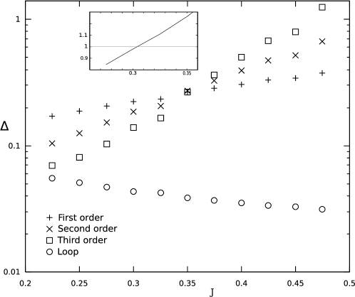
Figure 1: Relative error $\Delta$ (38) on the inferred couplings as a function of the inverse temperature $J$ of the Sherrington-Kirkpatrick model with $N=200$ spins. Monte Carlo simulations are run over 100 steps, and averages and error bars are computed from 100 samples. Top: orders 1,2, 3 of the expansion. Bottom: expression (40) which includes the sum over all loop diagrams. Inset: largest eigenvalue $\Lambda$ of matrix $M$ as a function of $J$.

3.2 Resummation of loop diagrams

The divergence coming from the alternate series can be cured by summing all loop diagrams. A simple inspection shows that each diagram is multiplied by $\pm 1$ depending on the parity of the number of its links. From an algebraic point of view

$$J_{ij}^{*(\text{loop})} = \beta K_{ij}-\beta^{2}\sum_{k}K_{jk}K_{ki}L_{k}+\beta^{3}\sum_{k,l}K_{jk}K_{kl}K_{li}L_{k}L_{l}+...$$ (39)

$$= (L_{i}L_{j})^{-1/2}\left[(\mathbf{M})_{ij}-(\mathbf{M}^{2})_{ij}+(\mathbf{M}^{3})_{ij}-\cdots\right]$$

$$= (L_{i}L_{j})^{-1/2}\left[\mathbf{M}\cdot(\mathrm{Id}+\mathbf{M})^{-1})\right]_{ij}$$

where $\mathbf{M}$ is the matrix defined by $\mathbf{M}_{ij}=\beta K_{ij}\sqrt{L_{i}L_{j}}$ and $\mathbf{M}_{ii}=0$. Expression (39) for the coupling was already known as a consequence of the TAP equations (see [14] and [10]), and is exact up to $O(1/N)$ corrections for infinite range models. Our calculation shows how models with $O(1)$ couplings depart from the TAP expression,

$$J_{ij}^{*}(\{c_{kl}\},\{m_{i}\})=J_{ij}^{*(\text{loop})}-2\beta^{2}m_{i}m_{j}K_{ij}^{2}+\frac{2}{3}\beta^{3}K_{ij}^{3}\left[-1+3m_{i}^{2}+3m_{j}^{2}+3m_{i}^{2}m_{j}^{2}\right]+O(\beta^{4})$$ (40)

Figure 1 shows how the resummation of loop diagrams eliminates the divergence in the relative error $\Delta$ as expected. The same phenomenon takes place in the simpler Curie-Weiss model of a ferromagnet where spins interact through uniform couplings $J_{ij}=J_{0}/N$, and the (connected) correlations are of the same order, $c_{ij}=c/N$. From the relation $Nc=\partial m/\partial h$ we can deduce that the large-$N$ expression for the coupling

$$J_{0}=\frac{c}{1+c}=c-c^{2}+c^{3}-c^{4}+...$$ (41)

is an alternating series with radius of convergence $c=1$. This radius is also given by the condition that the largest eigenvalue of $c_{ij}$ equals 1. This condition applies to the general case too: a necessary condition for the convergence of equation (40) is that the largest eigenvalue $\Lambda$ of $M$ must be smaller than unity. We plot in the Inset of Figure 1 the behavior of $\Lambda$ as a function of $J$. It appears that $\Lambda=1$ for $J\simeq.3$, a value comparable to the intersection point of the lowest order expansions, $J\simeq.35$.

The apparent large value of the relative error $\Delta$ in Figure 1 is not due to the quality of the expansion but to the the noise in the correlations and magnetizations introduced by the imperfect sampling of MC simulations. We show in Figure 2 how the absolute error $J\times\Delta$ decays as the square root of the number of MC steps, and is roughly independent of $J$ (except close to the spin-glass temperature $J=1$). As expected, for an infinite number of MC steps and $N\rightarrow\infty$, the error should vanish.

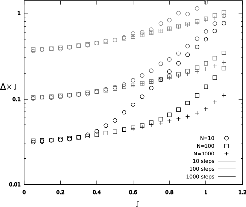
Figure 2: Absolute error $J\times\Delta$ on the inferred couplings as a function of the inverse temperature $J$ of the Sherrington-Kirkpatrick model. Inference is done through formula (40), which takes into account all loop diagrams. The error decreases with the number of spins and the number of Monte Carlo steps (shown on the figure).

3.3 Resummation of two-spin diagrams

Looking carefully at the results of the Section 3.1 one can deduce a general formula for the two spins diagrams,

$$J_{ij}^{*(\text{2-spin})} = K_{ij}-2m_{i}m_{j}K_{ij}^{2}+\frac{1}{3}K_{ij}^{3}(1+3m_{i}^{2})(1+3m_{j}^{2})-4K_{ij}^{4}m_{i}m_{j}(1+m_{i}^{2})(1+m_{j}^{2})$$ (42)

$$+ ...+(-1)^{k}\frac{1}{k-1}K_{ij}^{k-1}\frac{\left\langle(\sigma_{i}-m_{i})^{k}\right\rangle}{1-m_{i}^{2}}\frac{\left\langle(\sigma_{j}-m_{j})^{k}\right\rangle}{1-m_{j}^{2}}+...$$

$$= \frac{1}{4}\ln\left[1+K_{ij}(1+m_{i})(1+m_{j})\right]+\frac{1}{4}\ln\left[1+K_{ij}(1-m_{i})(1-m_{j})\right]$$

$$- \frac{1}{4}\ln\left[1-K_{ij}(1-m_{i})(1+m_{j})\right]-\frac{1}{4}\ln\left[1-K_{ij}(1+m_{i})(1-m_{j})\right]$$

Where we have used equation (111) from Appendix C to evaluate the averages. This expression is exact, and was checked by a symbolic calculation program. Note that in the case of zero magnetization, (42) simplifies to $J_{ij}^{*(\text{2 spins})}=\tanh^{-1}c_{ij}$.

The resummation of all 2-spin diagrams and loop diagrams can be done, with the result

$$J_{ij}^{*(\text{2-spin+loop})}=J_{ij}^{*\text{(loop)}}+J_{ij}^{*\text{(2-spin)}}-\frac{K_{ij}}{1-K_{ij}^{2}L_{i}L_{j}}\ .$$ (43)

The last term in (43) prevents double-counting of diagrams of the type , (obtained through contraction of ), and is derived in Appendix D. The compact expression (43) contains all the diagrams present in (27), in addition to higher order loop and 2-spin contributions.

Resummation of all diagrams with a larger number $k$ of spins is harder. It is done in Section 4.2 in the case of zero magnetizations and $k=3$. For larger values of $k$ we are not aware of any closed analytical expression, and resummation can be done by means of numerical procedures only. An important remark is that contributions from diagrams with $k$ spins behave as $O(\prod_{i=1}^{k}(1-m_{i}^{2}))$ when the $m_{i}$s tend to 1 (or -1) as we show in Appendix C. This expansion is particularly adapted to the inference of couplings from strongly magnetized data; a practical application can be found in [15].

4 Further results in the zero magnetization case

4.1 Higher order expansions of the entropy, couplings, and fields

While the procedure described in Section 2 allows for a systematic expansion of the couplings in powers of $\beta$ it is technically involved to do by hand. In this section we find numerically the expansion up to order $O(\beta^{8})$ in the simpler case where $m_{i}=0$ for all spins $i$.

We know that the expansion of $S$ up to fifth order is given by the sum of all diagrams with 5 links or less. More precisely,

$$S^{\text{(5th order)}} = S^{\text{(4th order)}}+a_{1}\cdot\begin{tabular}[]{c}\includegraphics[scale={.4}]{o5_1.epsi}\end{tabular}+a_{2}\cdot\begin{tabular}[]{c}\includegraphics[scale={.4}]{o5_2.epsi}\end{tabular}+$$ (46)

$$+ a_{3}\cdot\begin{tabular}[]{c}\includegraphics[scale={.4}]{o5_3.epsi}\end{tabular}+a_{4}\cdot\begin{tabular}[]{c}\includegraphics[scale={.4}]{o5_4.epsi}\end{tabular}+a_{5}\cdot\begin{tabular}[]{c}\includegraphics[scale={.4}]{o5_5.epsi}\end{tabular}+\cdots+\mathrm{O}(c^{6})\,.$$ (50)

As we already know $S^{\text{(4th order)}}$ from the previous Section what remains to be found are the $a_{i}$ coefficients. According to the procedure outlined in Section 2 those coefficients are rational (and in particular, for low orders, with a small integer denominator). Our idea is to find those coefficients from a fit of a numerical solution.

Numerically we minimize the entropy (2) for a small number $N$ of spins (not larger than eight). Correlations are arbitrary numbers chosen to be very small (about $10^{-7}$) since we want the corrections of the order of $O(c^{6})$ to be numerically negligible compared to $O(c^{5})$ terms. Of course, when the correlations are very small, so are the inferred couplings. To estimate the latter to sufficient accuracy we have performed our calculations with a unusual large number of decimal units ($\approx 400$). A computer program, at each step $l$, randomly chooses the couplings $c_{ij}^{l}$ and numerically evaluates the corresponding entropy $S_{l}$ and correlations $c_{ij}^{l}$ through an exact enumeration over the $2^{N}$ spin configurations. Then it calculates

$$D=\sum_{l=1}^{L}\left[S_{l}-S^{\text{(5th order)}}(c_{ij}^{l})\right]^{2}$$ (51)

over a large number $L$ of random samples. This quantity is quadratic in the coefficients $a_{i}$, so its minimum can be easily obtained, and we could deduce that the coefficients in the expansion (46) are all zero. Using this procedure, order by order, we have determined the following expansion for $J_{ij}^{*}$ (where the coefficients found numerically differed from the rational fractions listed below by less than $10^{-10}$):

$$J_{ij}^{*} = J_{ij}^{*\text{(2-spin+loop)}}+\begin{tabular}[]{c}\includegraphics[scale={.4}]{loop_d2_p.epsi}\end{tabular}-\frac{4}{3}\begin{tabular}[]{c}\includegraphics[scale={.4}]{o7_p1.epsi}\end{tabular}-4\left(\begin{tabular}[]{c}\includegraphics[scale={.4}]{o7_p2_ij.epsi}\end{tabular}+\begin{tabular}[]{c}\includegraphics[scale={.4}]{o7_p3_ij.epsi}\end{tabular}\right)$$ (56)

$$+ 2\left(\begin{tabular}[]{c}\includegraphics[scale={.4}]{3spins_lin2_p1_ij.epsi}\end{tabular}+\begin{tabular}[]{c}\includegraphics[scale={.4}]{3spins_lin2_p2_ij.epsi}\end{tabular}\right)+16\begin{tabular}[]{c}\includegraphics[scale={.4}]{o8_3_p1.epsi}\end{tabular}+8\left(\begin{tabular}[]{c}\includegraphics[scale={.4}]{o8_3_p2_ij.epsi}\end{tabular}+\begin{tabular}[]{c}\includegraphics[scale={.4}]{o8_3_p3_ij.epsi}\end{tabular}\right)$$ (62)

$$- 2\begin{tabular}[]{c}\includegraphics[scale={.4}]{loop_d3_p.epsi}\end{tabular}-4\begin{tabular}[]{c}\includegraphics[scale={.4}]{o8_2_p1.epsi}\end{tabular}-4\begin{tabular}[]{c}\includegraphics[scale={.4}]{o8_2_p2.epsi}\end{tabular}+O(c^{8})$$ (66)

We can note the absence of any term with five or more spins in this expansion. We suspect that the lowest order diagram in this expansion for a given number spins is the loop with double links. In particular, the first diagram with five spins would be , which is not present in (66) since it is $O(c^{9})$.

4.2 Three spins summation for zero magnetization

For three spins and zero magnetizations the entropy (2) can be minimized exactly with a symbolic algebra program, with the following results for the couplings

$$J_{ij}^{*\text{(3-spin)}}=\frac{1}{4}\sum_{k\,(\neq i,j)} \left\{\log\left[\frac{1+c_{ij}-c_{ik}-c_{jk}}{1-c_{ij}-c_{ik}+c_{jk}}\right]\right.$$ (67)

$$- \left.\log\left[\frac{1-c_{ij}+c_{ik}-c_{jk}}{1-c_{ij}-c_{ik}+c_{jk}}\right]+\log\left[\frac{1+c_{ij}+c_{ik}+c_{jk}}{1-c_{ij}-c_{ik}+c_{jk}}\right]\right\}$$

Following the same lines as in Section 3.3 we gather our previous results in the $m_{i}=0$ case under the form,

$$J_{ij}^{*\text{(2-spin+loop+3-spin)}} = J_{ij}^{*\text{(2-spin+loop)}}+J_{ij}^{*\text{(3-spin)}}$$ (68)

$$- \sum_{k\,(\neq i,j)}\left\{J_{ij}^{*\text{(2 spins)}}+\frac{c_{ij}-c_{ik}c_{jk}}{1-c_{ij}^{2}-c_{ik}^{2}-c_{jk}^{2}+2c_{ij}c_{jk}c_{ki}}-\frac{c_{ij}}{1-c_{ij}^{2}}\right\}\,.$$

4.3 Check on the one-dimensional Ising model

We consider a unidimensional Ising model with uniform coupling $J$ between nearest neighbours. We have

$$c_{ij}=\left|\tanh J\right|^{|i-j|}$$ (69)

$$J_{ij}^{*\text{(2-spin)}}=\tanh^{-1}\bigg{(}\left|\tanh J\right|^{|i-j|}\bigg{)}$$ (70)

We can see from the above formula that the sum of all 2-spin diagrams infer the correct value of the couplings $J_{i,i+1}$, but give a non-zero value for the other ones. We can also evaluate the sum of loop diagrams (with $c=\tanh J$):

$$J_{ij}^{*\text{(loop)}}=\frac{c}{1-c^{2}}(\delta_{i,i+1}+\delta_{i,i-1})\,,$$ (71)

where $\delta_{i,j}$ is the Kronecker function. We obtain a zero contribution for non-neighbouring sites, but an erroneous values for the nearest-neighbour coupling $J_{i,i+1}$. If we consider the contributions from both 2-spin and loop diagrams,

$$J_{ij}^{\text{(2-spin+loop)}} = J(\delta_{i,i+1}+\delta_{i,i-1})+\left[\tanh c_{ij}-\frac{c_{ij}}{1-c_{ij}^{2}}\right](1-\delta_{i,i+1})(1-\delta_{i,i-1})$$ (72)

$$= J(\delta_{i,i+1}+\delta_{i,i-1})+O(c^{6})\ ,$$

which is correct to the order $c^{6}$. The next contribution to the couplings coming from the expansion (66) corresponds to , whose leading term is indeed proportional to $c_{i,i+2}\cdot c_{i,i+1}^{2}\cdot c_{i+1,i+2}^{2}=c^{6}$.

We may also want to understand how $J_{i,i+2}$ converges to zero. Using geometric series calculations one can evaluate

$$\begin{tabular}[]{c}\includegraphics[scale={.4}]{alphabeta.epsi}\end{tabular}=c^{2\gamma+\alpha+\beta}\cdot\frac{1+c^{2\alpha}+c^{2\beta}}{1-c^{\alpha+\beta}}$$ (74)

$$\begin{tabular}[]{c}\includegraphics[scale={.4}]{loop_d3_p.epsi}\end{tabular}=2c^{10}\frac{1+c^{4}}{1-c^{4}}+c^{14}\frac{2+c^{8}}{(1-c^{4})^{2}}$$ (76)

Performing the whole summation in (66) we find that $J_{i,i+2}=O(c^{8})$, which is consistent with the first missing contribution from the expansion, .

4.4 Application to the Sherrington-Kirkpatrick model

We have seen above that the error on the inferred couplings for the Sherrington-Kirpatrick model is essentially due to the noise in the MC estimates of the correlations and magnetizations. To avoid this source of noise we now evaluate the error due to our truncated expansion using a program that calculates $c_{ij}$ through an exact enumeration of all $2^{N}$ spin configurations. We are limited to small values of $N$ (10, 15 and 20). However the case of a small number of spins is particularly interesting because, for the SK model, the summation of loop diagrams is exact in the limit $N\rightarrow\infty$. The importance of terms in our expansions not included in the loop resummation is thus better studied at small N.

Results are shown in Figure 3. The error is remarkably small for weak couplings, and get dominated by finite-digit accuracy ($10^{-13}$) in this limit. Not surprisingly it behaves better than simple loop resummation, and also outperforms the message-passing-based method recently introduced in [7].

Figure 3: Relative error $\Delta$ (38) as a function of $J$ for the SK model for our resummation $J_{ij}^{\text{(2 spin + loop + 3 spin)}}$ (68) compared to the Susceptibility Propagation method of Mézard and Mora [7] and loop resummation $J_{ij}^{\text{(loop)}}$ (40).

5 Perspectives

As we saw in Sections 4.3 and 4.4 the expansion method introduced in this paper works well for both the Sherrington-Kirkpatrick sping-glass –an infinite dimensional system, with very dilute couplings– and the unidimensional Ising –with only a few but strong couplings per site– models. It would be interesting to investigate how accurate our method is for ‘Small-World’-like interaction networks, which have both kinds of couplings [16].

In principle the assumption of binary-valued spins ($\sigma_{i}=\pm 1$) is not central to our expansion and could be straightforwardly released to tackle the case of Potts models, where each spin can be in $q$ possible states ($\sigma_{i}=1,...,q$). Such a generalization would make the method useful to connect with biological problems involving amino-acids [5].

Finally our expansion breaks down with the onset of the spin-glass phase as can be seen from Figure 3. The failure of our method (and of other existing algorithms) is not surprising. Correlations and magnetizations have a physical meaning when there is a single pure state. In presence of more than one phases Gibbs averages have indirect significance. A well-known example is the ferromagnet at low temperature and zero field where two equally-likely phases of opposite magnetizations $\pm m_{s}$ exist, and the resulting Gibbs magnetization $m$ truly vanishes (for any finite $N$). Work is in progress to extend our expansion technique to this multiple-phase regime.

Acknowledgments: We are grateful to S. Cocco and S. Leibler for very useful and insightful discussions. We also thank S. C. for the critical reading of the manuscript. This work was partially funded by the Agence Nationale de la Recherche JCJC06-144328 and the Galileo 17460QJ contracts.

Appendix A Details of the small-$\beta$ expansion

Let $O$ be an observable of the spin configuration (which can explicitly depend on the inverse temperature $\beta$), and

$$\left\langle O\right\rangle=\frac{1}{Z}\operatorname*{Tr}_{\{\sigma_{i}\}}O\;e^{U}$$ (77)

its average value, where $U$ is defined in (6), and $Z=\exp(\tilde{S})$. The derivative of the average value of $O$ fulfills the following identity,

$$\frac{\partial\left\langle O\right\rangle}{\partial\beta}=\frac{1}{Z}\operatorname*{Tr}_{\{\sigma_{i}\}}\left[\frac{\partial O}{\partial\beta}+O\frac{\partial U}{\partial\beta}\right]e^{U}-\frac{1}{Z^{2}}\frac{\partial Z}{\partial\beta}\operatorname*{Tr}_{\{\sigma_{i}\}}Oe^{U}=\left\langle\frac{\partial O}{\partial\beta}\right\rangle+\left\langle O\frac{\partial U}{\partial\beta}\right\rangle$$ (78)

where the term in $Z^{-2}$ vanishes as a consequence of (9).

A.1 First order expansion

Using (78) and (9),

$$0=\frac{\partial^{2}\tilde{S}}{\partial\beta^{2}}=\frac{\partial}{\partial\beta}\left\langle\frac{\partial U}{\partial\beta}\right\rangle=\left\langle\frac{\partial^{2}U}{\partial\beta^{2}}\right\rangle+\left\langle\left(\frac{\partial U}{\partial\beta}\right)^{2}\right\rangle$$ (79)

and by using the explicit form of $U$ given in (6):

$$\left.\frac{\partial^{2}\tilde{S}}{\partial\beta^{2}}\right|_{0}=-\sum_{i<j}c_{ij}\left.\frac{\partial J_{ij}^{*}}{\partial\beta}\right|_{0}+\sum_{i<j}\left(\left.\frac{\partial J_{ij}^{*}}{\partial\beta}\right|_{0}\right)^{2}(1-m_{i}^{2})(1-m_{j}^{2})+\sum_{i}\left(\left.\frac{\partial\lambda_{i}^{*}}{\partial\beta}\right|_{0}\right)^{2}(1-m_{i}^{2})$$ (80)

In Appendix B we show that $\left.\frac{\partial\lambda_{i}^{*}}{\partial\beta}\right|_{0}=0$. As $\tilde{S}$ is constant we end up with the following algebraic equation for the first order derivative of $J_{ij}^{*}(\beta)$,

$$0=-\sum_{i<j}c_{ij}\left.\frac{\partial J_{ij}^{*}}{\partial\beta}\right|_{0}+\sum_{i<j}\left(\left.\frac{\partial J_{ij}^{*}}{\partial\beta}\right|_{0}\right)^{2}(1-m_{i}^{2})(1-m_{j}^{2})\ .$$ (81)

The only non-zero solution of the above equation, symmetric under index permutations, is the announced result (11).

A.2 Second order expansion

Using (78) and (79)

$$0=\frac{\partial^{3}\tilde{S}}{\partial\beta^{3}}=\frac{\partial}{\partial\beta}\left[\left\langle\frac{\partial^{2}U}{\partial\beta^{2}}\right\rangle+\left\langle\left(\frac{\partial U}{\partial\beta}\right)^{2}\right\rangle\right]=\left\langle\frac{\partial^{3}U}{\partial\beta^{3}}\right\rangle+3\left\langle\frac{\partial^{2}U}{\partial\beta^{2}}\frac{\partial U}{\partial\beta}\right\rangle+\left\langle\left(\frac{\partial U}{\partial\beta}\right)^{3}\right\rangle$$ (82)

A straightforward calculation gives (where we omit for clarity the notation $|_{0}$ and the ^∗ subscript from $J_{ij}$ and $\lambda_{i}$)

$$\left\langle\frac{\partial^{3}U}{\partial\beta^{3}}\right\rangle_{0} = -2\sum_{i<j}\frac{\partial^{2}J_{ij}}{\partial\beta^{2}}c_{ij}$$ (83)

$$\left\langle\frac{\partial^{2}U}{\partial\beta^{2}}\frac{\partial U}{\partial\beta}\right\rangle_{0} = \sum_{i<j}\frac{\partial^{2}J_{ij}}{\partial\beta^{2}}\frac{\partial J_{ij}}{\partial\beta}L_{i}L_{j}+\sum_{i}\frac{\partial^{2}\lambda_{i}}{\partial\beta^{2}}\frac{\partial\lambda_{i}}{\partial\beta}L_{i}$$ (84)

$$\left\langle\left(\frac{\partial U}{\partial\beta}\right)^{3}\right\rangle_{0} = 6\sum_{i<j<k}\frac{\partial J_{ij}}{\partial\beta}\frac{\partial J_{jk}}{\partial\beta}\frac{\partial J_{ki}}{\partial\beta}L_{i}L_{j}L_{k}+$$ (85)

$$+ \sum_{i<j}\left(\frac{\partial J_{ij}}{\partial\beta}\right)^{3}4m_{i}m_{j}L_{i}L_{j}+6\sum_{i<j}\frac{\partial J_{ij}}{\partial\beta}\frac{\partial\lambda_{i}}{\partial\beta}\frac{\partial\lambda_{j}}{\partial\beta}L_{i}L_{j}$$

Using (82), results from Appendix B for the expressions of the derivatives of $\lambda_{i}$ in $\beta=0$, and (11) we obtain (10) for $k=3$ with

$$Q_{2}=-4\sum_{i<j}\frac{c_{ij}^{3}m_{i}m_{j}}{(1-m_{i}^{2})^{2}(1-m_{j}^{2})^{2}}-6\sum_{i<j<k}\frac{c_{ij}c_{jk}c_{ki}}{(1-m_{i}^{2})(1-m_{j}^{2})(1-m_{k}^{2})}$$ (86)

from which we deduce

$$\left.\frac{\partial^{3}S}{\partial\beta^{3}}\right|_{0}=4\sum_{i<j}K_{ij}^{3}m_{i}m_{j}L_{i}L_{j}+6\sum_{i<j<k}K_{ij}K_{jk}K_{ki}L_{i}L_{j}L_{k}$$ (87)

and

$$\left.\frac{\partial^{2}J_{ij}}{\partial\beta^{2}}\right|_{0}=-4m_{i}m_{j}K_{ij}^{2}-2\sum_{k(\neq i,\,\neq j)}K_{jk}K_{ki}L_{k}\ .$$ (88)

A.3 Third order expansion

The procedure to derive the third order expansion for the coupling is identical to the second order one. We start from

$$0=\frac{\partial^{4}\tilde{S}}{\partial\beta^{4}}=\left\langle\frac{\partial^{4}U}{\partial\beta^{4}}\right\rangle+3\left\langle\left(\frac{\partial^{2}U}{\partial\beta^{2}}\right)^{2}\right\rangle+4\left\langle\frac{\partial^{3}U}{\partial\beta^{3}}\frac{\partial U}{\partial\beta}\right\rangle+6\left\langle\left(\frac{\partial U}{\partial\beta}\right)^{2}\frac{\partial^{2}U}{\partial\beta^{2}}\right\rangle+\left\langle\left(\frac{\partial U}{\partial\beta}\right)^{4}\right\rangle$$ (89)

and evaluate each term in the sum:

$$\left\langle\frac{\partial^{4}U}{\partial\beta^{4}}\right\rangle_{0} = -3\sum_{i<j}\left.\frac{\partial^{3}J_{ij}}{\partial\beta^{3}}\right|_{0}K_{ij}L_{i}L_{j}$$ (90)

$$\left\langle\left(\frac{\partial^{2}U}{\partial\beta^{2}}\right)^{2}\right\rangle_{0} = \sum_{i<j}\left(\frac{\partial^{2}J_{ij}}{\partial\beta^{2}}\right)^{2}L_{i}L_{j}+\sum_{i}\left(\frac{\partial^{2}\lambda_{i}}{\partial\beta^{2}}\right)^{2}L_{i}+\left[\sum_{i<j}K_{ij}^{2}L_{i}L_{j}\right]^{2}$$ (91)

$$\left\langle\frac{\partial^{3}U}{\partial\beta^{3}}\frac{\partial U}{\partial\beta}\right\rangle_{0} = \sum_{i<j}K_{ij}\frac{\partial^{3}J_{ij}}{\partial\beta^{3}}L_{i}L_{j}$$ (92)

$$\left\langle\left(\frac{\partial U}{\partial\beta}\right)^{2}\frac{\partial^{2}U}{\partial\beta^{2}}\right\rangle_{0} = 2\sum_{i<k}\sum_{j}K_{ij}K_{jk}\frac{\partial^{2}J_{ki}}{\partial\beta^{2}}L_{i}L_{j}L_{k}+4\sum_{i<j}K_{ij}^{2}\frac{\partial^{2}J_{ij}}{\partial\beta^{2}}m_{i}m_{j}L_{i}L_{j}$$ (93)

$$+ \sum_{i}\sum_{j}K_{ij}^{2}\frac{\partial^{2}\lambda_{i}}{\partial\beta^{2}}(-2m_{i})L_{i}L_{j}-\left\langle\left(\frac{\partial U}{\partial\beta}\right)^{2}\right\rangle_{0}\sum_{i<j}K_{ij}^{2}L_{i}L_{j}$$

$$\left\langle\left(\frac{\partial U}{\partial\beta}\right)^{4}\right\rangle_{0} = \sum_{i<j}K_{ij}^{4}(3m_{i}^{2}+1)L_{i}(3m_{j}^{2}+1)L_{j}+3\sum_{i<j,\,k<l\,(k\neq i,\,l\neq j)}K_{ij}^{2}K_{kl}^{2}L_{i}L_{j}L_{k}L_{l}+$$ (94)

$$+ 6\sum_{i<k}\sum_{j}K_{ij}^{2}K_{jk}^{2}(3m_{j}^{2}+1)L_{i}L_{j}L_{k}+$$

$$+ 12\sum_{i<j<k}K_{ij}K_{jk}K_{ki}L_{i}L_{j}L_{k}\left[4m_{i}m_{j}K_{ij}+4m_{i}m_{k}K_{ik}+4m_{k}m_{i}K_{ki}\right]+$$

$$+ 3\sum_{i,j,k,l\,(\neq)}K_{ij}K_{jk}K_{kl}K_{li}L_{i}L_{j}L_{k}L_{l}$$

Using the results from Appendix B we can write all the terms above in the same form

$$-3\left[\sum_{i<j}K_{ij}^{2}L_{i}L_{j}\right]^{2} = -3\sum_{i<j,\,k<l\,(k\neq i,\,l\neq j)}K_{ij}^{2}K_{kl}^{2}L_{i}L_{j}L_{k}L_{l}$$ (95)

$$- 6\sum_{i<j}\sum_{k}K_{ik}^{2}K_{kj}^{2}L_{i}L_{j}L_{k}^{2}-3\sum_{i<j}K_{ij}^{4}L_{i}^{2}L_{j}^{2}$$

$$12\sum_{i<j}\sum_{k}K_{ik}K_{kj}\frac{\partial^{2}J_{ij}}{\partial\beta^{2}}L_{i}L_{j}L_{k} = -48\sum_{i<j}\sum_{k}K_{ij}^{2}K_{ik}K_{kj}m_{i}m_{j}L_{i}L_{j}L_{k}-$$ (96)

$$- 12\sum_{i,j,k,l\,(\neq)}K_{ij}K_{jk}K_{kl}K_{li}L_{i}L_{j}L_{k}L_{l}$$

$$- 24\sum_{i<j}\sum_{k}K_{ik}^{2}K_{kj}^{2}L_{i}L_{j}L_{k}^{2}$$

$$\sum_{i<j}K_{ij}^{2}\frac{\partial^{2}J_{ij}}{\partial\beta^{2}}m_{i}m_{j}L_{i}L_{j} = -4\sum_{i<j}K_{ij}^{4}m_{i}^{2}m_{j}^{2}L_{i}L_{j}-2\sum_{i<j}\sum_{k}K_{ij}^{2}K_{jk}K_{ki}m_{i}m_{j}L_{i}L_{j}L_{k}$$ (97)

$$3\sum_{i<j}\left(\frac{\partial^{2}J_{ij}}{\partial\beta^{2}}\right)^{2}L_{i}L_{j} = 48\sum_{i<j}K_{ij}^{4}m_{i}^{2}m_{j}^{2}L_{i}L_{j}+48\sum_{i<j}\sum_{k}K_{ij}^{2}K_{ik}K_{kj}m_{i}m_{j}L_{i}L_{j}L_{k}+$$ (98)

$$+ 6\sum_{i,j,k,l\,(\neq)}K_{ij}K_{jk}K_{kl}K_{li}L_{i}L_{j}L_{k}L_{l}$$

$$+ 12\sum_{i<j}\sum_{k}K_{ik}^{2}K_{kj}^{2}L_{k}^{2}L_{i}L_{j}$$

$$6\sum_{i}\sum_{j}K_{ij}^{2}\frac{\partial^{2}\lambda_{i}}{\partial\beta^{2}}(-2m_{i})L_{i}L_{j} = -24\sum_{i}\sum_{j}K_{ij}^{4}m_{i}^{2}(1-m_{j}^{2})L_{i}L_{j}$$ (99)

$$- 48\sum_{i<j}\sum_{k}K_{ik}^{2}K_{kj}^{2}m_{k}^{2}L_{i}L_{j}L_{k}$$

$$3\sum_{k}\left(\frac{\partial^{2}\lambda_{k}}{\partial\beta^{2}}\right)^{2}L_{k} = 24\sum_{i<j}\sum_{k}K_{ik}^{2}K_{kj}^{2}m_{k}^{2}L_{i}L_{j}L_{k}+12\sum_{i}\sum_{j}K_{ij}^{4}m_{i}^{2}L_{i}L_{j}^{2}$$ (100)

Again we find equation (10) with

$$Q_{3} = -\sum_{i<j}K_{ij}^{4}\left[(3m_{i}^{2}+1)(3m_{j}^{2}+1)-48m_{i}^{2}m_{j}^{2}\right]L_{i}L_{j}$$ (101)

$$+ 12\sum_{i<j}\sum_{k}K_{ik}^{2}K_{jk}^{2}L_{i}L_{j}L_{k}^{2}+3\sum_{i,j,k,l\,(\neq)}K_{ij}K_{jk}K_{kl}K_{li}L_{i}L_{j}L_{k}L_{l}$$

$$+ 12\sum_{i}\sum_{j}K_{ij}^{4}m_{i}^{2}L_{i}L_{j}^{2}+3\sum_{i<j}K_{ij}^{4}L_{i}^{2}L_{j}^{2}$$

which gives the fourth order contribution to the entropy,

$$\frac{\partial^{4}S}{\partial\beta^{4}} = -2\sum_{i<j}K_{ij}^{4}\left[1+3m_{i}^{2}+3m_{j}^{2}+9m_{i}^{2}m_{j}^{2}\right]L_{i}L_{j}-12\sum_{i<j}\sum_{k}K_{ik}^{2}K_{kj}^{2}L_{k}^{2}L_{i}L_{j}$$ (102)

$$- 24\sum_{i<j<k<l}(K_{ij}K_{jk}K_{kl}K_{li}+K_{ik}K_{kj}K_{lj}K_{il}+K_{ij}K_{jl}K_{lk}K_{ki})L_{i}L_{j}L_{k}L_{l}$$

and the third order contribution to the coupling,

$$\left.\frac{\partial^{3}J_{ij}}{\partial\beta^{3}}\right|_{0} = 2K_{ij}^{3}\left[1+3m_{i}^{2}+3m_{j}^{2}+9m_{i}^{2}m_{j}^{2}\right]+6\sum_{k\,(\neq i,\,\neq j)}K_{ij}(K_{jk}^{2}L_{j}+K_{ki}^{2}L_{i})L_{k}+$$ (103)

$$+ 6\sum_{\begin{subarray}{c}k,l\\ (k\neq i,l\neq j)\end{subarray}}K_{jk}K_{kl}K_{li}L_{k}L_{l}\,.$$

Appendix B Derivatives of $\lambda^{*}_{i}$ in $\beta=0$

Since $m_{i}$ and $h_{i}$ are conjugated thermodynamic variables it is natural to evaluate

$$\frac{\partial\tilde{S}}{\partial m_{k}} = \left\langle\frac{\partial U}{\partial m_{k}}\right\rangle=\sum_{i<j}c_{ij}\int_{0}^{\beta}\mathrm{\;d}\beta^{\prime}\frac{\partial J_{ij}^{*}(\beta^{\prime})}{\partial m_{k}}$$ (104)

$$- \sum_{i<j}J_{ij}^{*}(\beta)\left\langle(\sigma_{i}-m_{i})\delta_{jk}+(\sigma_{j}-m_{j})\delta_{ik}\right\rangle+\sum_{i<j}\frac{\partial J_{ij}^{*}}{\partial m_{k}}\left\langle(\sigma_{i}-m_{i})(\sigma_{j}-m_{j})\right\rangle-\lambda_{k}^{*}(\beta)$$

$$= -\lambda_{k}^{*}(\beta)+\sum_{i<j}c_{ij}\int_{0}^{\beta}\mathrm{\;d}\beta^{\prime}\frac{\partial J_{ij}^{*}(\beta^{\prime})}{\partial m_{k}}$$

As the modified entropy is independent of $\beta$,

$$\frac{\partial\tilde{S}}{\partial m_{k}}=\left.\frac{\partial\tilde{S}}{\partial m_{k}}\right|_{0}=-\lambda_{k}^{*}(0)={\tanh}^{-1}(m_{k})=\frac{1}{2}\ln\left(\frac{1+m_{k}}{1-m_{k}}\right)$$ (105)

where we used the well-known result for the entropy of uncorrelated spins. We can then deduce the formula, valid for any $\beta$:

$$\lambda_{k}^{*}(\beta)=\frac{1}{2}\ln\left(\frac{1-m_{k}}{1+m_{k}}\right)+\sum_{i<j}c_{ij}\int_{0}^{\beta}\mathrm{\;d}\beta^{\prime}\frac{\partial J_{ij}^{*}(\beta^{\prime})}{\partial m_{k}}\ .$$ (106)

It is now straightforward to deduce the expansion of $\lambda_{i}^{*}$ to the order $O(\beta^{k})$ from the expansion of $J_{ij}^{*}$ to the order $O(\beta^{k-1})$. In particular,

$$\left.\frac{\partial\lambda_{k}^{*}}{\partial\beta}\right|_{0}=0$$ (107)

and using the order $O(\beta)$ of the $J_{ij}^{*}$ expansion,

$$\left.\frac{\partial^{2}\lambda_{k}^{*}}{\partial\beta^{2}}\right|_{0}=2m_{k}\sum_{i}K_{ik}^{2}L_{i}\,.$$ (108)

Appendix C Large magnetization expansion

Equation (27) suggests that to expand $J_{ij}^{*}$ to the order of $(L_{i})^{k}$ one has to sum all the diagrams with up to $k+2$ spins. This statement is true if the expansion for $J_{ij}^{*}$ is of the form

$$J_{ij}^{*}=A_{ij}+\sum_{k}L_{k}A_{ijk}+\sum_{k}\sum_{l}L_{k}L_{l}A_{ijkl}+...$$ (109)

where the coefficients $A_{i_{1}i_{2}...i_{n}}$ are polynomials in the couplings $K_{i_{\alpha}i_{\beta}}$ and the magnetizations $m_{\alpha}$ ($\alpha,\beta<n$). In the following we will show that the above statement is true to any order of the expansion in $\beta$ by recurrence. First of all, from (106) we see that if $J_{ij}^{*}$ is of the form (109) up to the order $k$, so is $\lambda_{i}^{*}$ to the same order.

As we saw in section 2, to find an equation for $\frac{\partial^{k}S}{\partial\beta^{k}}$, one must evaluate $\frac{\partial^{k+1}\tilde{S}}{\partial\beta^{k+1}}$. Using Eq. 78, we can write

$$\frac{\partial^{k+1}\tilde{S}}{\partial\beta^{k+1}}=\left\langle\left(\frac{\partial}{\partial\beta}+\frac{\partial U}{\partial\beta}\right)^{k}\frac{\partial U}{\partial\beta}\right\rangle=\sum_{\{\alpha\}}P_{\alpha}\left\langle\prod_{j=1}^{k+1}\frac{\partial^{\alpha_{j}}U}{\partial\beta^{\alpha_{j}}}\right\rangle$$ (110)

where $\alpha$ is a multi-index and $|\alpha|=k+1$, and $P_{\alpha}$ a multiplicity coefficient. The highest order term of this expression evaluates to $\sum_{ij}L_{i}L_{j}K_{ij}\frac{\partial^{j}J_{ij}^{*}}{\partial\beta^{j}}=\frac{\partial^{k}S}{\partial\beta^{k}}$.

Due to the structure of $U$, spin dependence in (110) will come either from the lower derivatives of $J_{ij}^{*}$ (of the form (109) by hypothesis), from the derivatives of $\lambda_{i}^{*}$, or explicitly from $U$. In the later case we get a multiplicative factor $(\sigma_{i}-m_{i})$. Hence we end up with computing a term, with $k\geq 1$, of the form

$$\left\langle(\sigma_{i}-m_{i})^{k}\right\rangle=(-1)^{k}(1-m_{i}^{2})\frac{(m+1)^{k-1}-(m-1)^{k-1}}{2}$$ (111)

Clearly any term including $(\sigma_{i}-m_{i})$ will give a multiplicative factor $L_{i}$ after averaging. As spins are decoupled in the $\beta=0$ limit we obtain the product of those factors over the spins in the diagram as claimed.

Appendix D Double-counting

We want to remove two-spin diagrams from the resummation of loop diagrams. These two-spin diagrams are precisely the ones appearing in the loop diagrams in a system including two spins only. In the case of $N=2$ spins the matrix $M$ reads

$$\mathbf{M}=\beta\left(\begin{array}[]{cc}0&K_{ij}\sqrt{L_{i}L_{j}}\\ K_{ij}\sqrt{L_{i}L_{j}}&0\end{array}\right)\ .$$ (112)

We then calculate $J_{ij}^{*(\text{loop})}$ for this simple $N=2$ spin model from formula (39), and get this way the contribution to be subtracted to the sum of 2-spin and loop diagrams (third term in (43)).

References

- [1] E. Marinari, G. Parisi and J. J. Ruiz-Lorenzo, Numerical Simulations of Spin Glass Systems in Spin Glasses and Random Fields, edited by A. P. Young (World Scientific, Singapore, 1998).
- [2] D. McKay, Information Theory, Inference, and Learning Algorithms, Cambridge University Press (2003).
- [3] E. Schneidman, M.J. Berry, R. Segev, W. Bialek, Nature 440, 1007 (2006);
- [4] J. Shlens et al. J. Neurosci. 26, 8254 (2006).
- [5] M. Socolich, S.W. Lockless, W.P. Russ, H. Lee, K.H. Gardner, R. Ranganathan, Nature 437, 512 (2005).
- [6] Z. Szallasi, Pacific Symposium on Biocomputing 4, 5 (1999).
- [7] M. Mézard, T. Mora, Tauc Conference on Complexity in Neural Network Dynamics (2007).
- [8] J. P. Hansen, I. R. McDonald, Theory of Simple Liquids, (Academic Press, 1976).
- [9] C. De Dominicis, P. C. Martin, J. Math. Phys. 5, 31 (1964)
- [10] T. Plefka, J. Phys. A 15, 1971 (1982).
- [11] A. Georges, J. Yedidia, J. Phys. A 24, 2173 (1991).
- [12] A. Georges, LECTURES ON THE PHYSICS OF HIGHLY CORRELATED ELECTRON SYSTEMS VIII: Eighth Training Course in the Physics of Correlated Electron Systems and High-Tc Superconductors 715, 3 (2004).
- [13] D. Sherringtion, S. Kirkpatrick, Phys. Rev. Lett. 35, 1792 (1975).
- [14] D.J. Thouless, P.W. Anderson, R.G. Palmer, Phil. Mag. 35, 593 (1977).
- [15] S. Cocco, S. Leibler, R. Monasson, preprint (2008).
- [16] D.J. Watts, S.H. Strogatz, Nature 393, 409 (1998).