Particle-acceleration timescales in TeV blazar flares

Abstract

Observations of minute-scale flares in TeV Blazars place constraints on particle acceleration mechanisms in those objects. The implications for a variety of radiation mechanisms have been addressed in the literature; in this paper we compare four different acceleration mechanisms: diffusive shock acceleration, second-order Fermi, shear acceleration and the converter mechanism. When the acceleration timescales and radiative losses are taken into account, we can exclude shear acceleration and the neutron-based converted mechanism as possible acceleration processes in these systems. The first-order Fermi process and the converter mechanism working via SSC photons are still practically instantaneous, however, provided sufficient turbulence is generated on the timescale of seconds. We propose stochastic acceleration as a promising candidate for the energy-dependent time delays in recent gamma-ray flares of Markarian 501.

1 Introduction

Rapid TeV variability has recently been observed by the HESS and MAGIC telescopes in two blazars; PKS 2155–304 (Aharonian et al., 2007) and Markarian 501 (Albert et al., 2007). The timescales of a few minutes are shorter, by at least an order of magnitude, than the light crossing time of the central black hole with a mass of order $M=10^{9}\,{\rm M}_{\odot}$. This suggests that the variability is associated with small regions of the highly relativistic jet rather than the central region, although the latter possibility cannot be completely excluded. Begelman et al. (2008) have examined the constraints that these observations place on the size and location of the emitting region. With an observed variability timescale $t_{\rm var}$ and a jet Lorentz factor $\Gamma$, the flare, if it moves out with the flow, occurs at a distance greater than $ct_{\rm var}\Gamma^{2}$. For $\Gamma\sim 50$ (Begelman et al., 2008) and minute timescale variability this places the flaring region at a distance in excess of one hundred Schwarzschild radii ($r_{S}$) from the central black hole. The relativistic particles that are ultimately responsible for the emission are then required to have been ejected from the central region along with the jet, and subsequently survived out to $100\,r_{S}$ where they then radiate away their energy quickly, or alternatively the particles are accelerated within the jet itself, close to the emission region. In this paper we examine the latter possibility and compare the predicted acceleration timescales for four acceleration mechanisms with the requirements for producing a minute timescale flare.

There are three fundamental questions that we address in this paper. Firstly, we want to see whether particle acceleration could be considered instantaneous on the flaring timescale; is it realistic to assume a fully-developed power-law injection spectrum at the onset of flaring? Related to this question is whether we can exclude particular acceleration mechanisms on the grounds that they are too slow. Secondly, we are interested to see if we can find a set of parameters for which only cooling would be present. If we assume a given input spectrum for particles in a blob travelling with the jet, can we expect further acceleration to be always present? Alternatively, is it more likely that within minute to hour timescales particles would only lose their energy instead of being able to continue accelerating on the same timescales? Finally, can any of the mechanisms work on timescales comparable to the lags between lower- and higher-energy radiation observed in some objects, and what mechanisms could explain the acceleration of particles on the timescale of minutes?

In Section 2 we discuss four possible acceleration mechanisms and their associated timescales. These are (i) first-order Fermi acceleration, (ii) second-order Fermi, (iii) acceleration in a shear flow and (iv) the converter mechanism. The role played by radiation mechanism and loss timescales are then compared with the acceleration properties in Section 3.

2 Acceleration timescales

When particles are scattered by magnetic fluctuations, they gain energy whenever two subsequent scattering centres are moving toward each other, leading to a “head-on” collision. Suitable conditions are provided around a shock wave, where a relativistic particle crossing the shock always sees the plasma – and thus the scattering centres – of the flow on the other side of the shock, approaching. Similarly, relative motion of the scattering centres (Alfvén waves, for example) inside a constant-velocity plasma, moving in different directions, are more often seen as approaching than receding, leading to average gain in energy. The average energy gain during a crossing cycle, and the duration of such a cycle, determines the energy gain rate, $<{\rm d}\gamma/{\rm d}t>$, and the acceleration timescale $\tau\equiv\gamma/\left<{\rm d}\gamma/{\rm d}t\right>$.

The timescale determines how long it takes for a particle with Lorentz factor $\gamma$ to gain or lose energy, allowing easy comparison between the efficiencies of different gain and loss mechanisms. For easily comparable and general results we assume the acceleration to take place in a region with a characteristic, comoving spatial scale $R$, with plasma flow having Lorentz factor $\Gamma$. Particles are assumed to be scattered by irregularities in large-scale magnetic field (with strength $B$) with the average free path between scattering, $\lambda$, being equal to the particle gyroradius $r_{g}$.

2.1 First-order Fermi acceleration

The first-order process takes place at the shock front, where the accelerating particles gain energy by crossing and re-crossing the shock. An average cycle increases the particle energy by a factor of $\Gamma^{2}$ for the first cycle, and by a factor of $\sim 2$ thereafter. The duration of such a cycle, as well as the probability for a particle to be injected into one, depends heavily on the details of the scattering of the particles in the turbulent plasma and the geometry of the shock. In the Bohm limit where the particle’s mean free path is equal to its gyroradius, $\delta B\sim B$, in which case

$$r_{\rm g}=\frac{\gamma mc^{2}}{eB}\approx 1700\,\sqrt{\gamma^{2}-1}\left({B\over 1\,{\rm G}}\right)^{-1}\;{\rm cm}.$$ (1)

In this case the acceleration timescale can be simplified to

$$\tau_{\rm FI}\gtrsim 6\,\left(\frac{c}{v_{\rm s}}\right)^{2}\frac{\lambda}{c}\approx 6\,\frac{r_{g}c}{v_{\rm s}^{2}},$$ (2)

where $v_{\rm s}$ is the speed of the shock. For a one-Gauss magnetic field and a relativistic shock ($v_{\rm s}\to c$) this gives, for an electron with $\gamma=10^{4}$, acceleration timescale of a few milliseconds. For lower energy particles the acceleration is even faster. With time resolution of the observations of the order of minutes, this is “instantaneous” and poses no problems in getting the particles to sufficiently high energies. Requiring the acceleration rate to be less than variability timescale $t_{\rm var}$ (in the lab frame), requires that

$$\left({\gamma\over 10^{4}}\right)\left({B\over 1\,{\rm G}}\right)^{-1}\left({v_{s}\over c}\right)^{-2}\left({\Gamma\over 50}\right)^{-1}<4.4\times 10^{6}\,\left({t_{\rm var}\over 300\,{\rm s}}\right)$$ (3)

For protons, however, whose mass and acceleration timescale are one thousand times larger than for electrons, acceleration can take several minutes. When the observed timescales are of the order of minutes, this leads to a situation where, for hadronic models, the particle injection spectrum develops during the flare and has a gradually increasing maximum energy cutoff even if the observed timescales are reduced by strong Doppler boosting. For the remainder of this paper we will concentrate on electron acceleration. Furthermore, a source of radius $R$ cannot confine particles with gyro-radius larger than $R$, so that there is a geometric constraint, $r_{g}<R$, on the maximum particle energy. However, this does not place an important constraint on the upper-cutoff of the particle distribution for these sources.

2.2 Converter mechanism

In the converter process the accelerating particles cross a shock from the downstream to the upstream in a neutral form, as a neutron or synchrotron photon. This neutral particle then decays into a proton and an electron (in the case of a neutron) or produces an electron-positron pair (for a photon), which can then be scattered again across the shock, and the process continues as in the first-order mechanism until the accelerating particle enters into the upstream region again in a neutral form. In the converter mechanism, the average angle at which the upstream particle re-enters the shock is larger than for the first-order process, and in the converter process a particle can get the maximal $\Gamma^{2}$ boost in every cycle instead of just the first one, as was the case for the first-order acceleration (Derishev et al., 2003; Stern, 2008).

The scenario involving the shock-crossing in forms of free neutrons can probably be excluded from the dominating process in this case, as the free neutron lifetime of $\sim 15$ minutes, makes the whole cycle too long for these minute-scale flares even for $\Gamma=50$ (corresponding to co-moving timescales of a few hours), because multiple shock-crossing cycles are needed for the particles to reach sufficient energies to account for all of the radiation. For longer duration flares, however, even the neutron-based mechanism can be plausible.

Instead, we concentrate on a variant of this process where synchrotron photons play the role of the neutral particle. This process is expected to work best in ultrarelativistic shocks where it competes with the first-order mechanism. The converter mechanism is slower at lower energies, but soon reaches the rate of the first-order process – it can also reach higher energies than the first-order one (Derishev et al., 2003), and thus dominate the acceleration of the highest-energy particles. Because both the converter mechanism working via synchtrotron photons and the first-order process in general work on similar timescales, we approximate the converter mechanism to work on timescale corresponding to that of the first-order mechanism and incorporate its effect in the first-order electron acceleration timescale calculations.

2.3 Second-order Fermi acceleration

The second-order, or stochastic, process, accelerates particles using scattering centres moving relative to each other even without differences in the actual flow speed. For example, Alfvén waves in the turbulent downstream of a relativistic low-Mach-number shock can provide promising conditions for efficient stochastic acceleration (Virtanen & Vainio, 2005) with and without a shock. Because the process is not tied to the plasma speed, it can continue to accelerate particles far away from the shock and for much longer than the first-order process – provided there is sufficient turbulence present.

The acceleration timescale for stochastic acceleration is (Rieger et al., 2007)

$$\tau_{\rm FII}\approx\frac{3}{4}\,\left(\frac{c}{v_{\rm A}}\right)^{2}\,\frac{\lambda}{c}\approx\frac{3}{4}\,\frac{cr_{g}}{v_{\rm A}^{2}},$$ (4)

where the Alfvén speed, defined by

$$v_{\rm A}^{2}=\frac{(B\,c)^{2}}{4\,\pi\,h\,n+B^{2}},$$ (5)

depends on the enthalpy, $h=(\rho+P)/n$, with the energy density of the plasma, $\rho=n\,m\,c^{2}$, being a function of the composition and number density , $n$. The mass $m$ depends on the composition and is $m_{\rm ee}=2\,m_{\rm e}$ for pure electron–positron plasma, and $m_{\rm ep}=m_{\rm e}+m_{\rm p}$ for ionised hydrogen. The effect of the gas pressure, $P$, is taken to be negligible.

The second order process will be rapid enough to occur on a timescale shorter than the observed flaring time provided that

$$\left({\gamma\over 10^{4}}\right)\left({B\over 1\,{\rm G}}\right)^{-3}\left({\Gamma\over 50}\right)^{-1}\left[a\left({n\over 10^{5}\,{\rm cm}^{-3}}\right)+\left({B\over 1\,{\rm G}}\right)^{2}\right]$$

$$<3.5\times 10^{6}\left({t_{\rm var}\over 300\,{\rm s}}\right)$$ (6)

where $a=2.1$ for an electron-positron plasma and $a=1.9\times 10^{3}$ for the hydrogen case. In a “highly magnetised plasma”

$$a\left({n\over 10^{5}\,{\rm cm}^{-3}}\right)\ll\left({B\over 1\,{\rm G}}\right)^{2}$$ (7)

the above constraint for a rapid stochastic process simplifies to

$$\left({\gamma\over 10^{4}}\right)\left({B\over 1\,{\rm G}}\right)^{-1}\left({\Gamma\over 50}\right)^{-1}<3.5\times 10^{6}\left({t_{\rm var}\over 300\,{\rm s}}\right).$$ (8)

Figure 1: Stochastic-acceleration timescale $\tau_{\rm FII}$ (Eq. 4) for an electron with $\gamma=10^{4}$ as a function of plasma number density $n$ and the magnetic field intensity $B$ in ionised hydrogen plasma. Timescales vary from years (top left corner) to milliseconds (bottom right).

The stochastic acceleration timescale as a function of the magnetic field and the number density of the plasma is shown in Fig. 1 for hydrogen plasma and in Fig. 2 for a pair plasma. Although the acceleration is very slow when the magnetic field is relatively low and the density is high, sites such as magnetically dominated AGN jets with relatively low matter density and compressed magnetic fields could favour fast acceleration with the blob matter density of the order of $\sim 10^{3}$–$10^{6}$ particles (protons and electrons) per cm³ and a magnetic field of the order of one gauss, thus providing acceleration timescales comparable to the observed minute-scale flickering. For purely hadronless pair plasma the acceleration timescale is much shorter, and can even be “instantaneous” if the plasma density is not very high. In sources where the plasma is purely or mainly leptonic and has low density, sufficiently high magnetic field can turn the second-order acceleration more rapid than the first-order one. This, however, requires quite ideal turbulence conditions with particle-scattering waves moving in opposite directions over a sufficiently long lengthscale. The Alfvén speed is plotted in Fig. 3 for the same plasma parameters as in Fig. 1.

Figure 2: As Fig. 1, but for pure pair plasma.

The problem with turbulence conditions in AGN sources is that they are very poorly known. This leads to large uncertainties regarding the processes that depend strongly on the turbulence details – like stochastic acceleration. In real relativistic sources its efficiency is probably less than that given above or simulated by Virtanen & Vainio (2005), because these assumptions exclude the dissipation and damping of the turbulence, which would limit the acceleration region spatially. On the other hand, earlier stochastic acceleration modelling neglects the possibility for much stronger turbulence with $\delta B\gtrsim B$ as they assume quasilinear conditions with $\delta B\ll B$.

Figure 3: Alfvén speeds, in the units of $c$, for parameters corresponding to those in Fig. 1.

2.4 Shear acceleration

Fermi acceleration without a shock is also possible where ever scattering centres flow at different speeds, even if the flows are parallel. An example of this is the longitudinal shear across the jet radius, where particles can tap into the difference between the fast core of the jet and the slower (or even motionless) exterior. This mechanism works both on the sharp contact discontinuity between the streaming jet plasma and the interstellar plasma, as well as on smoother flows with gradual shear, with scattering centre speed varying slowly as a function of the radius of the jet (Rieger & Duffy, 2004).

The shear acceleration timescale in a relativistic flow, with spatial scale $R$, depends on the extent of the shear region and the scattering timescale according to (Rieger et al., 2007)

$$\tau_{\rm shear}\approx\frac{15}{4}\frac{R^{2}}{\Gamma^{4}c^{2}}\frac{c}{\lambda}\approx\frac{15}{4}\frac{R^{2}}{\Gamma^{4}cr_{g}}.$$ (9)

With $\Gamma=10$, $B=1$ G, and $R=10^{15}$ cm we get, for an electron with $\gamma=10^{4}$, timescale of decades and rapid acceleration requires that

$$\left({\gamma\over 10^{4}}\right)^{-1}\left({B\over 1\,{\rm G}}\right)\left({R\over 10^{15}\,{\rm cm}}\right)^{2}\left({\Gamma\over 50}\right)^{-5}<0.013\left({t_{\rm var}\over 300\,{\rm s}}\right)$$ (10)

Even for models involving minimal size and fast flows (see the “needle/jet” model of Ghisellini & Tavecchio, 2008, with $R=3\times 10^{14}$ cm and $\Gamma=50$), the acceleration is too slow to have relevance in minute-timescale flares. Due to the strong dependence on the spatial scale ($\tau\propto R^{2}$) and the jet Lorentz factor ($\tau\propto\Gamma^{-4}$), the shear acceleration requires extremely fast and narrow jets or otherwise very sharp transition layers between different parts of the jet.

It is interesting to note, however, that because $\tau_{\rm shear}$ is inversely proportional to the particle mean free path and, thus, energy – in contrast to the first- and second-order acceleration – it can, in principle, continue to accelerate the highest-energy particles already energised by the first- or second-order mechanisms. Furthermore, although with Bohm-type scattering shear acceleration is too slow, we can estimate the circumstances where shear acceleration would be significant. We find that shear acceleration dominates over the first-order process when

$$\frac{\tau_{\rm FI}}{t_{\rm shear}}\sim\frac{\lambda^{2}}{R^{2}}\Gamma^{4}>1,$$ (11)

which is fulfilled for accelerating electrons whose mean free path satisfies $\lambda>R/\Gamma^{2}$. For $\Gamma=10$ this means that the mean free path has to be greater than one percent of the size of the flaring region. Naturally the mean free path must be shorter than the minimum dimension of the blob, leading to $\Gamma^{-2}<\frac{\lambda}{R}<1$. Depending on the behaviour of the mean free path, this condition could be reached easily with different scattering models, but as long as we do not have sufficient data suggesting such turbulence conditions, we will limit our study to Bohm diffusion with $\lambda\sim r_{g}$.

3 Energy loss timescales

3.1 Radiation losses

Previous authors have already addressed the radiation loss mechanisms and timescales, so we only review the basic limitations the losses put on particle acceleration. A single electron, with Lorentz factor $\gamma$, moving in a plasma with energy density of the local magnetic field being $U_{\rm mag}$ and the energy density in the radiation field being $U_{\rm rad}$, undergoes synchrotron and inverse Comptonisation (IC) losses on timescales

$$\tau=\frac{3\,m_{e}\,c}{4\,\sigma_{\rm T}\,\gamma\,U},$$ (12)

where $\sigma_{\rm T}$ is the Thompson cross section and the energy density $U$ in question is $U_{\rm mag}$ for synchrotron losses and $U_{\rm rad}$ for IC losses. In the latter case, Equation (12) assumes that Compton scattering happens in the Thomson regime. However, this may not be true for high-frequency peaked BL Lac sources, such as Markarian 501 and PKS 2155-304 discussed in the introduction. In the Klein-Nishina regime Compton cooling is suppressed by orders of magnitude, and the timescale given by Eq. (12) is radically shorter than what would be expected for the highest-energy particles in these sources. Detailed cooling time analysis is beyond the scope of this acceleration-focused paper, but will be included in subsequent studies.

It is clear from Eq. (12) that the timescales of the synchrotron and IC losses differ only in the energy density term. For magnetic field the density $U_{\rm mag}=\frac{B^{2}}{8\pi}$ is straightforward to calculate, but the energy density of the radiation field depends on many things, especially on the source of the photons. In this paper we assume a ratio of the energy densities and use that as a free parameter. Because of the otherwise equal form except for the energy density, the timescales for synchrotron and IC losses follow a simple relation:

$$\frac{\tau_{\rm synch}}{\tau_{\rm IC}}=\frac{U_{\rm rad}}{U_{\rm mag}},$$ (13)

and IC losses dominate over the synchrotron losses when $U_{\rm rad}/U_{\rm mag}>1$, which is considered to be the case in most of the AGN sources with high radiation densities especially close to the accretion disc and BLR clouds. Values of the order of $U_{\rm rad}/U_{\rm mag}=10^{2}$ or $10^{3}$ are typically used in modelling these sources. Questions such as whether the dominating seed photon field is from an external source or created by the accelerating particles (see, e.g. Begelman et al., 2008; Celotti & Ghisellini, 2008; Ghisellini & Tavecchio, 2008, for support for both alternatives), or how are the loss timescales changed in the extreme Klein-Nishima region, are beyond the scope of this paper. Furthermore, we don’t include the effects of an increasing magnetic field, but note that when taken into account (Schlickeiser & Lerche, 2007) the nonlinear effects due to the change in the equipartition magnetic field energy density can lead to synchrotron losses significantly faster than that expected from standard linear losses. Even the “nonlinear synchrotron losses” work on timescales longer than the fastest acceleration mechanism for the modest $\gamma$ particles.

3.2 Escape and adiabatic expansion

For Bohm-type diffusion the electron escape timescale depends on the size of the acceleration region and the particle gyroradius as follows:

$$\tau_{\rm esc}\sim\frac{R^{2}}{r_{g}c}\sim 2\times 10^{16}\frac{R_{15}^{2}\,B_{1}}{\gamma}\;\rm s$$ (14)

Calculating the timescales it becomes apparent that escape can play a significant role in shaping a-few-minute flare only if the spatial scale is essentially smaller than what is required by the causal connection argument, which limits the emitting region to sizes smaller than $\sim 10^{13}$ cm (of the order of 1 AU). Even for spatial scales that small, only particles with $\gamma\gg 10^{9}$ are considerably affected by escape on timescales of the order of minutes, so we can safely exclude escaping from the dominant restrictions to the particle acceleration mechanisms in these short flares.

We take also the adiabatic losses due to expansion to be negligibe within our assumptions. The blob is very likely to be travelling within a collimated flow, where expansion is expected to be slow and not to play a major role in the first few minutes of the flare. Even though the condition and expansion speed is not known for these sources, a rough estimate (see, e.g. Longair, 1994) gives

$$\tau_{\rm ad}\sim\frac{R}{v_{\rm s}}\sim 3\times 10^{4}\frac{R_{15}}{\beta}\;\rm s$$ (15)

which, in the shortest parsec or sub-parsec scale jets in blazars, corresponds to timescales of many hours. For sources like microquasars, however, where the speed and the degree of collimation of the jet are probably lower, the adiabatic losses are more likely to set limits for the particle energy.

4 Results & Discussion

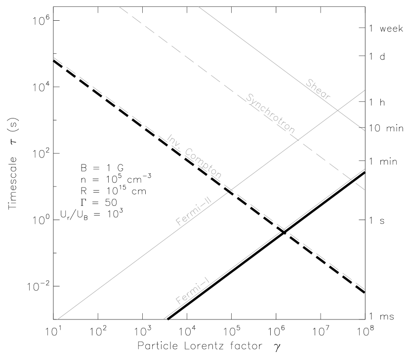
Figure 4: Calculated timescales in the comoving frame of the radiating plasma as a function of the particle Lorentz factor. Acceleration timescales (solid lines) are shown for the first-order Fermi acceleration (labelled Fermi-I) for electron, second-order acceleration (Fermi-II) for an electron in a hydrogen plasma, and shear acceleration, and losses (dashed lines) due to radiation due to synchrotron and IC; escape losses are too slow to appear in this Figure. The thick black lines show the fastest gain and loss timescales. Values for the magnetic field $B$, plasma number density $n$, bulk Lorentz factor $\Gamma$, and the ratio $U_{\rm rad}/U_{\rm mag}$ are given in the figure.

We have compared the various acceleration and loss timescales for various different physical environments by changing the following parameters: magnetic field intensity, matter density, size of the region, the jet Lorentz factor, and the ratio of radiation energy density to that of the magnetic field. In Fig. 4 the acceleration and loss timescales are shown for a set of parameters that correspond to the recent models of Ghisellini & Tavecchio (2008) and Begelman et al. (2008). The bold lines correspond to the fastest acceleration (marked with solid lines) and loss (dashed lines) timescales, and their crossing point corresponds to the Lorentz factor where gains and losses are equal – beyond this particles cool instead of accelerating. The most severe energy loss mechanism is the inverse Compton process, due to $U_{\rm rad}/U_{\rm mag}>1$. With the aforementioned assumptions, the particle escape process is orders of magnitude too slow to affect the radiating electrons significantly within timescales of minutes or hours.

The spatial scale affects the escape and shear acceleration timescales in the same way: both processes become more important for smaller sizes, and when considering minute- or even hour-scale variability in sources with $R\sim 10^{15}$ cm, both are negligible. It is possible, however, that if the particle scattering mean free path is significantly larger than the particle gyroradius, both processes begin to have noticeable effects.

The first-order process (including the effects of converter mechanism) accelerates electrons up to $\gamma\sim 10^{6}$ in just seconds, so it is fair to say that even in these short flares acceleration can be considered instantaneous. However, at the same time the second-order mechanism works on slower but still interesting timescales.

The plasma density directly affects only the second-order acceleration rate through the Alfvén-speed dependence: higher density leading to slower acceleration. Composition of the plasma has the same effect, because the presence of heavier ions decreases the Alfvén speed.

The expected rapid second-order acceleration process raises two important questions. Firstly, is the effect of stochastic acceleration seen in the observations? And, secondly, if it is not an important process, how do we explain this? For the first question, some recent observations of particle spectra with very hard power-law spectral indices ($\sigma<2$, for $N(\gamma)\propto\gamma^{-\sigma}$) suggest we may see it (Katarzyński et al., 2006; Böttcher et al., 2007).

The latter question, i.e., if we do not see stochastic acceleration even if the conditions seem perfect for it, suggests basically three plausible options.

Turning to the second question, an absence of stochastic acceleration would raise the following possibilities. Firstly, the acceleration model could be wrong. However, for the reasons given later in the discussion, we do not believe this to be the case and leave this option for other authors. Secondly, it is likely that we do not fully understand the plasma parameters such as composition and the magnetic field. Thirdly, the conditions are right, but there are other factors suppressing the acceleration or turning it off. This is also a realistic scenario, as we have very little knowledge of the nature and extent of the turbulence in the acceleration and radiating regions. A turbulence damping process could shut down this mechanism. This option is very plausible, because the process depends heavily on the turbulence in the acceleration regions, and very little is known about it. Furthermore, the stochastic acceleration in relativistic shocks and AGN-related conditions is still little studied. It is not unlikely that future studies will be able to set stricter limits for the extent (both spatial and energetic) of the process, making only a small region immediately behind the turbulence-creating shock front suitable for stochastic acceleration.

4.1 Absence of continuous acceleration

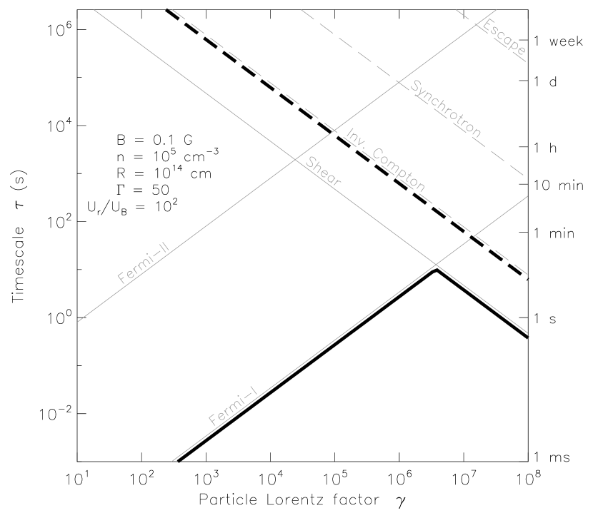
Figure 5: An example of parameter set which leads to a possible dominance of acceleration at all energies: low magnetic field and strong shear make the shear acceleration energise high-energy particles faster than the IC radiation decreases the energy.

It is interesting to note that with the assumption of high-velocity plasma streaming (whether as a continuous jet or an ejected plasma “blob”) within an external plasma, there always seems to be suitable conditions for very rapid particle acceleration. The acceleration can be “instantaneous” first-order acceleration – feeding the radiating region constantly with a power law of high-energy particles – or it can be a more gradual process, changing the energy distribution of the radiating particles on longer timescales.

When looking for a set of parameters that would yield dominating energy losses – corresponding to models with instantaneous acceleration to a power-law spectrum followed by only radiative cooling and other losses – we could not find any within limits typically considered physical for these sources: $B\in[10^{-3},1]$ G; $\Gamma\in[2,50]$; $n\in[1,10^{10}]$ cm^-3; $R\in[10^{10},10^{15}]$ cm; $U_{\rm rad}/U_{\rm mag}\in[10^{-3},10^{3}]$. Acceleration times within these limits were always shorter than the loss timescales in the lower energies up to electron Lorentz factors $\gamma\sim 10^{5-6}$. In fact, in some cases the “inverse” energy dependence of the shear acceleration led to domination of acceleration on all energies – an example of this is shown in Fig. 5. Although we don’t expect this to be a typical case in real sources (for reasons discussed earlier) it underlines the problem of getting only cooling without having acceleration at the same time.

4.2 Time delays

Interesting constraints on acceleration mechanisms arise from observations of a TeV flare of Markarian 501 on July 9th, 2005. Here the hard gamma-rays (2.7 TeV) were observed to lag behind the soft ones (190 GeV) by roughly four minutes. Similar “hard lags” have been observed earlier also in the X-ray domain (e.g., Brinkmann et al., 2005, for Markarian 401), but no definite explanation has been found yet. The “soft lags” – where lower-energy radiation peaks later than the higher-energy one – are easier to explain by high-energy radiating particle cooling and radiating on lower and lower frequencies, but, intuitively, these hard lags would require particles not cooled but heated or accelerated during the flare.

The observed delay has been proposed as being sue to the radiating blob accelerating during the flare by Bednarek & Wagner (2008), but even in their model the particles would only undergo cooling without any ongoing acceleration in or around the high-$\Gamma$ plasma flow. Mastichiadis & Moraitis (2008), however, showed that the observed features can be explained with a very simple and physically plausible modification, namely allowing the particles to accelerate gradually. In their model the acceleration time is of the order of hours and the electrons reach energies corresponding to $\gamma\sim 10^{6}$. The timescale may be too long for the first-order mechanism, but, interestingly, matches well to the stochastic acceleration timescale corresponding to their parameters.

Furthermore, similar slow energisation was quantitatively predicted by Virtanen & Vainio (2005), whose simulations of stochastic acceleration in relativistic shocks showed a gradual shift of the whole particle spectrum to higher energies as the particles were accelerated behind a shock front. Hadronic process could also be relevant within this model.

4.3 Generation of turbulence

Finally, one must also remember that as the accelerating particles need electromagnetic turbulence for scattering and energy gain, it is obvious that suitable turbulence either has to exist in the pre-shock plasma or be generated at the shock by the particles themselves. All models with instantaneous or constant first-order Fermi acceleration require the acceleration timescale to be significantly less than the flaring time, and the same limit is set also for the turbulence generation. Recent numerical work has addressed the problem of turbulence generation, and although the problem is still far from being solved, studies such as that by Reville et al. (2006), suggest that especially nonlinear turbulence generation by the particles themselves (found by Bell, 2004) could indeed be efficient enough to provide sufficient turbulence for fast acceleration.

5 Conclusions

We have estimated the timescales of different particle-acceleration mechanisms in the context of minute-scale TeV blazar flares. We have excluded both the neutron-based converter mechanism and shear acceleration from the dominating processes in these sources on observed timescales of the order of minutes. Furthermore, the first-order Fermi acceleration of protons is likely to be too slow to appear “instantaneous”. Instead, the accelerated proton distribution is expected to continue to be energised during the flare and could have special significance in hard-lag sources.

Various simultaneously active acceleration mechanisms working on different timescales suggest that in these sources one could expect to find slower, gradual energisation in addition to instantaneous – or a brief initial period of – acceleration. This speaks in favour of models with ongoing acceleration, instead of models with instantaneous injection of a fully-developed power-law spectrum which then only undergoes cooling. However, since many models that only include cooling can reproduce the observations, their results combined with timescale analysis could be helpful in studying the source parameters.

We emphasise that the current model is very simplified. The results neglect, in particular, the Klein-Nishina effects in the energy losses of the highest-$\gamma$ particles. Also, the magnetic field is assumed to be constant throughout the flare, although generation of turbulence and the subsequent increase in the magnetic field strength can decrease the synchrotron loss timescales significantly (Schlickeiser & Lerche, 2007). Furthermore, because the acceleration efficiency depends on the scattering mean free path, for different scattering models the acceleration timescales could also change. Furthermore, other omitted turbulence-affecting effects can decrease the acceleration timescales, for example by increasing the acceleration efficiency. An example is the case of turbulence transmission leading to an increased scattering-centre compression ratio (see Vainio et al., 2003; 2005, and Tammi & Vainio 2006), and enhanced first-order acceleration at the shock in conditions similar to AGN or microquasar jets (Tammi, 2008). However, even in its current state, especially in the lower-energy part of the particle spectrum ($\gamma\lesssim 10^{4}$) the present analysis still provides a useful tool for estimating the source properties.

Finally, we note that since the acceleration efficiency depends on the scattering mean free path differently for each of the processes, detailed modelling could provide additional tests when we learn more about the intrinsic properties of the plasma and turbulence in these sources.

References

- Aharonian et al. (2007) Aharonian, F. et al. 2007, ApJL, 664, L71
- Albert et al. (2007) Albert, J. et al. 2007, ApJL, 669, 862
- Bednarek & Wagner (2008) Bednarek, W. & Wagner, R.M. 2008, A&A, 486, 679
- Begelman et al. (2008) Begelman, M. C., Fabian, A. & Rees, M.J. 2008, MNRAS, 384, L19
- Bell (2004) Bell, A. R. 2004, MNRAS, 353, 550
- Böttcher et al. (2007) Böttcher, M., Dermer, C. D. & Finke, J. D. 2008, ApJL, 679, 9
- Brinkmann et al. (2005) Brinkmann, W., Papadakis, I. E., Raeth, C., Mimica, P. & Haberl, F. 2005, A&A, 443, 397
- Celotti & Ghisellini (2008) Celotti, A. & Ghisellini, G. 2008, MNRAS, 385, 283
- Derishev et al. (2003) Derishev, E. V., Aharonian, F. A., Kocharovsky, V. V. & Kocharovsky, Vl. V. 2003, Phys. Rev. D, 68, 3003
- Ghisellini & Tavecchio (2008) Ghisellini, G. & Tavecchio, F. 2008, MNRAS, 386, L28
- Katarzyński et al. (2006) Katarzyński, K., Ghisellini, G., Mastichiadis, A., Tavecchio, F. & Maraschi, L. 2006, A&A, 453, 47
- Longair (1994) Longair, M.S. 1994, High Energy Astrophysics, vol. 2, Cambridge University Press, Cambridge, MA, USA, 1994
- Mastichiadis & Moraitis (2008) Mastichiadis, A. & Moraitis, K. 2008, A&A, 491, L37
- Reville et al. (2006) Reville, B., Kirk, J.G. & Duffy, P. 2006, Plasma Phys. Control. Fusion 48, 1741
- Rieger & Duffy (2004) Rieger, F. & Duffy, P. 2004, ApJ, 617, 155
- Rieger et al. (2007) Rieger, F., Bosch-Ramon, V. & Duffy, P. 2007, Ap&SS, 309, 119
- Schlickeiser & Lerche (2007) Schlickeiser, R. & Lerche, I. 2007, A&A, 476, 1
- Stern (2008) Stern, B. E. 2003, MNRAS, 345, 590
- Stern & Poutanen (2008) Stern, B. E. & Poutanen, J. 2008, MNRAS, 383, 1695
- Tammi (2008) Tammi, J. 2008, IJMPD, 17, 1811
- Tammi & Vainio (2006) Tammi, J. & Vainio, R. 2006, A&A 460, 23
- Vainio et al. (2003) Vainio, R., Virtanen, J.J.P. & Schlickeiser, R. 2003, A&A 409, 821
- Vainio et al. (2005) Vainio, R., Virtanen, J.J.P. & Schlickeiser, R. 2005, A&A 431, 7
- Virtanen & Vainio (2005) Virtanen, J.J.P. & Vainio, R. 2005, ApJ 621, 313