Faster Approximate String Matching for Short Patterns

Abstract

We study the classical approximate string matching problem, that is, given strings $P$ and $Q$ and an error threshold $k$, find all ending positions of substrings of $Q$ whose edit distance to $P$ is at most $k$. Let $P$ and $Q$ have lengths $m$ and $n$, respectively. On a standard unit-cost word RAM with word size $w\geq\log n$ we present an algorithm using time

$$O\left(nk\cdot\min\left(\frac{\log^{2}m}{\log n},\frac{\log^{2}m\log w}{w}\right)+n\right)$$

When $P$ is short, namely, $m=2^{o(\sqrt{\log n})}$ or $m=2^{o(\sqrt{w/\log w})}$ this improves the previously best known time bounds for the problem. The result is achieved using a novel implementation of the Landau-Vishkin algorithm based on tabulation and word-level parallelism.

1 Introduction

Given strings $P$ and $Q$ and an error threshold $k$, the approximate string matching problem is to report all ending positions of substrings of $Q$ whose edit distance to $P$ is at most $k$. The edit distance between two strings is the minimum number of insertions, deletions, and substitutions needed to convert one string to the other. Approximate string matching is a classical and well-studied problem in combinatorial pattern matching with a wide range of applications in areas such as bioinfomatics, network traffic analysis, and information retrieval.

Let $m$ and $n$ be the lengths of $P$ and $Q$, respectively, and assume without loss of generality that $k<m\leq n$. The classic textbook solution to the problem, due to Sellers [27], fills in an $(m+1)\times(n+1)$ distance matrix $C$ such that $C_{i,j}$ is the smallest edit distance between the $i$th prefix of $P$ and a substring of $Q$ ending at position $j$. Using dynamic programming, we can compute each entry in $C$ in constant time leading to an algorithm using $O(nm)$ time.

Several improvements of this algorithm are known. Masek and Paterson [22] showed how to compactly encode and tabulate solutions to small submatrices of the distance matrix. We can then traverse multiple entries in the table in constant time leading to an algorithm using $O(nm/\log^{2}n+n)$ time. This bound assumes constant size alphabets. For general alphabets, the best bound is $O(nm(\log\log n)^{2}/\log^{2}n+n)$ [9]. This tabulation technique is often referred to as the Four Russian technique after Arlazarov et al. [4] who introduced it for boolean matrix multiplication. Alternatively, several algorithms using the arithmetic and logical operations of the word RAM to simulate the dynamic program have been suggested [5, 32, 31, 6, 24, 18]. This technique is often referred to as word-level parallelism or bit-parallelism. The best known bound is due to Myers [24] who gave an algorithm using $O(nm/w+n)$ time. In terms of $n$ and $m$ alone, these are the best known bounds for approximate string matching. However, if we take into account the error threshold $k$, several faster algorithms are known [29, 28, 23, 13, 20, 14, 26, 10]. These algorithms exploit properties of the diagonals of the distance matrix $C$ and are therefore often called diagonal transition algorithms. The best known bound is due to Landau and Vishkin [20] who gave an $O(nk)$ algorithm. Compared to the algorithms by Masek and Paterson and by Myers, the Landau-Vishkin algorithm (abbreviated LV-algorithm) is faster for most values of $k$, namely, whenever $k=o(m/\log^{2}n)$ or $k=o(m/w)$. For $k=O(m^{1/4})$, Cole and Hariharan showed that it is even possible to solve approximate string matching in $O(n)$ time. Their algorithm “filters” out all but a small set of positions in $Q$ which are then checked using the LV-algorithm.

All of the above bounds are valid on a unit-cost RAM with $w$-bit words and a standard instruction set including arithmetic operations, bitwise boolean operations, and shifts. Each word is capable of holding a character of $Q$ and hence $w\geq\log n$. The space complexity is the number of words used by the algorithm, not counting the input which is assumed to be read-only. For simplicity, we assume that suffix trees can be constructed in linear time which is true for any polynomially sized alphabet [12]. This assumption is also needed to achieve the $O(nk)$ bound of the Landau-Vishkin algorithm [20]. Without it, additional time for sorting the alphabet is required [12]. All the results presented here assume the same model.

1.1 Results

We present a new algorithm for approximate string matching achieving the following bounds.

Theorem 1

Approximate string matching for strings $P$ and $Q$ of length $m$ and $n$, respectively, with error threshold $k$ can be solved

• in time $O(nk\cdot\frac{\log^{2}m}{\log n}+n)$ and space $O(n^{\epsilon}+m)$, for any constant $\epsilon>0$, and

• in time $O(nk\cdot\frac{\log^{2}m\log w}{w}+n)$ and space $O(m)$.

When $P$ is short, namely, $m=2^{o(\sqrt{\log n})}$ or $m=2^{o(\sqrt{w/\log w})}$, this improves the $O(nk)$ time bound and places a new upper bound on approximate string matching. For many practically relevant combinations of $n$, $m$ and $k$ this significantly improves the previous results. For instance, when $m$ is polylogarithmic in $n$, that is, $m=O(\log^{c}n)$ for a constant $c>0$, Theorem 1(i) gives us an algorithm using time $O(nk\cdot\frac{(\log\log n)^{2}}{\log n}+n)$. This is almost a logarithmic speed-up of $O(\frac{\log n}{(\log\log n)^{2}})$ over the $O(nk)$ bound. Note that the exponent $c$ only affects the constants in asymptotic time bound. For larger $m$, the speed-up smoothly decreases until $m=2^{\Theta(\sqrt{\log n})}$, where we arrive at the $O(nk)$ bound.

The algorithm for Theorem 1(i) tabulates certain functions on $\epsilon\log n$ bits which lead to the additional $O(2^{\epsilon\log n})=O(n^{\epsilon})$ space. The algorithm for Theorem 1(ii) instead uses word-level parallelism and therefore avoids the additional space for lookup tables. Furthermore, for $w=O(\log n)$, Theorem 1(ii) gives us an algorithm using time $O(nk\cdot\frac{\log^{2}m\log\log n}{\log n}+n)$. This is a factor $O(\log\log n)$ slower than Theorem 1(i). However, the bound increases with $w$ and whenever $w\log w=\omega(\log n)$, Theorem 1(i) is the best time bound.

1.2 Techniques

The key idea to obtain our bounds is a novel implementation of the LV-algorithm that reduces approximate string matching to $2$ operations on a compact encoding of the “state” of the LV-algorithm. We show how to implement these operations using tabulation for Theorem 1(i) or word-level parallelism for Theorem 1(ii). As discussed above, several improvements of Sellers classical dynamic programming algorithm [27] based on tabulation and word-level parallelism are known. However, for diagonal transition algorithms no similar tabulation or word-level parallelism improvements exists. Achieving such a result is also mentioned as an open problem in a recent survey by Navarro [25, p.61]. The main problem is the complicated dependencies in the computation of the LV-algorithm. In particular, in each step of the LV-algorithm we map entries in the distance matrix to nodes in the suffix tree, answer a nearest common ancestor query, and map information associated with the resulting node back to an entry in the distance matrix. To efficiently compute this information in parallel, we introduce several new techniques. These techniques differ significantly from the techniques used to speed-up Sellers algorithm, and we believe that some of them might be of independent interest. For example, we give a new algorithm to efficiently evaluate a compact representation of a function on several inputs in parallel. We also show how to use a recent distributed nearest common ancestor data structure to efficiently answer multiple nearest common ancestor queries in parallel.

The results presented in this paper are mainly of theoretical interest. However, we believe that some of the ideas have practical relevance. For instance, it is often reported that the nearest common ancestor computations make the LV-algorithm unsuited for practical purposes [25]. With our new algorithm, we can compute several of these in parallel and thus target this bottleneck.

1.3 Outline

The paper is organized as follows. In Section 2 we review the basic concepts and the LV-algorithm. In Section 3 we introduce the packed representation and the key operations needed to manipulate it. In Section 4.2 we reduce approximate string matching to two operations on the packed representation. Finally, in Sections 5 and Section 6 we present our tabulation based algorithm and word-level parallel algorithm for these operations.

2 Preliminaries

We review the necessary concepts and the basic algorithms for approximate string matching. We will use these as a starting point for our own algorithms.

2.1 Strings, Trees, and Suffix Trees

Let $S$ be a string of length $|S|$ on an alphabet $\Sigma$. The character at position $i$ in $S$ is denoted by $S[i]$, and the substring from position $i$ to $j$ is denoted by $S[i,j]$. The substrings $S[1,j]$ and $S[i,|S|]$ are the prefixes and suffixes of $S$, respectively. The longest common prefix of two strings is the common prefix of maximum length.

Let $T$ be a rooted tree with $|T|$ nodes. A node $v$ in $T$ is an ancestor of a node $w$ if $v$ is on the path from the root to $w$ (including $v$ itself). A node $z$ is a common ancestor of nodes $v$ and $w$ if $z$ is an ancestor of both. The nearest common ancestor of $v$ and $w$, denoted $\mathrm{nca}(v,w)$, is the common ancestor of $v$ and $w$ of maximum depth in $T$. With linear space and preprocessing time, we can answer $\mathrm{nca}$ queries in constant time [17] (see also [8, 2]).

The suffix tree for $S$, denoted $T_{S}$, is the compacted trie storing all suffixes of $S$ [15]. Each edge $e$ in $T_{S}$ is associated with a substring of $S$, called the edge-label of $e$. The concatenation of edge-labels on a path from the root to a node $v$ is called the path-label of $v$. The string-depth of $v$, denoted $\mathrm{strdepth}(v)$, is the length of the path-label of $v$. The $i$th suffix of $S$ is represented by the unique leaf in $T_{S}$ whose path-label is $S[i,|S|]$, and we denote this leaf by $\mathrm{leaf}(i)$. The suffix tree uses linear space and can be constructed in linear time for polynomially sized alphabets [12].

A useful property of suffix trees is that for any two leaves $\mathrm{leaf}(i)$ and $\mathrm{leaf}(j)$, the path label of the node $\mathrm{nca}(\mathrm{leaf}(i),\mathrm{leaf}(j))$ is longest common prefix of the suffixes $S[i,|S|]$ and $S[j,|S|]$ [15]. Hence, if we construct a nearest common ancestor data structure for $T_{S}$ and compute the string depth for each node in $T_{S}$, we can compute the length of the longest common prefix of any two suffixes in constant time.

For a set of strings $S_{1},\ldots,S_{l}$ it is straightforward to construct a suffix tree $T_{S_{1},\ldots,S_{l}}$ storing all suffixes of each string in $S_{1},\ldots,S_{l}$ [15]. A suffix tree of more than one string is often called a generalized suffix tree [15]. The space for $T_{S_{1},\ldots,S_{l}}$ is linear in the total length of the strings.

2.2 Algorithms for Approximate String Matching

Recall that $|P|=m$ and $|Q|=n$ and $k$ is the error threshold. The algorithm by Sellers [27] fills in a $(m+1)\times(n+1)$ matrix $C$ according to the following rules:

$$C_{i,0} =i\qquad 0\leq i\leq m$$ (1)

$$C_{0,j} =0\qquad 0\leq j\leq n$$

$$C_{i,j} =\min(C_{i-1,j-1}+\delta(p_{i},t_{j}),C_{i-1,j}+1,C_{i,j-1}+1)\qquad 1\leq i\leq m,1\leq j\leq n$$

For any pair of characters $a$ and $b$, $\delta(a,b)=0$ if $a=b$ and $1$ otherwise. An example of a matrix is shown in Figure 1. Note that the above rules are the same as for the classical dynamic program for the well-known edit distance problem [30], except for the boundary condition $C_{0,j}=0$. The entry $C_{i,j}$ is the minimum edit distance between $P[1,i]$ and any substring of $Q$ ending at position $j$. Hence, there is a match of $P$ with a most $k$ edits that ends at $Q[j]$ iff $C_{m,j}\leq k$. Using dynamic programming, we can compute each entry in constant time leading to an $O(nm)$ solution.

Landau and Vishkin [20] presented a faster algorithm to compute essentially the same information as in (1). We will refer to this algorithm as the LV-algorithm in the rest of the paper. Define the diagonal $d$ of $C$ to be the set of entries $C_{i,j}$ such that $j-i=d$. Given a diagonal $d$ and integer $e$, define the diagonal position $L_{d,e}$ to be the maximum $i$ such that $C_{i,j}=e$ and $C_{i,j}$ is on diagonal $d$. There is a match of $P$ with a most $k$ edits that ends at $Q[d+m]$ iff $L_{d,e}=m$, for some $e\leq k$. Let $\mathrm{lcp}(i,j)$ denote the length of the longest common prefix of $P[i,m]$ and $Q[j,n]$. Using the clever observation that entries in a diagonal are non-decreasing in the downwards direction, Landau and Vishkin gave the following rules to compute $L_{d,e}$.

$$L_{d,-1} =L_{n+1,e}=-1\qquad\text{for $e\in\{-1,\ldots,k\}$ and $d\in\{0,\ldots,n\}$}$$ (2a)

$$L_{d,|d|-2} =|d|-2\qquad\text{for $d\in\{-(k+1),\ldots,-1\}$}$$ (2b)

$$L_{d,|d|-1} =|d|-1\qquad\text{for $d\in\{-(k+1),\ldots,-1\}$}$$ (2c)

$$L_{d,e} =z+\mathrm{lcp}(z+1,d+z+1)$$ (2d)

$$\text{where }z =\min(m,\max(L_{d,e-1}+1,L_{d-1,e-1},L_{d+1,e-1}+1))$$ (2e)

Lines (2a), (2b), and (2c) are boundary conditions. Lines (2d) and (2e) determine $L_{d,e}$ from $L_{d,e-1}$, $L_{d-1,e-1}$, $L_{d+1,e-1}$, and the length of the longest common prefix of $P[z+1,m]$ and $Q[d+z+1,n]$. Hence, we can compute a matrix $L$ of diagonal positions by iteratively computing the sets of diagonal positions $L_{-1},L_{0},\ldots,L_{k}$, where $L_{e}$ denotes the set of entries in $L$ with error $e$. Since we can compute $\mathrm{lcp}$ queries in constant time using a nearest common ancestor data structure, the total time to fill in the $O(nk)$ entries of $L$ is $O(nk)$. Each set of diagonal positions and the suffix tree require $O(n)$ space. However, we can always divide $Q$ into overlapping substrings of length $2m-2k$ with adjacent substrings overlapping in $m+k-1$ characters. A substring matching $P$ with at most $k$ errors must have a length in the range $[m-k,m+k]$ and therefore all matches are completely contained within a substring. Applying the LV-algorithm to each of the substrings independently solves approximate string matching in time $O(n/m\cdot mk)=O(nk)$ as before, however, now the space is only $O(m)$.

		s	u	r	g	e	r	y
	0	0	0	0	0	0	0	0
s	1	0	1	1	1	1	1	1
u	2	1	0	1	2	2	2	2
r	3	2	1	0	1	2	2	3
v	4	3	2	1	1	2	3	3
e	5	4	3	2	2	1	2	3
y	6	5	4	3	3	2	2	2

Figure 1: The dynamic programming matrix $C$ for $P=\texttt{survey}$ and $Q=\texttt{surgery}$ (adapted from Navarro [25]). $P$ matches $Q$ with edit distance $2$ at positions $5$, $6$, and $7$. In diagonal $1$, the maximum rows indices containing $0$, $1$, and $2$ are $0$, $3$, and $6$, respectively. Hence, $L_{1,0}=0$, $L_{1,1}=3$, and $L_{1,2}=6$.

3 Manipulating Bits

In this section we introduce the necessary notation and key primitives for manipulating bit strings.

Let $x=b_{f}\ldots b_{1}$ be a bit string consisting of bits $b_{1},\ldots,b_{f}$ numbered from right-to-left. The length of $x$, denoted $|x|$, is $f$. We use exponentiation for bit repetition, i.e., $0^{3}1=0001$ and $\cdot$ for concatenation, i.e., $001\cdot 100=001100$. In addition to the arithmetic operators $+$, $-$, and $\times$ we have the operators $\>\&\>$, $\mid$, and $\oplus$ denoting bit-wise ‘and’, ‘or’, and ‘exclusive-or’, respectively. Moreover, $\overline{x}$ is the bit-wise ‘not’ of $x$ and $x\ll j$ and $x\gg j$ denote standard left and right shift by $j$ positions. The word RAM supports all of these above operators for bit strings stored in single words in unit time [16]. Note that for bit strings of length $O(w)$ (recall that $w$ is the number of bits in a word) we can still simulate these instructions in constant time.

We will use the following nearest common ancestor data structure based on bit string labels in our algorithms.

Theorem 2 (Alstrup et al. [2])

There is a linear time algorithm that labels the $t$ nodes of a tree $T$ with bit strings of length $O(\log t)$ bits such that from the labels of nodes $v$ and $w$ in $T$ alone, one can compute the label of $\mathrm{nca}(v,w)$ in constant time.

For our purposes, we will slightly modify the above labeling scheme such that all labels have the same length $f=O(\log t)$. This is straightforward to do and we will present one way to do it later in Section 6.4.1. Let $\mathrm{label}(v)$ denote the label of a node $v$ in $T$. The label nearest common ancestor, denoted $\mathrm{lnca}$, is the function given by $\mathrm{lnca}(\mathrm{label}(v),\mathrm{label}(w))=\mathrm{label}(\mathrm{nca}(v,w))$ for any pair of labels $\mathrm{label}(v)$ and $\mathrm{label}(w)$ of nodes $v$ and $w$ in $T$. Thus, $\mathrm{lnca}$ maps two bit strings of length $f$ to a single bit string of length $f$.

3.1 Packed Sequences

We often interpret bit strings as sequences of smaller bit strings and integers. For a sequence $x_{1},\ldots,x_{r}$ of bit strings of length $f$, define the $f$-packed sequence $X=\langle{x_{1},\ldots,x_{r}}\rangle$ to be the bit string

$$0\cdot x_{r}\cdot 0\cdot x_{r-1}\cdots 0\cdot x_{2}\cdot 0\cdot x_{1}$$

Each substring $0\cdot x_{i}$, $1\leq i\leq r$, is a field. The leftmost bit of a field is the test bit and the remaining $f$ bits, denoted $X\langle{i}\rangle=x_{i}$, is the entry. The length of a $f$-packed sequence is the number of fields in it. Note that a $f$-packed sequence of length $r$ is represented by a bit string of length $r(f+1)$. If $x_{1},\ldots,x_{r}$ is a sequence of $f$-bit integers, $\langle{x_{1},\ldots,x_{r}}\rangle$ is interpreted as $\langle{\mathrm{bin}(x_{1}),\ldots,\mathrm{bin}(x_{r})}\rangle$, where $\mathrm{bin}(x)$ is the binary encoding of $x$. We represent packed sequences compactly in words by storing $s=\left\lfloor{w/(f+1)}\right\rfloor$ fields per word. For our purposes, we will always assume that fields are capable of storing the total number of fields in the packed sequence, that is, $f\geq\log r$. Given another $f$-packed sequence $Y=\langle{y_{1},\ldots,y_{r}}\rangle$, the zip of $X$ and $Y$, denoted $X\ddagger Y$, is the $2f$-packed sequence $\langle{(x_{1},y_{1}),\ldots,(x_{r},y_{r})}\rangle$ (the tuple notation $(x_{i},y_{i})$ denotes the bit string $x_{i}\cdot y_{i}$). Packed sequence representations are well-known within sorting and data structures (see, e.g., the survey by Hagerup [16]). In the following we review some basic operations on them.

Let $X=\langle{x_{1},\ldots,x_{s}}\rangle$ and $Y=\langle{y_{1},\ldots,y_{s}}\rangle$ be $f$-packed sequences of length $s=\left\lfloor{w/(f+1)}\right\rfloor$. Hence, $X$ and $Y$ can each be stored in a single word of $w$ bits. We consider the general case of longer packed sequences later. Some of our operations require precomputed constants depending on $s$ and $f$, which we assume are available (e.g., computed at “compile-time”). If this is not the case, we can always precompute these constants in time $\log^{O(1)}w$ which is neglible.

Elementwise arithmetic operations (modulo $2^{f}$) and bit-wise operations are straightforward to implement in $O(1)$ time using the built-in operations. For example, to compute $\langle{x_{1}+y_{1}\mod 2^{f},\ldots,x_{s}+y_{s}\mod 2^{f}}\rangle$, we add $X$ and $Y$ and clear the test bits by $\>\&\>$’ing with the constant $I_{s,f}=(10^{f})^{s}$ ($I_{s,f}$ consists of $1$’s at all test bit positions). The test bit positions ensures that no overflow bits from the addition can affect neighbouring entries.

The compare of $X$ and $Y$ with respect to an operator $\bowtie\>\in\{=,\neq,\geq,\leq\}$, is the bit string $C$, where all entries are $0$ and the $i$th test bit is $1$ iff $x_{i}\bowtie y_{i}$. For the $\geq$ operator, we compute the compare as follows. Set the test bits of $X$ by $\mid$’ing with $I_{s,f}$, then subtract $Y$, and mask out the test bits by $\>\&\>$’ing with $I_{s,f}$. It is straightforward to show that the $i$th test bit in the result “survives” the subtraction iff $x_{i}\geq y_{i}$. The entire operation takes $O(1)$ time. We can similarly compute the compare with respect to the other operators ($=$, $\neq$, and $\leq$) in constant time.

Given a sequence of test bits $t_{1},\ldots,t_{s}$ stored at test bit position in a bit string $T$, i.e., $T=t_{s}\cdot 0^{f}\ldots t_{1}0^{f}$, the extract of $X$ with respect to $T$, is the $f$-packed sequence $E$ given by

$$E\langle{i}\rangle=\begin{cases}x_{i}&\text{if $t_{i}=1$},\\ 0&\text{otherwise}.\end{cases}$$

We compute the extract operation as follows. First, copy each test bit to all positions in their field by subtracting $(I_{s,f}\gg f)$ from $T$. Then, $\&$ the result with $X$. Again, the operation takes $O(1)$ time. We can combine the compare and extract operation to compute more complicated operations. For instance, to compute the elementwise maximum $M=\langle{\max(x_{1},y_{1}),\ldots,\max(x_{s},y_{s})}\rangle$, compare $X$ and $Y$ with respect to $\geq$ and let $T$ be the result. Extract from $X$ with respect to $T$, the packed sequence $M_{X}$ containing all entries in $X$ that are greater than or equal to the corresponding entry in $Y$. Also, extract from $Y$ with respect to $\overline{T}\>\&\>I_{r,f}$, the packed sequence $M_{Y}$ containing all entries in $Y$ that are greater than or equal to the corresponding entry in $X$. Finally, combine $M_{X}$ and $M_{Y}$ into $M$ by $\mid$’ing them.

Let $z$ be a $f$-bit integer. The rank of $z$ in $X$, denoted by $\mathrm{rank}(X,z)$, is the number of entries in $X$ smaller than or equal to $z$. We can compute $\mathrm{rank}(X,z)$ in constant time as follows. First, replicate $z$ to all fields in a words by computing $Z=z\times 1(0^{f}1)^{s}=\langle{z,\ldots,z}\rangle$. Then, compare $X$ and $Z$ with respect to $\geq$ and store the result in a word $C$. The number of $1$ bits in $C$ is $\mathrm{rank}(X,z)$. To count these, we compute the suffix sum of the test bits by multiplying $C$ with $(0^{f}1)^{s}$. This produces a word $P$ such that $P\langle{i}\rangle$ is number of test bits in the rightmost $i$ field of $C$. Finally, we extract $P\langle{s}\rangle$ as the result. Note that the condition $f\geq\log r$ is needed here.

All of the above $O(1)$ time algorithms, except $\mathrm{rank}$, are straightforward to generalize efficiently to longer $f$-packed sequences. For $f$-packed sequences of length $r>s$ the time becomes $O(r/s+1)=O(rf/w+1)$.

We will also need more sophisticated packed sequence operations. First, define a $f$-packed function of length $u$ to be a $2f$-packed sequence $G=\langle{(z_{1},g(z_{1})),\ldots,(z_{u},g(z_{u}))}\rangle$, where $z_{1}<\cdots<z_{u}$ and $g$ is any function mapping a bit string of length $f$ to a bit string of length $f$. The domain of $G$, denoted $\mathrm{dom}(G)$, is the sequence $\langle{z_{1},\ldots,z_{u}}\rangle$. Let $X=\langle{x_{1},\ldots,x_{r}}\rangle$ and $Y=\langle{y_{1},\ldots,y_{r}}\rangle$ be $f$-packed sequences and let $G$ be a $f$-packed function such that each entry in $X$ appears in $\mathrm{dom}(G)$. Define the following operations.

• Return the $f$-packed sequence $\langle{g(x_{1}),\ldots,g(x_{r})}\rangle$.

• Return the $f$-packed sequence $\langle{\mathrm{lnca}(x_{1},y_{1}),\ldots,\mathrm{lnca}(x_{r},y_{r})}\rangle$.

In other words, the Map operation applies $g$ to each entry in $X$ and Lnca is the elementwise version of the $\mathrm{lnca}$ operation. We believe that an algorithm for these operations might be of independent interest in other applications. In particular, the Map operation appears to be a very useful primitive for algorithms using packed sequences. Before presenting our algorithms for Map and Lnca, we show how they can be used to implement the LV-algorithm.

4 From Landau-Vishkin to Mapping and Label Nearest Common Ancestor

In this section we give an implementation of the LV-algorithm based on the Map and Lnca operations. Let $P$ and $\widehat{Q}$ be strings of length $m$ and $2m-2k$ and $k$ be an error threshold. Recall from Section 2 that an algorithm for this case immediately generalizes to find approximate matches in longer strings. We preprocess $P$ and $\widehat{Q}$ and then use the constructed data structures to efficiently implement the LV-algorithm.

4.1 Preprocessing

We compute the following information. Let $r=O(m)$ be the number of diagonals in the LV-algorithm on $P$ and $\widehat{Q}$.

• The (generalized) suffix tree, $T_{P,\widehat{Q}}$, of $P$ and $\widehat{Q}$ containing $O(m)$ nodes and leaves. The leaf representing suffix $i$ in $P$ is denoted $\mathrm{leaf}(P,i)$, and the leaf representing suffix $j$ in $\widehat{Q}$ is denoted $\mathrm{leaf}(\widehat{Q},j)$.

• Nearest common ancestor labels for the nodes in $T_{P,\widehat{Q}}$ according to Theorem 2. Hence, the maximum length of labels is $f=O(\log m)$. We denote the label for a node $v$ by $\mathrm{label}(v)$.

• The $f$-packed functions $N_{P}$, $N_{\widehat{Q}}$, and $D$, representing the functions given by $n_{P}(i)=\mathrm{label}(\mathrm{leaf}(P,i))$, for $i\in\{1,\ldots,m\}$, $n_{\widehat{Q}}(j)=\mathrm{label}(\mathrm{leaf}(\widehat{Q},j))$, for $j\in\{1,\ldots,2m-2k\}$, and $d(\mathrm{label}(v))=\mathrm{strdepth}(v)$, for any node $v$ in $T_{P,\widehat{Q}}$.

• The $f$-packed sequences $1_{r,f}$ and $M_{r,f}$ consisting of $r$ copies of $1$ and $m$, respectively, and the $f$-packed sequence $J_{r,f}=\langle{1,2,\ldots,r}\rangle$.

Since $r=O(m)$, the space and preprocessing time for all of the above information is $O(m)$.

4.2 A Packed Landau-Vishkin Algorithm

Recall that the LV-algorithm iteratively computes the sets of diagonal positions $L_{-1},\ldots,L_{k}$, where $L_{e}$ is the set of entries in $L$ with error $e$. To implement the algorithm we represent each of the sets of diagonal positions as $f$-packed sequences of length $r$. We construct $L_{-1}$ by inserting each field in constant time according to (2). After computing $L_{k}$, we inspect each field in constant time and report any matches. These steps take $O(r)=O(m)$ time in total. We show how to compute the remaining sets of diagonal positions. Given $L_{e-1}$, $e\in\{0,\ldots,k\}$, we compute $L_{e}$ as follows. First, fill in the $O(1)$ boundary fields according to (2a), (2b), and (2c). Then, compute the remaining fields using the following $4$ steps.

Step 1: Compute Maximum Diagonal Positions

Compute the $f$-packed sequence $Z$ given by

$$Z\langle{d}\rangle:=\min\left(m,\max(L_{e-1}\langle{d}\rangle+1,L_{e-1}\langle{d-1}\rangle,L_{e-1}\langle{d+1}\rangle+1)\right).$$

Thus, $Z$ corresponds to the “$z$” part in (2e). We compute $Z$ efficiently as follows. First, construct the packed sequences $Z_{1}\langle{d}\rangle:=L_{e-1}\langle{d}\rangle+1$, $Z_{2}\langle{d}\rangle:=L_{e-1}\langle{d-1}\rangle$, and $Z_{3}\langle{d}\rangle:=L_{e-1}\langle{d+1}\rangle+1$ by shifting and adding $1_{r,f}$. Then, compute the elementwise maximum of $Z_{1}$, $Z_{2}$, and $Z_{3}$, and finally, the elementwise minimum with $M_{r,f}$.

Step 2: Translate to Suffixes

Compute the $f$-packed sequences $Z_{P}$ and $Z_{\widehat{Q}}$ given by

$$Z_{P}\langle{d}\rangle :=Z\langle{d}\rangle+1,$$

$$Z_{\widehat{Q}}\langle{d}\rangle :=Z\langle{d}\rangle+d+m.$$

Hence, $Z_{P}\langle{d}\rangle$ and $Z_{\widehat{Q}}\langle{d}\rangle$ contains the inputs to the $\mathrm{lcp}$ part in (2d). We can compute $Z_{P}$ by adding $1_{r,f}$ to $Z$ and $Z_{\widehat{Q}}$ by adding $J_{r,f}$ and $M_{r,f}$ to $Z$.

Step 3: Compute Longest Common Prefixes

Compute the $f$-packed sequence $\mathrm{LCP}$ given by

$$\mathrm{LCP}:=\textsc{Map}(D,\textsc{Lnca}(\textsc{Map}(N_{P},Z_{P}),\textsc{Map}(N_{\widehat{Q}},Z_{\widehat{Q}}))).$$

This corresponds to the computation of $\mathrm{lcp}$ in (2d).

Step 4: Update State

Finally, compute the new sequence $L_{e}$ of diagonal positions as

$$L_{e}\langle{d}\rangle=Z\langle{d}\rangle+\mathrm{LCP}\langle{d}\rangle.$$

This corresponds to the $+$ in (2d).

Steps $1$, $2$, and $4$ takes $O(rf/w+1)=O(m\log m/w+1)$ time. Note that a set of diagonal positions of LV-algorithm requires $O(m\log m)$ bits to be represented. Hence, to simply output a set of diagonal positions we must spend at least $\Omega(m\log m/w)$ time.

We parameterize the complexity for approximate string matching in terms of the complexity for the Lnca and Map operations.

Lemma 1

Let $P$ and $Q$ be strings of length $m$ and $n$, respectively, and let $k$ be an error threshold. Given a data structure using $s$ space and $p$ preprocessing time that supports Map and Lnca in time $q$ on $O(\log m)$-packed sequences of length $O(m)$, we can solve approximate string matching in time $O\left(\frac{nk}{m}\cdot q+\frac{nk\log m}{w}+p+n\right)$ and space $O(s+m)$.

Proof. We consider two cases depending on $n$. First, suppose that $n\leq 2m-2k$. Then, all of the packed sequences in the algorithm have length $O(m)$. Hence, we can use the data structure for Map and Lnca directly to implement step $3$ in time $q$. Since steps $1$, $2$, and $4$ use time $O(rf/w+1)=O(m\log m/w+1)$, we can compute all of the $k+1$ state transitions in time $O(k(q+\frac{m\log m}{w})+m)$. With additional time and space for preprocessing and using the fact that $n/m=O(1)$, the result follows. If $n>2m-2k$, we apply the algorithm to $O(n/m)$ substrings of length $2m-2k$ as described in Section 2. Since the computation for each of the substrings is independent, we can reuse space to get $O(p+m)$ space in total. The total time is

$$O\left(\frac{n}{m}\cdot k\cdot\left(q+\frac{m\log m}{w}\right)+p+n\right)=O\left(\frac{nk}{m}\cdot q+\frac{nk\log m}{w}+p+n\right).$$

$\Box$

5 Implementing Lnca and Map

In this and the following section we show how to implement the Lnca and Map operation efficiently.

For simplicity in the description of our algorithms, we will initially assume that our word RAM model supports a constant number of non-standard instructions. Specifically, in addition to the standard constant time instructions on words, e.g., arithmetic and bitwise logical instructions, we will allow a few special constant time instructions (the non-standard ones) defined by us. As with standard instructions, a non-standard instruction take $O(1)$ operand words and return $O(1)$ result words. We will subsequently implement the non-standard instructions using either tabulation or word-level parallelism. These two approaches lead to the two parts of Theorem 1. We emphasize that the main result in Theorem 1 only uses standard instructions.

To implement Lnca, we will simply assume that Lnca is itself available as a non-standard instruction. Specifically, given two $f$-packed sequences $X$ and $Y$ of length $s=\left\lfloor{w/(f+1)}\right\rfloor$, e.g., $X$ and $Y$ can each be stored in a single word, we can compute $\textsc{Lnca}(X,Y)$ in constant time. Since Lnca is an elementwise operation, we immediately have the following result for general packed sequences.

Lemma 2

Let $X$ and $Y$ be $f$-packed sequences of length $r$. With a non-standard Lnca instruction, we can compute $\textsc{Lnca}(X,Y)$ in time $O(\frac{rf}{w}+1)$.

Proof. Using the non-standard Lnca instruction, we compute the $i$th word of $\textsc{Lnca}(X,Y)$ in constant time from the $i$th word of $X$ and $Y$. Since $X$ and $Y$ are stored in $O(rf/w+1)$ words, the result follows. $\Box$

The output words of the Map operation may depend on many words of the input and a fast way to collect the needed information is therefore required. We achieve this with a number of auxiliary operations. Let $X$ and $Y$ and be $f$-packed sequences of length $r$ and let $G$ be a $f$-packed function of length $u$. Define

• Return the $2f$-packed sequence $X\ddagger Y$.

• Return $X$ and $Y$. This is the reverse of the Zip operation.

• For sorted $X$ and $Y$, return the sorted $f$-packed sequence of the $2r$ entries in $X$ and $Y$.

• Return the $f$-packed sequence of the sorted entries in $X$.

• For sorted $X$, return $\textsc{Map}(G,X)$.

With these operations available as non-standard instructions, we obtain the following result for general $f$-packed sequences.

Lemma 3

Let $X$ and $Y$ be $f$-packed sequences of length $r$ and let $G$ be a $f$-packed function of length $u$. With Zip, Unzip, Merge, Sort and $\textsc{Map}^{\triangle}$ available as non-standard instructions, we can compute

• $\textsc{Zip}(X,Y)$, $\textsc{Unzip}(X\ddagger Y)$, and $\textsc{Merge}(X)$ in time $O(\frac{rf}{w}+1)$,

• $\textsc{Sort}(X)$ in time $O(\frac{rf}{w}\log r+1)$, and

• $\textsc{$\textsc{Map}^{\triangle}$}(G,X)$ in time $O(\frac{(r+u)f}{w}+1)$.

Proof. Let $s=\left\lfloor{w/(f+1)}\right\rfloor$ denote the number of fields in a word.

(i) We implement Zip and Unzip one word at the time as in the algorithm for Lnca. This takes time $O(rf/w+1)$. To implement Merge, we simulate the standard merge algorithm. First, impose a total ordering on the entries in $X$ and $Y$ by Zip’ing them with $J_{2r,f}=\langle{1,\ldots,2r}\rangle$ thus increasing the fields of $X$ and $Y$ to $2f$ bits (if $J_{2r,f}$ is not available, we can always produce any word of it constant time by determining the leftmost entry of the word, replicating it to all positions, and adding the constant word $J_{s,f}=\langle{1,\ldots,s}\rangle$). We compute $\textsc{Merge}(X,Y)$ in $O(r/s)$ iterations starting with the smallest fields in $X$ and $Y$. In each iteration, we extract the next $s$ fields of $X$ and $Y$, Merge them using the non-standard instruction, and concatenate the smallest $s$ fields $Z=\langle{z_{1},\ldots,z_{s}}\rangle$ of the resulting sequence of length $2s$ to the output. We then skip over the next $\mathrm{rank}(X,z_{s})$ fields of $X$ and $\mathrm{rank}(Y,z_{s})$ fields of $Y$ and continue to the next iteration. The total ordering ensures that precisely the output entries in $Z$ are skipped in $X$ and $Y$. Finally, we Unzip the $f$ rightmost bits of each field to get the final result. To compute $\mathrm{rank}$ we only need to look at the next $s$ fields of $X$ and $Y$ and hence each iteration takes constant time. In total, we use time $O(rf/w+1)$.

(ii) We simulate the merge-sort algorithm. First, sort each of word in $X$ using the non-standard Sort instruction. This takes $O(r/s)$ time. Starting with subsequences of length $l=s$, we repeatedly merge pairs of consecutive subsequences into sequences of length $2l$ using (i). After $O(\log(r/s))$ levels of recursion, we are left with a sorted sequence. Each level takes $O(r/s+1)$ time and hence the total time is $O(\frac{r}{s}\cdot\log\frac{r}{s})=O(\frac{rf}{w}\log r)$.

(iii) We implement $\textsc{$\textsc{Map}^{\triangle}$}(G,X)$ as follows. Let $G_{1},\ldots,G_{\left\lceil{u/s}\right\rceil}$ be the words of $G$. We first partition $X$ into maximum length subsequences $X_{1},\ldots,X_{\left\lceil{u/s}\right\rceil}$ such that all entries of $X_{i}$ appear in $\mathrm{dom}(G_{i})$. We do so in $\left\lceil{u/s}\right\rceil$ iterations starting with the smallest field $X$. Let $g_{i}$ denote the largest field in $G_{i}$. In iteration $i$, we repeatedly extract the next word from $X$ and compare the largest field of the word with $g_{i}$ to identify the word of $X$ containing the end of $X_{i}$. Let $Z=\langle{z_{1},\ldots,z_{s}}\rangle$ be this word. We find the end of $X_{i}$ in $Z$ by computing $h=\mathrm{rank}(Z,g_{i})$. We concatenate each of the words extracted and the $h$ first fields of $Z$ to form $X_{i}$. Finally, we proceed to the next iteration. In total, this takes $O((r+u)/s+1)$ time.

Next, we compute for $i=1,\ldots,\left\lceil{u/s}\right\rceil$ the $f$-packed sequences $\textsc{$\textsc{Map}^{\triangle}$}(G_{i},X_{i})$ by applying the non-standard $\textsc{Map}^{\triangle}$ instruction to each word in $X_{i}$. Since each entry in $X_{i}$ appears in $G_{i}$ and $X_{i}$ is sorted, this takes constant time for each word in $X_{i}$. Finally, we concatenate the resulting sequences into the final result. The total number of words in $X_{1},\ldots,X_{\left\lceil{u/s}\right\rceil}$ is $O((r+u)/s+1)$ and hence the total time is also $O((r+u)/s+1)$. $\Box$

With the operations from Lemma 3, we can now compute $\textsc{Map}(G,X)$ as the sequence $M_{2}$ obtained as follows. Let $J_{r,f}=\langle{1,\ldots,r}\rangle$.

$$(Z_{1},Z_{2}) :=\textsc{Unzip}(\textsc{Sort}(\textsc{Zip}(X,J_{r,f}))$$

$$A :=\textsc{$\textsc{Map}^{\triangle}$}(G,Z_{1})$$

$$(M_{1},M_{2}) :=\textsc{Unzip}(\textsc{Sort}(\textsc{Zip}(Z_{2},A)))$$

We claim that $M_{2}=\textsc{Map}(G,X)$. Since $X$ is represented in the $f$ leftmost bits of $\textsc{Zip}(X,J_{r,f})=\langle{(x_{1},1),\ldots,(x_{r},r)}\rangle$, we have that $\textsc{Sort}(\textsc{Zip}(X,J_{r,f}))$ is a $2f$-packed sequence $\langle{(x_{i_{1}},i_{1}),\ldots,(x_{i_{r}},i_{r})}\rangle$ such that $x_{i_{1}}\leq\cdots\leq x_{i_{r}}$. Therefore, $A=\textsc{$\textsc{Map}^{\triangle}$}(G,Z_{1})=\langle{g(x_{i_{1}}),\ldots,g(x_{i_{r}})}\rangle$ and hence $\textsc{Zip}(Z_{2},A)=\langle{(i_{1},g(x_{i_{1}})),\ldots,(i_{r},g(x_{i_{r}}))}\rangle$. It follows that $\textsc{Sort}(\textsc{Zip}(Z_{2},A))=\langle{(1,g(x_{1})),\ldots,(r,g(x_{r}))}\rangle$ implying that $M_{2}=\textsc{Map}(G,X)$.

We obtain the following result.

Lemma 4

Let $X$ be a $f$-packed sequence of length $r$ and let $G$ be a $f$-packed function of length $u$ such that all entries in $X$ appear in $\mathrm{dom}(G)$. With Zip, Unzip, Merge, Sort and $\textsc{Map}^{\triangle}$ available as non-standard word instructions, we can compute $\textsc{Map}(G,X)$ in time $O(\frac{(r+u)f}{w}+\frac{rf}{w}\log r+1)$.

Proof. The above algorithm requires $2$ Sort, Zip, and Unzip operations on packed sequences of length $r$ and a $\textsc{Map}^{\triangle}$ operation on a packed function of length $u$ and a packed sequence of length $r$. By Lemma 3 and the observation from the proof of Lemma 3(i) that we can compute $J_{r,f}$ in constant time per word, we compute $\textsc{Map}(G,X)$ in time $O(\frac{(r+u)f}{w}+\frac{rf}{w}\log r+1)$. $\Box$

By a standard tabulation of the non-standard instructions, we obtain algorithms for Lnca and Map which in turn provides us with Theorem 1(i).

Theorem 3

Approximate string matching for strings $P$ and $Q$ of length $m$ and $n$, respectively, with error threshold $k$, can be solved in time $O(nk\cdot\frac{\log^{2}m}{\log n}+n)$ and space $O(n^{\epsilon}+m)$, for any constant $\epsilon>0$.

Proof. Modify the $f$-packed sequence representation to only fill up the $b=\delta\log n$ leftmost bits of each words, for some constant $\delta>0$. Implement the standard operations in all our packed sequence algorithms as before and for the non-standard instructions Lnca, Zip, Unzip, Sort, Merge, and $\textsc{Map}^{\triangle}$ construct lookup tables indexed by the inputs to the operation and storing the corresponding output. Each of the $2^{O(b)}$ entries the lookup tables stores $O(b)=O(w)$ bits and therefore the space for the tables is $2^{O(b)}=n^{O(\delta)}$. It is straightforward to compute each entry in time polynomial in $b$ and therefore the total preprocessing time is also $2^{O(b)}b^{O(1)}=n^{O(\delta)}$. For any constant $\epsilon>0$, we can choose $\delta$ such that the total preprocessing time and space is $O(n^{\epsilon})$.

We can now implement Lnca and Map according to Lemma 2 and 4 with $w=b=O(\log n)$ without the need for non-standard instruction in time $O(\frac{rf}{\log n}+1)$ and $O(\frac{(r+u)f}{\log n}+\frac{rf}{\log n}\log r+1)$, respectively. We plug this into the reduction of Lemma 1. We have that $r,u=O(m)$ and $f=O(\log m)$ and therefore $q=O(\frac{(r+u)f}{\log n}+\frac{rf}{\log n}\log r+1)=O(\frac{m\log^{2}m}{\log n}+1)$. Since $s=p=O(n^{\epsilon})$, we obtain an algorithm for approximate string matching using space $O(n^{\epsilon}+m)$ and time $O(\frac{nk}{m}\cdot\frac{m\log^{2}m}{\log n}+n)=O(nk\cdot\frac{\log^{2}m}{\log n}+n)$. $\Box$

6 Exploiting Word-Level Parallelism

For part (ii) of Theorem 1 we implement each of the non-standard instructions Zip, Unzip, Sort, Merge, $\textsc{Map}^{\triangle}$, and Lnca using only the standard arithmetic and bitwise instruction of the word RAM. This allows us to take full advantage of long word lengths. Furthermore, this also gives us a more space-efficient algorithm than the one above since no lookup tables are needed. In the following sections, we present algorithms for each of the non-standard instructions and use these to derive efficient algorithms for the $f$-packed sequence operations. The results for Zip, Unzip and Merge are well-known and the result for Sort is a simple extension of Merge. The results for $\textsc{Map}^{\triangle}$ and Lnca are new. Throughout this section, let $s=\left\lfloor{w/(f+1)}\right\rfloor$ denote the number of fields in a word, and assume without loss of generality that $s$ is a power of $2$.

6.1 Zipping and Unzipping

We present an $O(\log s)$ algorithm for the Zip instruction based on the following recursive algorithm. Let $X=\langle{x_{1},\ldots,x_{s}}\rangle$ and $Y=\langle{y_{1},\ldots,y_{s}}\rangle$ be $f$-packed sequences. If $s=1$ return $x_{1}\cdot y_{1}$. Otherwise, recursively compute the packed sequence

$$\left(\langle{x_{s/2+1},\ldots,x_{s}}\rangle\ddagger\langle{y_{s/2+1},\ldots,y_{s}}\rangle\right)\cdot\left(\langle{x_{1},\ldots,x_{s/2}}\rangle\ddagger\langle{y_{1},\ldots,y_{s/2}}\rangle\right).$$

It is straightforward to verify that the returned sequence is $X\ddagger Y$. We implement each level of the recursion in parallel. Let $Z=Y\cdot X=\langle{x_{1},\ldots,x_{s},y_{1},\ldots,y_{s}}\rangle$. The algorithm works in $\log s$ steps, where each step corresponds to a recursion level. At step $i$, $i=1,\ldots,\log s$, $Z$ consists of $2^{i}$ subsequences of length $2^{\log s-i+1}$ stored in consecutive fields. To compute the packed sequence representing level $i+1$, we extract the middle $2^{\log s-i}$ fields of each of the $2^{i}$ subsequences and swap their leftmost and rightmost halves. Each step takes $O(1)$ time and hence the algorithm uses time $O(\log s)$. To implement Unzip, simply we carry out the steps in reverse.

This leads to the following result for general $f$-packed sequences.

Lemma 5

For $f$-packed sequences $X$ and $Y$ of length $r$ we can compute $\textsc{Zip}(X,Y)$ and $\textsc{Unzip}(X\ddagger Y)$ in time $O(\frac{rf}{w}\log w+1)$.

Proof. Apply the algorithm from the proof of Lemma 3(i) using the $O(\log s)$ implementation of the non-standard Zip and Unzip instructions. The time is $O(r\log s/s+1)=O(rf\log w/w+1)$. $\Box$

6.2 Merging and Sorting

We review an $O(\log s)$ algorithm for the Merge instruction due to Albers and Hagerup [1] and subsequently extend it to an $O(\log^{2}s)$ algorithm for the Sort instruction. Both results are based on a fast implementation of bitonic sorting, which we review first.

6.2.1 Bitonic Sorting

A $f$-packed sequence $Z=\langle{z_{1},\ldots,z_{s}}\rangle$ is bitonic if 1) for some $i$, $1\leq i\leq s$, $z_{1},\ldots,z_{i}$ is a non-decreasing sequence and $z_{i+1},\ldots,z_{s}$ is a non-increasing sequence, or 2) there is a cyclic shift of $Z$ such that 1) holds. Batcher [7] gave the following recursive algorithm to sort a bitonic sequence. Let $Z=\langle{z_{1},\ldots,z_{s}}\rangle$ be a $f$-packed bitonic sequence. If $s=1$ we are done. Otherwise, compute and recursively sort the sequences

$$Z_{\min} =\min(z_{1},z_{1+s/2}),\min(z_{2},z_{2+s/2}),\ldots,\min(z_{s/2},z_{s})$$

$$Z_{\max} =\max(z_{1},z_{1+s/2}),\max(z_{2},z_{2+s/2}),\ldots,\max(z_{s/2},z_{s})$$

and return $Z_{\max}\cdot Z_{\min}$. For a proof of correctness, see e.g. [11, chap. 27]. Note that it suffices to show that $X_{\min}$ and $X_{\max}$ are bitonic sequences and that all values in $X_{\min}$ are smaller than all values in $X_{\max}$.

Albers and Hagerup [1] gave an $O(\log s)$ algorithm using an idea similar to the above algorithm for Zip. The algorithm works in $\log s+1$ steps, where each step corresponds to a recursion level. At step $i$, $i=0,\ldots,\log s$, $Z$ consists of $2^{i}$ bitonic sequences of length $2^{\log s-i}$ stored in consecutive fields. To compute the packed sequence representing level $i+1$, we extract the leftmost and rightmost halves of each of $2^{i}$ bitonic sequences, compute their elementwise minimum and maximum, and concatenate the results. Each step takes $O(1)$ time and hence the algorithm uses time $O(\log s)$.

6.2.2 Merging

Let $X=\langle{x_{1},\ldots,x_{s}}\rangle$ and $Y=\langle{y_{1},\ldots,y_{s}}\rangle$ be sorted $f$-packed sequence. To implement $\textsc{Merge}(X,Y)$, we compute the reverse of $Y$, denoted by $Y^{R}=\langle{y_{s},\ldots,y_{1}}\rangle$, and then apply the bitonic sorting algorithm to $Y^{R}\cdot X$. Since $X$ and $Y$ are sorted, the sequence $X\cdot Y^{R}$ is bitonic and hence the algorithm returns the sorted sequence of the entries from $X$ and $Y$. Given $Y$, it is straightforward to compute $Y^{R}$ in $O(\log s)$ time using the property that $Y^{R}=\langle{y_{1+s/2},\ldots,y_{s}}\rangle^{R}\cdot\langle{y_{1},\ldots,y_{s}/2}\rangle^{R}$ and a parallel recursive algorithm similar to the algorithms for Zip and Merge. Hence, the algorithm for Merge uses $O(\log s)$ time.

This leads to the following result for general $f$-packed sequences.

Lemma 6 (Albers and Hagerup [1])

For $f$-packed sequences $X$ and $Y$ of length $r$, we can compute $\textsc{Merge}(X,Y)$ in time $O(\frac{rf}{w}\log w+1)$.

Proof. Apply the algorithm from the proof of Lemma 3(i) using the $O(\log s)$ implementation of the Merge instruction. The time is $O(r\log s/s+1)=O(rf\log w/w+1)$. $\Box$

6.2.3 Sorting

Let $X=\langle{x_{1},\ldots,x_{s}}\rangle$ be a $f$-packed sequence. We give an $O(\log^{2}s)$ algorithm for $\textsc{Sort}(X)$. Starting from subsequences of length $1$, we repeatedly merge subsequences until we have a single sorted sequence. The algorithm works in $\log s+1$ steps. At step $i$, $i=\log s,\ldots,0$, $X$ consists of $2^{i}$ sorted sequences of length $2^{\log s-i}$ stored in consecutive fields. Note that the steps here are numbered in decreasing order. To compute the packed sequence representing level $i-1$, we merge pairs of adjacent sequences by reversing the rightmost one of each pair and sorting the pair with a bitonic sort. At level $i$, the reverse and bitonic sort takes $O(\log i)$ time using the algorithms described above. Hence, the algorithm for $\textsc{Sort}(X)$ uses time $O(\sum_{i=0}^{\log s}\log i)=O(\log^{2}s)$.

This leads to the following result for general $f$-packed sequences.

Lemma 7

For a $f$-packed sequence $X$ of length $r$, we can compute $\textsc{Sort}(X)$ in time $O(\frac{rf}{w}\log r\log w+1)$.

Proof. We implement the merge-sort algorithm as in the proof of Lemma 3(ii). Sorting all words takes time $O(\frac{r}{s}\log^{2}s+1)=O(\frac{rf}{w}\log^{2}w+1)$ with the $O(\log^{2}s)$ implementation of the Sort instruction. Each of the $O(\log(r/s))=O(\log r)$ Merge steps takes time $O(\frac{rf}{w}\log w+1)$ by Lemma 6. In total, $\textsc{Sort}(X)$ takes time $O(\frac{rf}{w}\log^{2}w+\frac{rf}{w}\log r\log w+1)=O(\frac{rf}{w}\log r\log w+1)$. $\Box$

6.3 Mapping

We present an $O(\log s)$ algorithm for the $\textsc{Map}^{\triangle}$ instruction. Our algorithm uses a fast algorithm to compact packed sequences by Andersson et al. [3], which we review first.

6.3.1 Compacting

Let $X=\langle{x_{1},\ldots,x_{s}}\rangle$ be a $f$-packed sequence. We consider field $i$ with test bit $t_{i}$ in $X$ to be vacant if $t_{i}=1$ and occupied otherwise. If $X$ contains $l$ occupied fields, the compact operation on $X$ returns a $f$-packed sequence $C$ consisting of the occupied fields of $X$ tightly packed in the $l$ rightmost fields of $A$ and in the same order as they appear in $X$. Andersson et al. [3, Lemma 6.4] gave an $O(\log s)$ algorithm to compact $X$. The algorithm first extracts the test bits and computes their prefix sum in a $f$-packed sequence $P$. Thus, $P\langle{i}\rangle$ contains the number of fields $X\langle{i}\rangle$ needs to be shifted to the right in the final result. Note that the number of vacant positions in $P$ can be up to $s$ and hence we need $f\geq\log s$. We then move the occupied fields in $X$ to their correct position in $\log s+1$ steps. At step $i$, $i=0,\ldots,\log s$, extract all occupied fields $j$ from $X$ such that bit $i$ of $P\langle{j}\rangle$ is $1$. Move these fields $2^{i}$ position to the right and insert them back into $X$.

The algorithm moves the occupied fields their correct position assuming that no fields “collide” during the movement. For a proof of this fact, see [21, Section 3.4.3]. Each step of the movement takes constant time and hence the total running time is $O(\log s)$. Thus, we have the following result.

Lemma 8 (Andersson et al. [3])

We can compact a $f$-packed sequence of length $s$ stored in $O(1)$ words in time $O(\log s)$.

6.3.2 Mapping

Let $X=\langle{x_{1},\ldots,x_{s}}\rangle$ be a sorted $f$-packed sequence and let $G=\langle{(z_{1},g(z_{1})),\ldots,(z_{s},g(z_{1}))}\rangle$ be a $f$-packed function representing a function such that all entries in $X$ appear in $\mathrm{dom}(G)$. We compute $\textsc{$\textsc{Map}^{\triangle}$}(G,X)$ in $4$ steps:

Step 1: Merge Sequences

First, construct $2f+1$-packed sequences $\widehat{X}=\langle{(x_{1},0,0),\ldots,(x_{s},0,0)}\rangle$ and $\widehat{G}=\langle{(z_{1},1,g(z_{1})),\ldots,(z_{s},1,g(z_{s})}\rangle$ with two zips. The $1$-bit subfield in the middle, called the origin bit, is $0$ for $\widehat{X}$ and $1$ for $\widehat{G}$.

Compute $M=\textsc{Merge}(\widehat{G},\widehat{X})$. Since entries from $X$ and $\mathrm{dom}(G)$ appear in the rightmost $f$-bits of the fields in $\widehat{G}$ and $\widehat{X}$, identical values from $X$ and $\mathrm{dom}(G)$ are grouped together in $M$. We call each such a group a chain. Since the entries in $\mathrm{dom}(G)$ are unique and all entries in $X$ appears in $\mathrm{dom}(G)$, each chain contains one entry from $\widehat{G}$ followed by $0$ or more entries from $\widehat{X}$. Furthermore, since the origin bit is $1$ for entries from $\widehat{G}$ and $0$ from $\widehat{X}$, each chain starts with a field from $\widehat{G}$. Thus, $M$ is the concatenation of $|\mathrm{dom}(F)|=s$ chains:

$$M=C_{1}\cdots C_{s}=\langle{(z_{1},1,g(z_{1})),\underbrace{(z_{1},0,0),\ldots,(z_{1},0,0)}_{\text{$0$ or more}}}\rangle\cdots\langle{(z_{s},1,g(z_{s})),\underbrace{(z_{s},0,0),\ldots,(z_{s},0,0)}_{\text{$0$ or more}}}\rangle.$$

All operations in step $1$ takes $O(1)$ time except for Merge that takes $O(\log s)$ time using the algorithm from Section 6.2.2.

Consider a chain $C=\langle{(z_{j},1,f(z_{j})),(z_{j},0,0),\ldots,(z_{j},0,0)}\rangle$ in $M$ with $p$ fields. Each of the $p-1$ fields $(z_{j},0,0),\ldots,(z_{j},0,0)$ correspond to $p-1$ identical fields from $X$, and should therefore be replaced by $p-1$ copies of $f(z_{j})$ in the final result (note that for $p=1$, $z_{j}\not\in X$ and therefore $f(z_{j})$ is not present in the final result). The following $3$ steps convert $C$ to $p-1$ copies of $f(z_{j})$ as follows. Step $2$ removes the leftmost field of $C$. If $p=1$, $C=\langle{(z_{j},1,f(z_{j}))}\rangle$ is completely removed and does not participate further in the computation. Otherwise, we are left with $C=\langle{(z_{j},1,f(z_{j})),(z_{j},0,0),\ldots,(z_{j},0,0)}\rangle$ with $p-1>0$ fields. Step $3$ computes the chain lengths and replaces $C$ with $\langle{(p-1,1,f(z_{j})}\rangle$. Finally, step $4$ converts this to $p-1$ copies of $f(z_{j})$.

Step 2: Reduce Chains

Extract the origin bits from $M$ into a sequence $O$. Shift $O$ to the right to set all entries to right of the start of each chain to be vacant and then compact. The resulting sequence $M^{1}$ is a subsequence of $l$ reduced chains $C_{i_{1}},\ldots,C_{i_{l}}$ from $C_{1}\cdots C_{r}$. Note that $l$ is the number of chains of length $>1$ in $M$ and therefore the number of unique entries in $X$. Hence,

$$M^{1}=C_{i_{1}}\cdots C_{i_{l}}=\langle{(z_{i_{1}},1,f(z_{i_{1}})),\underbrace{(z_{i_{1}},0,0),\ldots,(z_{1},0,0)}_{\text{$0$ or more}}}\rangle\cdots\langle{(z_{i_{l}},1,f(z_{i_{l}})),\underbrace{(z_{i_{l}},0,0),\ldots,(z_{i_{l}},0,0)}_{\text{$0$ or more}}}\rangle.$$

All operations in step $2$ takes $O(1)$ time except for the compact operation that takes $O(\log s)$ time by Lemma 8.

Step 3: Compute Chain Lengths

Replace the rightmost subentry of each field in $M^{1}$ by the index of the field. To do so unzip the rightmost subentry and zip in the sequence $J_{r,f}$ instead. Set all fields with origin bit $0$ to be vacant producing a sequence $M^{s}$ given by

$$M^{s}=\langle{(s(C_{i_{1}}),1,f(z_{i_{1}})),\underbrace{\bot,\ldots,\bot}_{\text{$0$ or more}}}\rangle\cdots\langle{s(C_{i_{l}}),1,f(z_{i_{l}})),\underbrace{\bot,\ldots,\bot}_{\text{$0$ or more}}}\rangle,$$

where $s(C)$ is the start index of chain $C$ and $\bot$ denotes a vacant field. We compact $M^{s}$ and unzip the origin bits to get a $2f$-packed sequence

$$S=\langle{(s(C_{i_{1}}),f(z_{i_{1}})),\ldots,(s(C_{i_{l}}),f(z_{i_{l}}))}\rangle.$$

The length of $C_{i_{j}}$, denoted $l(C_{i_{j}})$, is given by $l(C_{i_{j}})=s(C_{i_{j+1}})-s(C_{i_{j}})$, $1\leq j<l$. Hence, we can compute the lengths for all chains except the $C_{i_{l}}$ by subtracting the rightmost subentries of $S$ from the rightmost subentries of $S$ shifted to the right by one field. We compute the length of $C_{i_{l}}$ as $|S|-s(C_{i_{l}})+1$ and store all lengths as the $f$-packed sequence

$$L=\langle{(l(C_{i_{1}}),f(z_{i_{1}})),\ldots,(l(C_{i_{l}}),f(z_{i_{l}}))}\rangle.$$

As in step $2$, all operations in step $3$ takes $O(1)$ time except for the compact operation that takes $O(\log s)$ time by Lemma 8.

Step 4: Copy Function Values

Expand each field $(l(C_{i_{j}}),f(z_{j}))$ in $L$ to $l(C_{i_{j}})$ copies of $f(z_{j})$. To do so, we run a reverse version of the compact algorithm that copies fields whenever fields are moved. We copy the fields in $\log s$ iterations. At iteration $h$, $h=\log s,\ldots,0$ extract all fields $j$ from $X$ such that bit $h$ of the right subentry of $L\langle{j}\rangle$ is $1$. Replicate each of these fields to the $2^{h}$ fields to their left. Finally, we unzip the rightmost subentry to get the final result. Each of the $O(\log s)$ iterations take $O(1)$ time and therefore step $4$ takes $O(\log s)$ time.

Each step of the algorithm for $\textsc{$\textsc{Map}^{\triangle}$}(F,X)$ uses time $O(\log s)$. This leads to the following result for general $f$-packed sequences.

Lemma 9

For a sorted $f$-packed sequence $X$ with $r$ entries and a $f$-packed function $G$ with $u$ entries such that all entries in $X$ appear in $\mathrm{dom}(G)$, we can compute $\textsc{$\textsc{Map}^{\triangle}$}(G,X)$ in time $O(\frac{(r+u)f}{w}\log w+1)$.

Proof. Each of the $O((r+u)/s)=O((r+u)f/w)$ $\textsc{Map}^{\triangle}$ instructions used in the algorithm in the proof of Lemma 3 take $O(\log s)=O(\log w)$ time. In total, the algorithm takes time $O(\frac{(r+u)f}{w}\log w+1)$. $\Box$

Plugging the above results in the algorithm for Map from Section 5, we obtain the following result.

Lemma 10

For a $f$-packed sequence $X$ with $r$ entries and a $f$-packed function $G$ with $u$ entries such that all entries in $X$ appear in $\mathrm{dom}(G)$, we can compute $\textsc{Map}(G,X)$ in time $O(\frac{rf}{w}\log r\log w+\frac{(r+u)f}{w}\log w+1)$.

Proof. The algorithm from Section 5 does a constant number of Sort, Zip, and Unzip operations on packed sequences of length $r$ and performs a single $\textsc{Map}^{\triangle}$ operation on a packed function of length $u$ and a sequence of length $r$. By Lemmas 5, 7, and 9 this takes time $O(\frac{rf}{w}\log r\log w+\frac{(r+u)f}{w}\log w+1)$. $\Box$

6.4 Label Nearest Common Ancestor

We present an $O(\log f)$ algorithm for the Lnca instruction. We first review the relevant features of the labeling scheme from Alstrup et al. [2].

6.4.1 The Labeling Scheme

Let $T$ a tree with $t$ nodes. The labeling scheme from Alstrup et al. [2] assigns to each node $v$ in $T$ a unique bit string, called the label and denoted $\mathrm{label}(v)$, of length $O(\log t)$ bits. The label is the concatenation of three identical length bit strings:

$$\mathrm{label}(v)=p(v)\cdot b(v)\cdot l(v)$$

The label $p(v)$, called the part label, is the concatenation of an alternating sequence of variable length bit strings called lights parts and heavy parts:

$$p(v)=h_{0}\cdot l_{1}\cdot h_{1}\cdots l_{j}\cdot h_{j}$$

Each heavy and light part in the sequence identify special nodes on the path from the root of $T$ to $v$. The leftmost part, $h_{0}$, identifies the root. The total number of parts in $p(v)$ and the total length of the parts is at most $O(\log t)$. For simplicity in our algorithm, we use a version of the labeling scheme where the parts are constructed using prefix free codes (see remark 2 in Section 5 of Alstrup et al. [2]). This implies that if part labels $p(v)$ and $p(w)$ agree on the leftmost $i-1$ parts, then part $i$ in $p(v)$ is not a prefix of part $i$ in $p(w)$ and vice versa. We also prefix all parts in all part labels by a single $0$ bit. This increases the minimum length of a part to $2$ and ensures the longest common prefix of any two parts is at least $1$. Since the total number of parts in a part label is $O(\log t)$, this increases the total length of part labels by at most a factor $2$.

The sublabels $b(v)$ and $l(v)$ identify the boundaries of parts in $p(v)$. The sublabel $b(v)$ has length $|p(v)|+1$ and is $1$ at each leftmost position of a light or heavy part in $p(v)$ and $1$ at position $|p(v)|+1$. The sublabel $l(v)$ has length $|p(v)|$ and is $1$ at each leftmost position of a light part in $p(v)$. The total length of $\mathrm{label}(v)$ is $3|p(v)|+1=O(\log t)$.

For our purposes, we need to store labels from $T$ in equal length fields in packed sequences. To do so compute the length $c$ of the maximum length part label assigned to a node in $T$. Note that $c$ is an upper bound on any sublabel in $T$. We store all labels in fields of length $f=3c$ bits of the form $(p(v)\cdot 0^{c-|p(v)|},b(v)\cdot 0^{c-|b(v)|},l(v)\cdot 0^{c-|l(v)|})$, i.e., each sublabel is stored in a subfield of length $c$ aligned to the left of the subfield and padded with $0$’s to the right.

Alstrup et al. [2] showed how to compute $\mathrm{lnca}$ of two labels in $T$. We restate it here in an form suitable for our purposes. First we need some definitions. For two bit strings $x$ and $y$, we write $x<_{\mathrm{lex}}y$ if and only if $x$ precedes $y$ in the lexicographic order on binary strings, that is, $x$ is a prefix of $y$ or the first bit in which $x$ and $y$ differ is $0$ in $x$ and $1$ in $y$. To compute the lexicographic minimum of $x$ and $y$, denoted $\min_{\mathrm{lex}}$, we can shift the smaller to left align $x$ and $y$ and then compute the numerical minimum. Let $x=p(v)$ and $y=p(w)$ be part labels of nodes $v$ and $w$. The longest common part prefix of $x$ and $y$, denoted $\mathrm{lcpp}(x,y)$, is the longest common prefix of $x$ and $y$ that ends at a part boundary. The leftmost distinguishing part of $x$ with respect to $y$, denoted $\mathrm{ldp}_{y}(x)$, is the part in $x$ immediately to the right of $\mathrm{lcpp}(x,y)$.

Lemma 11 (Alstrup et al. [2](Lemma 5))

Let $x=p(v)$ and $y=p(w)$ be part labels of nodes $v$ and $w$. Then,

$$p(\mathrm{nca}(v,w))=\begin{cases}\mathrm{lcpp}(x,y)&\text{if $\mathrm{ldp}_{y}(x)$ is a heavy part },\\ \mathrm{lcpp}(x,y)\mid(\min_{\mathrm{lex}}(\mathrm{ldp}_{y}(x),\mathrm{ldp}_{x}(y))\gg|\mathrm{lcpp}(x,y)|)&\text{if $\mathrm{ldp}_{y}(x)$ is a light part}.\end{cases}$$

From the information in the label and Lemma 11 it is straightforward to compute $\mathrm{lnca}(x,y)$ for any two labels $x,y$ stored in $O(1)$ words in $O(1)$ time using straightforward bit manipluations. We present an elementwise version for packed sequences in the following section.

6.4.2 Computing Label Nearest Common Ancestor

Let $X$ and $Y$ be $f$-packed sequences of length $s$. We present an $O(\log f)$ algorithm for the $\textsc{Lnca}(X,Y)$ instruction. We first need some additional useful operations. Let $x\neq 0$ be a bit string. Define $\mathrm{lmb}(x)$ and $\mathrm{rmb}(x)$ to be the position of the leftmost and rightmost $1$ bit of $x$, respectively. Define

$$\mathrm{lsmear}(x) =0^{|x|-\mathrm{rmb}(x)}\cdot 1^{\mathrm{rmb}(x)}$$

$$\mathrm{rsmear}(x) =1^{\mathrm{lmb}(x)}\cdot 0^{|x|-\mathrm{lmb}(x)}$$

Thus, $\mathrm{lsmear}(x)$ “smears” the rightmost $1$ bit to the right and clears all bits to left. Symmetrically, $\mathrm{rsmear}(x)$ smears the leftmost $1$ bit to the left and clears all bits to left. We can compute $\mathrm{lsmear}(x)$ in $O(1)$ time since $\mathrm{lsmear}(x)=x\oplus(x-1)$ (see e.g. Knuth [19]). Since $\mathrm{rsmear}(x)=(\mathrm{lsmear}(x^{R}))^{R}$ and a reverse takes time $O(\log|x|)$ (as described in Section 6.2.2) we can compute $\mathrm{rsmear}(x)$ in time $O(\log|x|)$. Elementwise versions of $\mathrm{lsmear}$ and $\mathrm{rsmear}$ on $f$-packed sequences are easy to obtain. Given a $f$-packed sequence $X$ of length $s$, we can compute the elementwise $\mathrm{lsmear}$ as $X\oplus(X-1_{s,f})$. We can reverse all fields in time $O(\log f)$ and hence we can compute the elementwise $\mathrm{rsmear}$ in time $O(\log f)$.

We compute $\textsc{Lnca}(X,Y)$ as follows. We handle identical pairs of labels first, that is, we extract all fields $i$ from $X\langle{i}\rangle$ such that $X\langle{i}\rangle=Y\langle{i}\rangle$ into a sequence $L^{\prime}$. Since $\mathrm{lnca}(x,x)=x$ for any $x$, we have that $\textsc{Lnca}(X,Y)\langle{i}\rangle=X\langle{i}\rangle$ for these fields. We handle the remaining fields using the $3$ step algorithm below. We then $\mid$ the result with $L^{\prime}$ to get the final sequence.

Step 1: Compute Masks

Unzip the $f/3$-packed sequences $X_{p}$, $X_{b}$, $X_{l}$, $Y_{p}$, $Y_{b}$, and $Y_{l}$ from $X$ and $Y$ corresponding to each of the $3$ sublabels. We compute $f/3$-packed sequences of masks $Z$, $M$, $M_{X}$, and $M_{Y}$ to extract relevant parts from $X_{p}$ and $Y_{p}$. The mask are given by

$$Z\langle{i}\rangle :=\mathrm{lsmear}(X_{p}\langle{i}\rangle\oplus Y_{p}\langle{i}\rangle)$$

$$U\langle{i}\rangle :=\mathrm{rsmear}(X_{b}\langle{i}\rangle\>\&\>Z\langle{i}\rangle)$$

$$R_{Y}\langle{i}\rangle :=\mathrm{lsmear}((U\langle{i}\rangle\gg 1)\>\&\>X_{b}\langle{i}\rangle)\ll 1$$

$$R_{X}\langle{i}\rangle :=\mathrm{lsmear}((U\langle{i}\rangle\gg 1)\>\&\>Y_{b}\langle{i}\rangle)\ll 1$$

We explain the contents of the masks in the following. Figure 2 illustrates the computations.

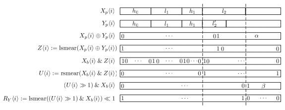
Figure 2: Computing $\mathrm{lnca}(X_{p}\langle{i}\rangle,Y_{p}\langle{i}\rangle)$. The solid lines in $X_{p}\langle{i}\rangle$ and $Y_{p}\langle{i}\rangle$ show part boundaries and the dashed lines show boundaries for $\mathrm{lcpp}(X_{p}\langle{i}\rangle,Y_{p}\langle{i}\rangle)$ and $\mathrm{ldp}_{Y_{p}\langle{i}\rangle}(X_{p}\langle{i}\rangle)$. $\alpha$ and $\beta$ are arbitrary bit strings.

The mask $Z\langle{i}\rangle$ consists of $1$’s in position $z=\mathrm{rmb}(X_{p}\langle{i}\rangle\oplus Y_{p}\langle{i}\rangle)$ and all positions to the left of $z$. Since $X_{p}$ and $Y_{p}$ are distinct labels, $z$ is the rightmost position where $X_{p}\langle{i}\rangle$ and $Y_{p}\langle{i}\rangle$ differ. Since the parts are prefix free encoded and prefixed with $0$, we have that $z$ is a position within $\mathrm{ldp}_{Y_{p}\langle{i}\rangle}(X_{p}\langle{i}\rangle)$ and $\mathrm{ldp}_{X_{p}\langle{i}\rangle}(Y_{p}\langle{i}\rangle)$ and it is not the leftmost position. Consequently, $u=\mathrm{lmb}(X_{b}\langle{i}\rangle\>\&\>Z\langle{i}\rangle)$ is the leftmost position of $\mathrm{ldp}_{Y_{p}\langle{i}\rangle}(X_{p}\langle{i}\rangle)$ and $\mathrm{ldp}_{X_{p}\langle{i}\rangle}(Y_{p}\langle{i}\rangle)$, and therefore the leftmost position to the right of $\mathrm{lcpp}(X_{p}\langle{i}\rangle,Y_{p}\langle{i}\rangle)$. Hence, $U\langle{i}\rangle=\mathrm{rsmear}(X_{b}\langle{i}\rangle\>\&\>Z\langle{i}\rangle)$ consists of $1$’s in all positions to the right of $\mathrm{lcpp}(X_{p}\langle{i}\rangle,Y_{p}\langle{i}\rangle)$. This implies that $\mathrm{lmb}(U\langle{i}\rangle\gg 1)\>\&\>X_{b}\langle{i}\rangle)$ is the position immediately to the right of $\mathrm{ldp}_{Y_{p}\langle{i}\rangle}(X_{p}\langle{i}\rangle)$ (if $\mathrm{ldp}_{Y_{p}\langle{i}\rangle}(X_{p}\langle{i}\rangle)$ is the rightmost part this still holds due to the extra bit in $X_{b}$ at the rightmost position). Therefore $R_{Y}\langle{i}\rangle:=\mathrm{lsmear}((U\langle{i}\rangle\gg 1)\>\&\>X_{b}\langle{i}\rangle)\ll 1$ consists of $1$’s in all positions of $\mathrm{lcpp}(X_{p}\langle{i}\rangle,Y_{p}\langle{i}\rangle)$ and $\mathrm{ldp}_{Y_{p}\langle{i}\rangle}(X_{p}\langle{i}\rangle)$. Symmetrically, $R_{X}\langle{i}\rangle:=\mathrm{lsmear}((U\langle{i}\rangle\gg 1)\>\&\>Y_{b}\langle{i}\rangle)\ll 1$ consists of $1$’s in all positions of $\mathrm{lcpp}(X_{p}\langle{i}\rangle,Y_{p}\langle{i}\rangle)$ and $\mathrm{ldp}_{X_{p}\langle{i}\rangle}(Y_{p}\langle{i}\rangle)$.

All operations except the elementwise $\mathrm{rsmear}$ in the computation of $U$ are straightforward to compute in $O(1)$ time. Hence, the time for this step is $O(\log f)$.

Step 2: Extract Relevants Parts

Compute the $f/3$-packed sequences $\mathrm{LCPP}$, $\mathrm{LDP}_{Y}$, $\mathrm{LDP}_{X}$, and $M$ given by

$$\mathrm{LCPP}\langle{i}\rangle :=X_{p}\langle{i}\rangle\>\&\>\overline{U\langle{i}\rangle}$$

$$\mathrm{LDP}_{Y}\langle{i}\rangle :=X_{p}\langle{i}\rangle\>\&\>R_{Y}\langle{i}\rangle\>\&\>U\langle{i}\rangle$$

$$\mathrm{LDP}_{X}\langle{i}\rangle :=Y_{p}\langle{i}\rangle\>\&\>R_{X}\langle{i}\rangle\>\&\>U\langle{i}\rangle$$

$$M\langle{i}\rangle :=\min(\mathrm{LDP}_{Y}\langle{i}\rangle,\mathrm{LDP}_{X}\langle{i}\rangle)$$

From the definition of the mask in step $1$, we have that $\mathrm{LCPP}\langle{i}\rangle=\mathrm{lcpp}(X_{p}\langle{i}\rangle,Y_{p}\langle{i}\rangle)$. The sequence $\mathrm{LDP}_{Y}\langle{i}\rangle$ is $X\langle{i}\rangle$ where all but $\mathrm{ldp}_{Y_{p}\langle{i}\rangle}(X_{p}\langle{i}\rangle)$ is zeroed and therefore $\mathrm{LDP}_{Y}\langle{i}\rangle=\mathrm{ldp}_{Y_{p}\langle{i}\rangle}(X_{p}\langle{i}\rangle)\gg|\mathrm{lcpp}(X_{p}\langle{i}\rangle,Y_{p}\langle{i}\rangle)|$ (see Figure 2). Similarly, $\mathrm{LDP}_{X}\langle{i}\rangle=\mathrm{ldp}_{X_{p}\langle{i}\rangle}(Y_{p}\langle{i}\rangle)\gg|\mathrm{lcpp}(X_{p}\langle{i}\rangle,Y_{p}\langle{i}\rangle)|$. The parts $\mathrm{ldp}_{Y_{p}\langle{i}\rangle}(X_{p}\langle{i}\rangle)$ and $\mathrm{ldp}_{X_{p}\langle{i}\rangle}(Y_{p}\langle{i}\rangle)$ are left aligned in $\mathrm{LDP}_{Y}\langle{i}\rangle$ and $\mathrm{LDP}_{X}\langle{i}\rangle$ and all other positions are $0$. Hence,

$$M\langle{i}\rangle=\min(\mathrm{LDP}_{Y}\langle{i}\rangle,\mathrm{LDP}_{X}\langle{i}\rangle)=\min_{\mathrm{lex}}(\mathrm{LDP}_{Y}\langle{i}\rangle,\mathrm{LDP}_{X}\langle{i}\rangle)\gg|\mathrm{lcpp}(X_{p}\langle{i}\rangle,Y_{p}\langle{i}\rangle)|.$$

The time for this step is $O(1)$.

Step 3: Construct Labels

The part labels are computed as the $f/3$-packed sequence $P$ given by

$$P\langle{i}\rangle=\begin{cases}\mathrm{LCPP}\langle{i}\rangle&\text{if $\mathrm{lsmear}(X_{b}\langle{i}\rangle\>\&\>U\langle{i}\rangle)=\mathrm{lsmear}(X_{l}\langle{i}\rangle\>\&\>U\langle{i}\rangle)$ },\\ \mathrm{LCPP}\langle{i}\rangle\mid M\langle{i}\rangle&\text{otherwise}.\end{cases}$$

Recall that $U\langle{i}\rangle$ consists of $1$’s at all position in of $1$’s in all positions to the right of $\mathrm{lcpp}(X_{p}\langle{i}\rangle,Y_{p}\langle{i}\rangle)$. Hence, if $\mathrm{lsmear}(X_{b}\langle{i}\rangle\>\&\>U\langle{i}\rangle)=\mathrm{lsmear}(X_{l}\langle{i}\rangle\>\&\>U\langle{i}\rangle)$, then $\mathrm{ldp}_{Y_{p}\langle{i}\rangle}(X_{p}\langle{i}\rangle)$ is a light part. By Lemma 11 it follows that $P\langle{i}\rangle$ is the part label for $\mathrm{lnca}(X\langle{i}\rangle,Y\langle{i}\rangle)$. To compute $P$, we compare the sequences $\mathrm{lsmear}(X_{b}\langle{i}\rangle\>\&\>U\langle{i}\rangle)$ and $\mathrm{lsmear}(X_{l}\langle{i}\rangle\>\&\>U\langle{i}\rangle)$, extract fields accordingly from $M$, and $\mid$ this with $\mathrm{LCPP}$. The remaining sublabels are constructed by extracting from $X_{b}$ and $X_{l}$ using $Z$. We construct the final $f$-packed sequence $\textsc{Lnca}(X,Y)$ by zipping the sublabels together.

The time for this step is $O(1)$.

The total time for the algorithm is $O(\log f)$. For general packed sequences, we have the following result.

Lemma 12

For $f$-packed sequences $X$ and $Y$ of length $r$, we can compute $\textsc{Lnca}(X,Y)$ in time $O(\frac{rf}{w}\log f+1)$.

Proof. Apply the algorithm from the proof of Lemma 2 using the $O(\log f)$ implementation of Lnca instruction. The time is $O(r\log f/s+1)=O(\frac{rf}{w}\log f+1)$. $\Box$

6.5 The Algorithm

We combine the implementation of Map and Lnca with Lemma 1 to obtain the following result.

Theorem 4

Approximate string matching for strings $P$ and $Q$ of lengths $m$ and $n$, respectively, with error threshold $k$ can be solved in time $O(nk\cdot\frac{\log^{2}m\log w}{w}+n)$ and space $O(m)$.

Proof. We plug in the results for Map and Lnca from Lemmas 12 and 10 into the reduction from Lemma 1. We have $r,u=O(m)$ and $f=O(\log m)$ and therefore $s=p=O(m)$ and $q=O(\frac{rf}{w}\log r\log w+\frac{(r+u)f}{w}\log w+\frac{rf}{w}\log f+1)=O(\frac{m\log^{2}m\log w}{w}+1)$. Thus, we obtain an algorithm for approximate string matching using space $O(m)$ and time $O(\frac{nk}{m}\cdot\frac{m\log^{2}m\log w}{w}+n)=O(nk\cdot\frac{\log^{2}m\log w}{w}+n)$. $\Box$
Combining Theorems 3 and 4 we have shown Theorem 1.

7 Acknowledgments

We would like to thank the anonymous reviewers for many valuable comments that greatly improved the quality of the paper.

References

- [1] S. Albers and T. Hagerup. Improved parallel integer sorting without concurrent writing. Inform. and Comput., 136:25–51, 1997.
- [2] S. Alstrup, C. Gavoille, H. Kaplan, and T. Rauhe. Nearest common ancestors: A survey and a new algorithm for a distributed environment. Theory Comput. Syst., 37:441–456, 2004.
- [3] A. Andersson, T. Hagerup, S. Nilsson, and R. Raman. Sorting in linear time? J. Comput. System Sci., 57(1):74–93, 1998.
- [4] V. L. Arlazarov, E. A. Dinic, M. A. Kronrod, and I. A. Faradzev. On economic construction of the transitive closure of a directed graph (in russian). english translation in soviet math. dokl. 11, 1209-1210, 1975. Dokl. Acad. Nauk., 194:487–488, 1970.
- [5] R. Baeza-Yates and G. H. Gonnet. A new approach to text searching. Commun. ACM, 35(10):74–82, 1992.
- [6] R. A. Baeza-Yates and G. Navarro. A faster algorithm for approximate string matching. In Proceedings of the 7th Annual Symposium on Combinatorial Pattern Matching, Lecture Notes in Computer Science, volume 1075, pages 1–23, 1996.
- [7] K. E. Batcher. Sorting networks and their applications. In Proceedings of the AFIPS Spring Joint Computer Conference, pages 307–314, 1968.
- [8] M. A. Bender and M. Farach-Colton. The LCA problem revisited. In Proceedings of the 4th Latin American Symposium on Theoretical Informatics, pages 88–94, 2000.
- [9] P. Bille and M. Farach-Colton. Fast and compact regular expression matching. Theoret. Comput. Sci., 409:486 – 496, 2008.
- [10] R. Cole and R. Hariharan. Approximate string matching: A simpler faster algorithm. SIAM J. Comput., 31(6):1761–1782, 2002.
- [11] T. H. Cormen, C. E. Leiserson, R. L. Rivest, and C. Stein. Introduction to Algorithms, second edition. MIT Press, 2001.
- [12] M. Farach-Colton, P. Ferragina, and S. Muthukrishnan. On the sorting-complexity of suffix tree construction. J. ACM, 47(6):987–1011, 2000.
- [13] Z. Galil and R. Giancarlo. Data structures and algorithms for approximate string matching. J. Complexity, 4(1):33–72, 1988.
- [14] Z. Galil and K. Park. An improved algorithm for approximate string matching. SIAM J. Comput., 19(6):989–999, 1990.
- [15] D. Gusfield. Algorithms on strings, trees, and sequences: computer science and computational biology. Cambridge, 1997.
- [16] T. Hagerup. Sorting and searching on the word RAM. In Proceedings of the 15th Annual Symposium on Theoretical Aspects of Computer Science, Lecture Notes in Computer Science, volume 1373, pages 366–398, 1998.
- [17] D. Harel and R. E. Tarjan. Fast algorithms for finding nearest common ancestors. SIAM J. Comput., 13(2):338–355, 1984.
- [18] H. Hyyrö and G. Navarro. Bit-parallel witnesses and their applications to approximate string matching. Algorithmica, 41(3):203–231, 2005.
- [19] D. E. Knuth. The Art of Computer Programming, Volume 4, Pre-Fascicle 1a: Bitwise Tricks and Techniques (Art of Computer Programming). 2008.
- [20] G. M. Landau and U. Vishkin. Fast parallel and serial approximate string matching. J. Algorithms, 10:157–169, 1989.
- [21] F. T. Leighton. Introduction to Parallel Algorithms and Architectures: Arrays, Trees, Hypercubes. Morgan Kaufmann Publishers, 1992.
- [22] W. Masek and M. Paterson. A faster algorithm for computing string edit distances. J. Comput. System Sci., 20:18–31, 1980.
- [23] E. W. Myers. An difference algorithm and its variations. Algorithmica, 1(2):251–266, 1986.
- [24] G. Myers. A fast bit-vector algorithm for approximate string matching based on dynamic programming. J. ACM, 46(3):395–415, 1999.
- [25] G. Navarro. A guided tour to approximate string matching. ACM Comput. Surv., 33(1):31–88, 2001.
- [26] S. C. Sahinalp and U. Vishkin. Efficient approximate and dynamic matching of patterns using a labeling paradigm. In Proceedings of the 37th Annual Symposium on Foundations of Computer Science, pages 320–328, Washington, DC, USA, 1996. IEEE Computer Society.
- [27] P. Sellers. The theory and computation of evolutionary distances: Pattern recognition. J. Algorithms, 1:359–373, 1980.
- [28] E. Ukkonen. Algorithms for approximate string matching. Inf. Control, 64(1-3):100–118, 1985.
- [29] E. Ukkonen and D. Wood. Approximate string matching with suffix automata. Algorithmica, 10(5):353–364, 1993.
- [30] R. A. Wagner and M. J. Fischer. The string-to-string correction problem. J. ACM, 21:168–173, 1974.
- [31] A. H. Wright. Approximate string matching using within-word parallelism. Softw. Pract. Exper., 24(4):337–362, 1994.
- [32] S. Wu and U. Manber. Fast text searching: allowing errors. Commun. ACM, 35(10):83–91, 1992.