Localized magnetic states in biased bilayer and trilayer graphene

Abstract

We study the localized magnetic states of impurity in biased bilayer and trilayer graphene. It is found that the magnetic boundary for bilayer and trilayer graphene presents the mixing features of Dirac and conventional fermion. For zero gate bias, as the impurity energy approaches the Dirac point, the impurity magnetization region diminishes for bilayer and trilayer graphene. When a gate bias is applied, the dependence of impurity magnetic states on the impurity energy exhibits a different behavior for bilayer and trilayer graphene due to the opening of a gap between the valence and the conduction band in the bilayer graphene with the gate bias applied. The magnetic moment and the corresponding magnetic transition of the impurity in bilayer graphene are also investigated.

I Introduction

The intense research currently devoted to graphene, a two-dimensional carbon honeycomb lattice, has uncovered a wealth of fascinating properties such as the anomalous quantized Hall effect, the absence of the weak localization and existence of the minimal conductivitynovoselov2 ; zhang ; geim ; castrocond ; novoselovsci2004 . Graphene has a high mobility, its carrier density is controllable by an applied gate voltagezhang and a spin-orbit interactionberger ; huertas ; kane1 ; yao ; ding1 .

Graphene structures have been the focus of much interest Ponomarenko ; Pedersenprl2008 ; Novoselovnat2006 ; Castroprl2008 ; Castroprl20082 ; Bostwicknjp ; han2007 ; Wimmerprl2008 ; Wangarxiv ; guonano2007 . In particular, adatoms may be positioned on graphene by current nanotechnologyeiglernature1990 , rendering the study and manipulation of local electronic properties. Ab initio calculations for transition metal adatomsduffyprb1998 show a tendency to the formation of local magnetic moments. Recently Uchoa et al.Uchoaprl2008 examined the condition for the emergence of localized magnetic moment on adatoms with inner shell electrons on a single layer graphene. It is found that the impurity magnetization boundary exhibits anomalous characteristics. In contrast to the case of an impurity in an ordinary metal, the impurity can magnetize for any small charging energy due to the low density of state(DOS) at the Dirac point. On the other hand, detailed experimental studies Bostwicknjp on multi-layer graphene showed a marked modification of the electronic structure with the number of layers. Hence, we expect ding2 a qualitative difference in the magnetic properties of the adatoms on multilayer graphene; an issue which we address here by inspecting the localized magnetic state of an impurity in a biased bilayer and trilayer graphene. We find that the size of the magnetic region decreases rapidly compared with that in monolayer graphene, the impurity can magnetize even when the energy of the doubly occupied state is below the Fermi level, and the impurity magnetization region is asymmetric due to the special nature of the quasiparticles having mixed features of Dirac and conventional fermions. When a gate bias is applied, the dependence of the impurity magnetic states on the impurity energy for a bilayer graphene exhibits a different behavior from that for a trilayer graphene due to the opening of a gate-induced gap between the valence and the conduction band in the bilayer graphene. Calculating the occupation of the impurity level and the susceptibility in the bilayer graphene we show that the magnetic moment decreases with increasing the inter-layer coupling.

II Bilayer graphene

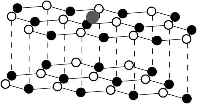
Figure 1: Schematic diagram of the lattice structure of the bilayer graphene with an impurity atom.

Fig.1 shows the lattice structure of the bilayer graphene with the adatom. The inter-layer stacking is assumed to be the Bernal order where the top layer has its A sublattice atop the sublattice B of the bottom layer. The bias voltage $V$ is applied across the layers. The system Hamiltonian

$$H=H_{TB}+H_{i}+H_{f}$$ (1)

contains the graphene bilayer term $H_{TB}$, which in a tight-binding approximation reads

$$H_{TB}=\sum\limits_{l=1}^{2}H_{l}+H_{T}+H_{V},$$ (2)

with

$$H_{l}=-t\sum\limits_{\langle i,j\rangle\sigma}[a_{l\sigma}^{\dagger}(\mathbf{R}_{i})b_{l\sigma}(\mathbf{R}_{j})+b_{l\sigma}^{\dagger}(\mathbf{R}_{j})a_{l\sigma}(\mathbf{R}_{i})],$$ (3)

$$H_{T}=-t_{p}\sum\limits_{i,\sigma}[a_{1\sigma}^{\dagger}(\mathbf{R}_{i})b_{2\sigma}(\mathbf{R}_{i})+b_{2\sigma}^{\dagger}(\mathbf{R}_{i})a_{1\sigma}(\mathbf{R}_{i})],$$ (4)

$$H_{V}=\frac{V}{2}\sum_{i\sigma}[a_{1\sigma}^{\dagger}(\mathbf{R}_{i})a_{1\sigma}(\mathbf{R}_{i})+b_{1\sigma}^{\dagger}(\mathbf{R}_{i})b_{1\sigma}(\mathbf{R}_{i})-a_{2\sigma}^{\dagger}(\mathbf{R}_{i})a_{2\sigma}(\mathbf{R}_{i})-b_{2\sigma}^{\dagger}(\mathbf{R}_{i}).b_{2\sigma}(\mathbf{R}_{i})],$$ (5)

The operator $a_{l\sigma}(\mathbf{R}_{i})\;(b_{l\sigma}(\mathbf{R}_{i}))$ annihilates a state with a spin $\sigma$ at the position $\mathbf{R}_{i}$ on the sublattice A(B) of the $l$ plane. $t$ is the nearest neighbour in-plane hopping energy, $t_{p}$ is the inter-layer hopping energy. For the hybridization with the localized impurity states we write

$$H_{i}=V_{f}\sum\limits_{\sigma}[f_{\sigma}^{\dagger}b_{1\sigma}(0)+b_{1\sigma}^{\dagger}(0)f_{\sigma}],$$ (6)

where $f_{\sigma}(f_{\sigma}^{\dagger})$ is the annihilation (creation) operator of a state with a spin $\sigma$ at the impurity, and $V_{f}$ is the hybridization strength. In the momentum space we have

$$H_{l}=-t\sum\limits_{\mathbf{k}\sigma}[\phi(\mathbf{k})a_{l\mathbf{k}\sigma}^{\dagger}b_{l\mathbf{k}\sigma}+\phi^{*}(\mathbf{k})b_{l\mathbf{k}\sigma}^{\dagger}a_{l\mathbf{k}\sigma}],$$ (7)

$$H_{T}=t_{p}\sum\limits_{\mathbf{k},\sigma}[a_{1\mathbf{k}\sigma}^{\dagger}b_{2\mathbf{k}\sigma}+b_{2\mathbf{k}\sigma}^{\dagger}a_{1\mathbf{k}\sigma}],$$ (8)

$$H_{V}=\frac{V}{2}\sum_{\mathbf{k}\sigma}[a_{1\mathbf{k}\sigma}^{\dagger}a_{1\mathbf{k}\sigma}+b_{1\mathbf{k}\sigma}^{\dagger}b_{1\mathbf{k}\sigma}-a_{2\mathbf{k}\sigma}^{\dagger}a_{2\mathbf{k}\sigma}-b_{2\mathbf{k}\sigma}^{\dagger}b_{2\mathbf{k}\sigma}],$$ (9)

$$H_{i}=\frac{V_{f}}{\sqrt{N}}\sum\limits_{\mathbf{k}\sigma}(f_{\sigma}^{\dagger}b_{1\mathbf{k}\sigma}+b_{1\mathbf{k}\sigma}^{\dagger}f_{\sigma}),$$ (10)

where $\phi(\mathbf{q})=-t\sum\limits_{i=1}^{3}e^{i\mathbf{q}\cdot\mathbf{\delta_{i}}}$ with $\delta_{1}=\frac{a}{2}(1,\sqrt{3},0),\delta_{2}=\frac{a}{2}(1,-\sqrt{3},0),\delta_{3}=a(1,0,0)$ (here $a$ is the lattice spacing), and $N$ is the number of sites on sublattice B of plane 1. Diagonalizing $H_{TB}$ we find the spectrum

$$E_{\pm\pm}(\mathbf{k})=\pm\sqrt{\epsilon_{k}^{2}+\frac{t_{p}^{2}}{2}+\frac{V^{2}}{4}\pm\sqrt{\frac{t_{p}^{4}}{4}+(t_{p}^{2}+V^{2})\epsilon_{k}^{2}}},$$ (11)

where $\epsilon_{k}=\pm|\phi(\mathbf{k})|$ is linearizable around the $\mathbf{K}$ points of the Brillouin zone by $\epsilon_{k}=\pm v_{F}|\mathbf{k}|$ where $v_{F}=3ta/2$ is the Fermi velocity. The impurity is described by Hamiltonian $H_{f}$ with

$$H_{f}=\sum\limits_{\sigma}\varepsilon_{0}f^{\dagger}_{\sigma}f_{\sigma}+Un_{\uparrow}n_{\downarrow},$$ (12)

where $n_{\sigma}=f_{\sigma}^{\dagger}f_{\sigma}$ is the occupation number operator, $\varepsilon_{0}$ is the single electron energy at the impurity. The Coulomb interaction is included as a finite Anderson term $U$. For simplicity, we adopt a mean field approximation to the electronic correlations at the impurity, $Un_{\uparrow}n_{\downarrow}\simeq U\sum\limits_{\sigma}\langle n_{\overline{\sigma}}\rangle f_{\sigma}^{\dagger}f_{\sigma}-U\langle n_{\uparrow}\rangle\langle n_{\downarrow}\rangle$. The impurity Hamiltonian is rewritten as $H_{f}=\sum\limits_{\sigma}\varepsilon_{\sigma}f^{\dagger}_{\sigma}f_{\sigma}$ with $\varepsilon_{\sigma}=\varepsilon_{0}+U\langle n_{\overline{\sigma}}\rangle$. To investigate the localized magnetic states, we calculate the occupation number of the electrons of a given spin $\sigma$ at the impurity. At low temperatures all the states below the Fermi level $\mu$ are completely occupied and the occupation of the impurity is determined by

$$\langle n_{\sigma}\rangle=\int_{-\infty}^{\mu}d\omega\rho_{f}^{\sigma}(\omega),$$ (13)

where $\rho_{f}^{\sigma}(\omega)$ is DOS at the impurity level. We infer it from the retarded Green’s function

$$G_{f}^{r,\sigma\sigma^{\prime}}(t-t^{\prime})=-i\theta(t-t^{\prime})\langle\{f_{\sigma}(t),f_{\sigma^{\prime}}^{\dagger}(t^{\prime})\}\rangle.$$ (14)

By the standard equation of motion, we can derive

$$G_{f}^{r,\sigma\sigma^{\prime}}(\omega)=\frac{\delta_{\sigma\sigma^{\prime}}}{\omega-\varepsilon_{\sigma}-\Sigma_{f}^{r}(\omega)+i\eta},$$ (15)

where

$$\begin{array}[]{cll}\Sigma_{f}^{r}(\omega)&=&\frac{V_{f}^{2}}{N}\sum\limits_{\mathbf{k}}\frac{-(\omega-\frac{V}{2})v_{F}^{2}|\mathbf{k}|^{2}+(\omega-\frac{V}{2})(\omega+\frac{V}{2})^{2}-t_{p}^{2}(\omega+\frac{V}{2})}{v_{F}^{4}|\mathbf{k}|^{4}-2(\omega^{2}+\frac{V^{2}}{4})v_{F}^{2}|\mathbf{k}|^{2}+(\omega^{2}-\frac{V^{2}}{2})^{2}-t_{p}^{2}(\omega^{2}-\frac{V^{2}}{4})}.\end{array}$$ (16)

Introducing a high-energy cutoff $D$ of the graphene bandwidth, we obtain for $\omega^{2}\geq\frac{1}{4}\frac{t_{p}^{2}V^{2}}{t_{p}^{2}+V^{2}}$,

$$\begin{array}[]{cll}\Sigma_{f}^{r}(\omega)&=&\frac{V_{f}^{2}}{D^{2}}\{\frac{V\omega^{2}-(V^{2}/2+t_{p}^{2})\omega-Vt_{p}^{2}/2}{\sqrt{4(V^{2}+t_{p}^{2})\omega^{2}-t_{p}^{2}V^{2}}}\ln|\frac{(D^{2}-x_{1})x_{2}}{(D^{2}-x_{2})x_{1}}|-\frac{\omega-V/2}{2}\ln|\frac{(D^{2}-x_{1})(D^{2}-x_{2})}{x_{1}x_{2}}|\}\\ &&+i\frac{\pi V_{f}^{2}}{D^{2}}\{\frac{V\omega^{2}-(V^{2}/2+t_{p}^{2})\omega-Vt_{p}^{2}/2}{\sqrt{4(V^{2}+t_{p}^{2})\omega^{2}-t_{p}^{2}V^{2}}}[\text{sgn}(\frac{dx_{1}}{d\omega})\theta(0<x_{1}<D^{2})-\text{sgn}(\frac{dx_{2}}{d\omega})\theta(0<x_{2}<D^{2})]\\ &&-\frac{\omega-V/2}{2}[\text{sgn}(\frac{dx_{1}}{d\omega})\theta(0<x_{1}<D^{2})+\text{sgn}(\frac{dx_{2}}{d\omega})\theta(0<x_{2}<D^{2})]\},\end{array}$$ (17)

where $\theta(x)$ is the step function, and

$$x_{1,2}=(\omega^{2}+\frac{V^{2}}{4})\pm\frac{1}{2}\sqrt{4(V^{2}+t_{p}^{2})\omega^{2}-t_{p}^{2}V^{2}}.$$ (18)

For $\omega^{2}<\frac{1}{4}\frac{t_{p}^{2}V^{2}}{t_{p}^{2}+V^{2}}$,

$$\begin{array}[]{cll}\Sigma_{f}^{r}(\omega)&=&\frac{V_{f}^{2}}{D^{2}}[-\frac{\omega-V/2}{2}\ln|\frac{D^{4}-2(\omega^{2}+V^{2}/4)D^{2}+(\omega^{2}-V^{2}/2)^{2}-t_{p}^{2}(\omega^{2}-V^{2}/4)}{(\omega^{2}-V^{2}/2)^{2}-t_{p}^{2}(\omega^{2}-V^{2}/4)}|\\ &&+\frac{V\omega^{2}-(V^{2}/2+t_{p}^{2})\omega-Vt_{p}^{2}/2}{\sqrt{t_{p}^{2}V^{2}/4-(V^{2}+t_{p}^{2})\omega^{2}}}(\arctan\frac{D^{2}-\omega^{2}-V^{2}/4}{\sqrt{t_{p}^{2}V^{2}/4-(V^{2}+t_{p}^{2})\omega^{2}}}+\arctan\frac{\omega^{2}+V^{2}/4}{\sqrt{t_{p}^{2}V^{2}/4-(V^{2}+t_{p}^{2})\omega^{2}}})].\\ \end{array}$$ (19)

The summation over $\mathbf{k}$ in Eq.(16) is accurate for $\omega\ll D$ by ensuring the conservation of the total number of states in the Brillouin zone according to the Debye’s prescription. Substituting $\Sigma_{f}^{r}(\omega)$ into Eq.(15), the retarded Green’s function $G_{f}^{r,\sigma\sigma}(\omega)$ can be obtained. Note, the determination of $\langle n_{\sigma}\rangle$ in Eq.(13) entails a self-consistent calculation of DOS at the impurity level via the relation $\rho_{f}^{\sigma}(\omega)=-\frac{1}{\pi}\text{Im}G_{f}^{r,\sigma\sigma}(\omega)$. When $t_{p}=V=0$, our present results reduce to those of Ref.Uchoaprl2008 .

III Trilayer graphene

The Hamiltonian for trilayer graphene contains a coupling the B atom of the second layer to the A atom of the third layer according to the conventional Bernal-type stacking order. Similar to the bilayer graphene case we find for the impurity Green’s function

$$G_{f}^{r,\sigma\sigma^{\prime}}(\omega)=\frac{\delta_{\sigma\sigma^{\prime}}}{\omega-\epsilon_{\sigma}-\Sigma^{r}+i\eta},$$ (20)

where

$$\begin{array}[]{cll}\Sigma^{r}&=&-\frac{V_{f}^{2}}{N}\sum\limits_{\mathbf{k}}\frac{A_{1}v_{F}^{4}|\mathbf{k}|^{4}+B_{1}v_{F}^{2}|\mathbf{k}|^{2}+C_{1}}{v_{F}^{6}|\mathbf{k}|^{6}+B_{2}v_{F}^{4}|\mathbf{k}|^{4}+C_{2}v_{F}^{2}|\mathbf{k}|^{2}+D_{2}}\end{array}$$ (21)

with $A_{1}=\omega-\frac{V}{2}$, $B_{1}=t_{p}^{2}\omega-(\omega-\frac{V}{2})[\omega^{2}+(\omega+\frac{V}{2})^{2}]$, $C_{1}=\omega^{2}(\omega-\frac{V}{2})(\omega+\frac{V}{2})^{2}-2t_{p}^{2}\omega^{2}(\omega+\frac{V}{2})$, $B_{2}=-3\omega^{2}-\frac{V^{2}}{2}$, $C_{2}=-2t_{p}^{2}\omega^{2}+3\omega^{4}+\frac{V^{4}}{16}$, $D_{2}=-\omega^{2}(\omega^{2}-\frac{V^{2}}{4})^{2}+2t_{p}^{2}\omega^{2}(\omega^{2}-\frac{V^{2}}{4})$. Performing the summation over $\mathbf{k}$ in Eq.(21) as Eq.(16) we find for $\Delta=(2B_{2}^{3}-9B_{2}C_{2}+27D_{2})^{2}+4(-B_{2}^{2}+3C_{2})^{3}\geq 0$ the result

$$\begin{array}[]{cll}\Sigma^{r}&=&-\frac{V_{f}^{2}}{D^{2}}\{[A_{1}+\frac{A_{1}(x_{2}+x_{3})x_{1}+B_{1}x_{1}-A_{1}x_{2}x_{3}+C_{1}}{(x_{2}-x_{1})(x_{3}-x_{1})}]\ln|\frac{D^{2}-x_{1}}{x_{1}}|\\ &&+\frac{A_{1}(x_{2}+x_{3})+B_{1}}{\sqrt{x_{2}x_{3}-(x_{2}+x_{3})^{2}/4}}(\arctan\frac{D^{2}-(x_{2}+x_{3})/2}{\sqrt{x_{2}x_{3}-(x_{2}+x_{3})^{2}/4}}+\arctan\frac{(x_{2}+x_{3})/2}{\sqrt{x_{2}x_{3}-(x_{2}+x_{3})^{2}/4}})\\ &&+\frac{A_{1}(x_{2}+x_{3})x_{1}+B_{1}x_{1}-A_{1}x_{2}x_{3}+C_{1}}{(x_{2}-x_{1})(x_{3}-x_{1})}[\frac{-1}{2}\ln\frac{D^{2}-(x_{2}+x_{3})+x_{2}x_{3}}{x_{2}x_{3}}\\ &&+\frac{(x_{2}+x_{3})/2-x_{1}}{2\sqrt{x_{2}x_{3}-(x_{2}+x_{3})^{2}/4}}(\arctan\frac{D^{2}-(x_{2}+x_{3})/2}{\sqrt{x_{2}x_{3}-(x_{2}+x_{3})^{2}/4}}+\arctan\frac{(x_{2}+x_{3})/2}{\sqrt{x_{2}x_{3}-(x_{2}+x_{3})^{2}/4}})]\}\\ &&-i\text{sgn}(\frac{dx_{1}}{d\omega})\theta(0<x_{1}<D^{2})\frac{\pi V_{f}^{2}}{D^{2}}[A_{1}+\frac{A_{1}(x_{2}+x_{3})x_{1}+B_{1}x_{1}-A_{1}x_{2}x_{3}+C_{1}}{(x_{2}-x_{1})(x_{3}-x_{1})}],\end{array}$$ (22)

where

$$\begin{array}[]{cll}x_{1}&=&-\frac{B_{2}}{3}+\frac{1}{2^{1/3}}\frac{1}{3}\{-2B_{2}^{3}+9B_{2}C_{2}-27D_{2}+\sqrt{(2B_{2}^{3}-9B_{2}C_{2}+27D_{2})^{2}+4(-B_{2}^{2}+3C_{2})^{3}}\}^{\frac{1}{3}}\\ &&+\frac{1}{2^{1/3}3}\{-2B_{2}^{3}+9B_{2}C_{2}-27D_{2}-\sqrt{(2B_{2}^{3}-9B_{2}C_{2}+27D_{2})^{2}+4(-B_{2}^{2}+3C_{2})^{3}}\}^{\frac{1}{3}},\end{array}$$ (23)

$$\begin{array}[]{cll}x_{2,3}&=&-\frac{B_{2}}{3}+\frac{-\frac{1}{2}-i\frac{\sqrt{3}}{2}}{3}\frac{1}{2^{1/3}}\{-2B_{2}^{3}+9B_{2}C_{2}-27D_{2}\pm\sqrt{(2B_{2}^{3}-9B_{2}C_{2}+27D_{2})^{2}+4(-B_{2}^{2}+3C_{2})^{3}}\}^{\frac{1}{3}}\\ &&+\frac{-\frac{1}{2}+i\frac{\sqrt{3}}{2}}{3}\frac{1}{2^{1/3}}\{-2B_{2}^{3}+9B_{2}C_{2}-27D_{2}\mp\sqrt{(2B_{2}^{3}-9B_{2}C_{2}+27D_{2})^{2}+4(-B_{2}^{2}+3C_{2})^{3}}\}^{\frac{1}{3}}.\end{array}$$ (24)

For $\Delta<0$,

$$\begin{array}[]{cll}&&\Sigma^{r}\\ &=&-\frac{V_{f}^{2}}{D^{2}}\{[A_{1}+\frac{[A_{1}(x_{2}+x_{3})+B_{1}]x_{1}-A_{1}x_{2}x_{3}+C_{1}}{(x_{2}-x_{1})(x_{3}-x_{1})}]\ln|\frac{D^{2}-x_{1}}{x_{1}}|\\ &&-[\frac{A_{1}(x_{2}+x_{3})+B_{1}}{x_{3}-x_{2}}+\frac{[A_{1}(x_{2}+x_{3})+B_{1}]x_{1}-A_{1}x_{2}x_{3}+C_{1}}{(x_{2}-x_{1})(x_{3}-x_{2})}]\ln|\frac{D^{2}-x_{2}}{x_{2}}|\\ &&+[\frac{A_{1}(x_{2}+x_{3})+B_{1}}{x_{3}-x_{2}}+\frac{[A_{1}(x_{2}+x_{3})+B_{1}]x_{1}-A_{1}x_{2}x_{3}+C_{1}}{(x_{2}-x_{1})(x_{3}-x_{2})}-\frac{[A_{1}(x_{2}+x_{3})+B_{1}]x_{1}-A_{1}x_{2}x_{3}+C_{1}}{(x_{2}-x_{1})(x_{3}-x_{1})}]\ln|\frac{D^{2}-x_{3}}{x_{3}}|\}\\ &&-i\frac{\pi V_{f}^{2}}{D^{2}}\{\text{sgn}(\frac{dx_{1}}{d\omega})\theta(0<x_{1}<D^{2})[A_{1}+\frac{[A_{1}(x_{2}+x_{3})+B_{1}]x_{1}-A_{1}x_{2}x_{3}+C_{1}}{(x_{2}-x_{1})(x_{3}-x_{1})}]\\ &&-\text{sgn}(\frac{dx_{2}}{d\omega})\theta(0<x_{2}<D^{2})[\frac{A_{1}(x_{2}+x_{3})+B_{1}}{x_{3}-x_{2}}+\frac{[A_{1}(x_{2}+x_{3})+B_{1}]x_{1}-A_{1}x_{2}x_{3}+C_{1}}{(x_{2}-x_{1})(x_{3}-x_{2})}]\\ &&+\text{sgn}(\frac{dx_{3}}{d\omega})\theta(0<x_{3}<D^{2})[\frac{A_{1}(x_{2}+x_{3})+B_{1}}{x_{3}-x_{2}}+\frac{[A_{1}(x_{2}+x_{3})+B_{1}]x_{1}-A_{1}x_{2}x_{3}+C_{1}}{(x_{2}-x_{1})(x_{3}-x_{2})}-\frac{[A_{1}(x_{2}+x_{3})+B_{1}]x_{1}-A_{1}x_{2}x_{3}+C_{1}}{(x_{2}-x_{1})(x_{3}-x_{1})}]\},\end{array}$$ (25)

where

$$\begin{array}[]{cll}x_{1}&=&-\frac{B_{2}}{3}+\frac{2\sqrt{B_{2}^{2}-3C_{2}}}{3}\cos(\frac{\arccos T}{3}),\ \ \ x_{2}=-\frac{B_{2}}{3}+\frac{2\sqrt{B_{2}^{2}-3C_{2}}}{3}\cos(\frac{2\pi+\arccos T}{3}),\end{array}$$ (26)

$$\begin{array}[]{cll}x_{3}=-\frac{B_{2}}{3}+\frac{2\sqrt{B_{2}^{2}-3C_{2}}}{3}\cos(\frac{4\pi+\arccos T}{3}),\ \ \ T=-\frac{2(B_{2}^{2}-3C_{2})B_{2}-3(B_{2}C_{2}-9D_{2})}{2(B_{2}^{2}-3C_{2})^{\frac{3}{2}}}.\end{array}$$ (27)

Substituting Eqs.(22) and (25) in Eq.(20), we can derive self-consistently the occupation on the impurity for case of a trilayer graphene.

IV Numerical analysis

From the occupation of the two spin channel on the impurity we conclude on the formation of localized magnetic moment whenever $n_{\uparrow}\neq n_{\downarrow}$. For a detailed study conventionally, one introduces the dimensionless parameters

$$x=D\Gamma/U\;\mbox{ and }\;y=(\mu-\varepsilon_{0})/U\;\mbox{ with }\;\Gamma=\pi V_{f}^{2}/D^{2}.$$ (28)

The transition curves from the magnetic to the non-magnetic behavior as a function of the parameters $x$ and $y$ for the different hybridization and inter-layer coupling in the bilayer graphene are shown in Fig.2. For $t_{p}=V=0$, our results reduce to those of Ref.Uchoaprl2008 : The magnetic boundary exhibits an asymmetry around $y=0.5$, and can even cross when line $y=1$. The magnetic region shrinks in the $x$ direction with the hybridization $V_{f}$ is increased; for $y$ close to $1$ (cf. eq.(28)), the boundary line for magnetic transition shifts away from the $y$ axis due to the increased influence of graphene on the impurity magnetization with enhanced hybridization. When the inter-layer coupling $t_{p}$ is taken into account (see Fig.2(b)), the size of the magnetic region diminishes rapidly, and for a large enough $t_{p}$, the magnetic boundary shrinks above the line $y=0$. However, the magnetic boundary does not turn symmetric around $y=0.5$, and the above magnetic boundary line crosses the line $y=1$. The origin of this phenomena lies in the peculiar nature of the quasiparticles in the bilayer graphene; they exhibits features akin both to Dirac and to conventional fermions. The contribution of conventional fermions originates from the interlayer coupling that supports a metallic bilayer graphene and results in effects as for a conventional metallic host on the magnetic properties of the impurity. For large interlayer coupling we observe therefore magnetic boundaries similar an impurity in an ordinary metal. (Fig.3) shows for a bilayer graphene the boundary between magnetic and non-magnetic impurity states as a function of the parameters $x$ and $y$ (eq.28) for different impurity energy levels $\varepsilon_{0}$. For $V=0$ the size of the magnetic region grows as $\varepsilon_{0}$ approaches the energy of the Dirac point. This behavior is reminiscent of the single layer of grapheneUchoaprl2008 , and originates from the suppression of the DOS around the impurity energy level. In contrast, for a nonzero gate bias, when $\varepsilon_{0}$ is close to the Dirac point from the positive energy side, the size of the region first increases to the maximum, then decreases with decreasing $\varepsilon_{0}$, as shown in Fig.3(b). The explanation for this phenomenon is as follows: the gate bias voltage gives rise to a finite electronic gap between the conduction and the valence band, and induces a large local DOS close to the gap edgesEduardo . In particular, the DOS may extend into the gap due to the influence of the impurityNilssonprl . In this situation, the coupling between the bath and the impurity is enhanced inside the gap as compared with the zero bias case, leading thus to the non-monotonic dependence of the size of the region with $\varepsilon_{0}$.

Fig.4 shows the magnetic transition curve as a function of the parameters $x$ and $y$ (eq.28) for different $\varepsilon_{0}$ in the trilayer graphene. For $V=0$, phenomena such as the asymmetry around the line $y=0.5$ and the crossing of the line $y=1$ in the magnetic boundary suggest the existence of Dirac fermions in the trilayer graphene. As $\varepsilon_{0}$ approaches the energy of the Dirac point, the magnetization region of the impurity grows due to the two almost-linear touched bands reminiscent of the bands in monolayer grapheneBostwicknjp . It is interesting to note that for nonzero gate bias, the impurity magnetization region increases monotonously when $\varepsilon_{0}$ is close to the Dirac point, which is clearly different from that in the bilayer graphene. This behavior stems from the fact that the gate bias can not destroy the particle-hole degeneracy in the trilayer grapheneBostwicknjp .

To investigate the localized magnetic moment of the impurity in the magnetic region and the magnetic transition we calculate the magnetic susceptibility. The energy of the impurity spin states in a magnetic field $B$ is $\varepsilon_{\sigma}=\varepsilon_{0}-\sigma\mu_{B}B+Un_{\overline{\sigma}}$. The magnetic susceptibility of the impurity derives from

$$\chi=-\mu_{B}^{2}\sum\limits_{\sigma}\frac{d\langle n_{\sigma}\rangle}{d\varepsilon_{\sigma}}\frac{1-U\frac{d\langle n_{\overline{\sigma}}\rangle}{d\varepsilon_{\overline{\sigma}}}}{1-U^{2}\frac{d\langle n_{\overline{\sigma}}\rangle}{d\varepsilon_{\overline{\sigma}}}\frac{d\langle n_{\sigma}\rangle}{d\varepsilon_{\sigma}}}.$$ (29)

Fig.5 shows the occupation of the impurity spin level and the magnetic susceptibility as a function of $y$ for the different inter-layer coupling in a bilayer graphene. The occupation $\langle n_{\sigma}\rangle$ versus $y$ is a bubble that corresponds to the impurity magnetization. The corresponding susceptibility exhibits two peaks at the magnetization edge indicating the strength of the magnetic transition. For $t_{p}=0$, a strong magnetic moment of $\sim 0.7\mu_{B}$ forms in almost the whole magnetic region. With increasing the inter-layer coupling $t_{p}$, the magnetic bubble region diminishes signalling the decrease of the magnetic moment of the impurity, and the magnetic transition becomes very sharp. There is no localized magnetic moment in the case of a sufficiently strong inter-layer coupling. In this case, the magnetic boundary shrinks below the line $x=6$ in the $x$ direction(see Fig.2(b)). Fig.6 shows the occupation of the impurity level and the magnetic susceptibility as a function of $y$ for the different impurity energy level $\varepsilon_{0}$ in the bilayer graphene. The corresponding magnetic boundaries are defined in Fig.3 (a) and (b) respectively. For $V=0$, the magnetic bubble shifts towards the $\langle n_{\sigma}\rangle$ axis, and decreases with increasing $\varepsilon_{0}$. When $\varepsilon_{0}$ becomes large enough, the bubble vanishes, meaning that the impurity loses magnetism in this situation. For large $\varepsilon_{0}$ the magnetic transition becomes very sharp. Inspecting Fig.6(c) and (d) we find when the gate bias $V$ is applied, the magnetic bubble shows a non-monotonic dependence on $\varepsilon_{0}$, while the magnetic transition becomes very sharp with increasing $\varepsilon_{0}$. Since the magnetic boundary line shrinks in the left hand side of the line $x=4.2$ at $\varepsilon_{0}/D=0.082$(see Fig.3(b)), the impurity remains non-magnetic for any $y$, i.e. $n_{\uparrow}=n_{\downarrow}$, as shown in Fig.6 (c).

V conclusions

Summarizing, we studied the localized magnetic states of an impurity in biased bilayer and trilayer graphene. We find that the size of the magnetic region decreases rapidly compared with that in monolayer graphene, the impurity can magnetize even when the energy of the doubly occupied state is below the Fermi level, and the impurity magnetization region has a different shape. We can trace this behaviour back to the special nature of quasiparticles. When a gate bias is applied, the dependence of the impurity magnetic states on the impurity energy for the bilayer graphene shows a behavior different from that for a trilayer graphene due to the opening of a gap between the valence and the conduction band in the bilayer graphene. Correspondingly, the magnetic moment of the impurity versus the impurity energy in the bilayer graphene is affected strongly by the band gap induced by the gate bias.

Figure 2: Regions of the magnetic and the nonmagnetic phase for the bilayer graphene. The boundary line gives $y$ as a function of $x$ (defined in eq.(28)) at $t_{p}/D=0$ for the different $V_{f}/D$ (a), and at $V_{f}/D=0.14$ for different $t_{p}/D$ (b). The other parameters are $\varepsilon_{0}/D=0.029$ and $V/D=0$.

Figure 3: Regions of magnetic and non-magnetic phase for the bilayer graphene. The boundary line gives $y$ as a function of $x$ for the different $\varepsilon_{0}/D$ at $V/D=0$ (a) and at $V/D=0.05$ (b), where $V_{f}/D=0.3$ and $t_{p}/D=0.05$.

Figure 4: Regions of magnetic and non-magnetic phase for the trilayer graphene. The boundary line gives $y$ as a function of $x$ for the different $\varepsilon_{0}/D$ at $V/D=0$ (a) and at $V/D=0.05$ (b), where $V_{f}/D=0.2$ and $t_{p}/D=0.05$.

Figure 5: The occupation of the impurity spin level and the magnetic susceptibility in the bilayer graphene for the different $t_{p}/D$ at $x=6$. The other parameters are those of Fig.2(b).

Figure 6: The occupation of the impurity spin level and the magnetic susceptibility in the bilayer graphene for different $\varepsilon_{0}/D$ at $V/D=0$ and $x=3.2$ (a)-(b), and at $V/D=0.05$ and $x=4.2$ (c)-(d). The other parameters are the same as in Fig.3

References

• (1) K. S. Novoselov, A. K. Geim, S. V. Morozov, D. Jiang, M. I. Katsnelson, I. V. Grigorieva, S. V. Dubonos, and A. A. Firsov, Nature 438, 197 (2005).
• (2) Y. Zhang, Y. W. Tan, H. L. Stormer, and P. Kim, Nature 438, 201 (2005).
• (3) A. K. Geim and K. S. Novoselov, Nature Materials 6, 183 (2007).
• (4) A. H. Castro Neto, F. Guinea, N. M. R. Peres, K. S. Novoselov, A. K. Geim, Rev. Mod. Phys. 81, 109 (2009).
• (5) K. S. Novoselov, A. K. Geim, S. V. Morozov, D. Jiang, Y. Zhang, S. V. Dubonos, I. V. Grigorieva, and A. A. Firsov, Science 306, 666 (2004).
• (6) C. Berger, Z. Song, X. Li, X. Wu, N. Brown, C. Naud, D. Mayou, T. Li, J. Hass, A. N. Marchenkov, E. H.Conrad, P. N. First, and W. A. de Heer, Science 312, 1191 (2006).
• (7) D. Huertas-Hernando, F. Guinea, and A. Brataas, Phys. Rev. B 74, 155426 (2006).
• (8) C. L. Kane and E. J. Mele, Phys. Rev. Lett. 95, 226801 (2005).
• (9) Y. Yao, F. Ye, X. L. Qi, S. C. Zhang, and Z. Fang, Phys. Rev. B 75, 041401(R) (2007).
• (10) K. H. Ding, G. Zhou, Z. G. Zhu, and J. Berakdar, J. Phys.: Condens. Matter 20, 345228 (2008).
• (11) K. H. Ding, Z. G. Zhu, and J. Berakdar, arXiv:0811.3489.
• (12) L. A. Ponomarenko, F. Schedin, M. I. Katsnelson, R. Yang, E. H. Hill, K. S. Novoselov, and A. K.Geim, Science 320, 356 (2008).
• (13) T. G. Pedersen, C. Flindt, J. Pedersen, N. A. Mortensen, A. P. Jauho, and K. Pedersen, Phys. Rev. Lett. 100, 136804 (2008).
• (14) K. S. Novoselov, E. McCann, S. V. Morozov, V. I. Falko, M. I. Katsnelson, U. Zeitler, D. Jiang, F. Schedin, and A. K. Geim, Nature Phys. 2, 177 (2006).
• (15) Eduardo. V. Castro, K. S. Novoselov, S. V. Morozov, N. M. R. Peres, J. M. B. Lopes dos Santos, Johan Nilsson, F. Guinea, A. K. Geim, and A. H. Castro Neto, Phys. Rev. Lett. 99, 216802 (2007).
• (16) Eduardo V. Castro, N. M. R. Peres, T. Stauber, and N. A. P. Silva, Phys. Rev. Lett. 100, 186803 (2008).
• (17) M. Y. Han, B. ΓΆzyilmaz, Y. Zhang, and P. Kim, Phys. Rev. Lett. 98, 206805 (2007)
• (18) M. Wimmer, I. Adagideli, Sava Berber, D. Tomanek, and K. Richter, Phys. Rev. Lett. 100, 177207 (2008).
• (19) X. Wang, Y. Ouyang, X. Li, H. Wang, J. Guo, H. Dai, arXiv:0803.3464.
• (20) J. Guo, Y. Yoon, Y. Ouyang, Nano Letters 7, 1935 (2007).
• (21) D. M. Eigler, and E. K. Schweizer, Nature 344, 524 (1990).
• (22) D. M. Duffy, and J. A. Blackman, Phys. Rev. B 58, 7443 (1998).
• (23) B. Uchoa, V. N. Kotov, N. M. R. Peres, and A. H. Castro Neto, Phys. Rev. Lett. 101, 026805 (2008).
• (24) E. V. Castro et al., arXiv:0807.3348v1.
• (25) J. Nilsson, A. H. Castro Neto,Phys. Rev. Lett. 98, 126801 (2007).
• (26) A. Bostwick et al., New J. Phys. 9,385(2007); T. Ohta et al. Science 313 951 - 954 (2006); E. Rotenberg et al., Nature Materials 7 258-259 (2008) and references therein.
Refer to caption