Azimuthal Modulational Instability of Vortices in the Nonlinear Schrödinger Equation

Abstract

We study the azimuthal modulational instability of vortices with different topological charges, in the focusing two-dimensional nonlinear Schrödinger (NLS) equation. The method of studying the stability relies on freezing the radial direction in the Lagrangian functional of the NLS in order to form a quasi-one-dimensional azimuthal equation of motion, and then applying a stability analysis in Fourier space of the azimuthal modes. We formulate predictions of growth rates of individual modes and find that vortices are unstable below a critical azimuthal wave number. Steady state vortex solutions are found by first using a variational approach to obtain an asymptotic analytical ansatz, and then using it as an initial condition to a numerical optimization routine. The stability analysis predictions are corroborated by direct numerical simulations of the NLS. We briefly show how to extend the method to encompass nonlocal nonlinearities that tend to stabilize solutions.

1 Introduction

The nonlinear Schrödinger (NLS) equation has been used to describe a very large variety of physical systems since it is the lowest order nonlinear (cubic) partial differential equation that describes the propagation of modulated waves [1]. Two interesting systems described by the NLS that our study is relevant to are Bose-Einstein Condensates (BECs) [2, 3] and light propagation in amorphous optical media [4].

A BEC is an ultra-cold (on the order of $10^{-8}K$) gas of $10^{3}$–$10^{6}$ atoms which have predominantly condensed into the same quantum state, and therefore behaves like one large macroscopic atom. Its dynamics can be described (through a mean-field approach) by a variant of the NLS called the Gross-Pitaevskii (GP) equation that includes an external potential trapping the condensed atoms [3]:

$$i\hbar\Psi_{t}=-\frac{\hbar^{2}}{2m_{a}}\nabla^{2}\Psi+\frac{4\pi\hbar^{2}a_{0}}{m_{a}}|\Psi|^{2}\Psi+V_{\mbox{\scriptsize ext}}(\mathbf{r})\Psi,$$ (1)

where $\hbar$ is the reduced Planck constant, $m_{a}$ is the mass of one of the atoms in the condensate, $V_{\mbox{\scriptsize ext}}(\mathbf{r})$ is the external potential, $\nabla^{2}$ is the three-dimensional Laplacian, and $a_{0}$ is the $s$-wave scattering length ($a_{0}<0$ corresponding to the attractive [focusing] case while $a_{0}>0$ to the repulsive [defocusing] case). The modulus squared of the wave function, $|\Psi|^{2}$, represents the density of the atoms in the condensate. In BECs, a focusing nonlinearity has the physical meaning that the particles in the condensate will feature attractive interactions. This can cause the BEC to collapse into itself, which in turn increases the kinetic energy of the particles, and leads to an ‘explosive’ destruction of the BEC dubbed a ‘Bosenova’ [5, 6, 7, 8]. In the defocusing case, the particles have repulsive interactions, in which case the BEC tries to expand (this is prevented by the external trap, when the latter is present). Although BECs are three-dimensional objects, by increasing the strength of the external trap in one transverse direction, one can reshape the BEC into a quasi-two-dimensional disk (or even a quasi-one-dimensional cigar-shaped condensate in the case of two strong transverse directions) [9]. Each of these situations can be described using appropriate forms of the two-dimensional (2D) and one-dimensional GP equations [10, 11, 1, 2, 3].

On the other hand, amorphous optical media such as silica exhibiting a Kerr effect can be modeled using the NLS, where the modulus squared of the wave function represents the intensity of the light being propagated through the media. In such a case, a $(2+1)$-dimensional NLS is used, where the two dimensions of the wave function represent a spatial cross-section, while the third dimension $z$ (which represented time in the case of BECs) represents the direction of propagation:

$$2i\beta_{0}\Psi_{z}+\nabla^{2}\Psi+\beta_{0}^{2}\left(\frac{n_{2}}{n_{0}}\right)|\Psi|^{2}\Psi,$$ (2)

where $\nabla^{2}$ is the 2D Laplacian, and $\beta_{0}$ is the propagation constant. The parameters $n_{0}$ and $n_{2}$ form the index of refraction in the medium as $n=n_{0}+n_{2}|\Psi|^{2}$, where $n_{0}$ is the index of refraction in the absence of light, and $n_{2}$ is the change in the index of refraction due to the intensity of the incident light [12].

The 2D NLS equation supports vortices [13]. Vortices are ring-shaped structures which have a rotational periodic angular phase associated to them. A key property of the vortex is its topological charge, denoted as $m$, which indicates how many periods there are in the angular phase around the vortex core [3]. For $|m|>0$, the wave function at the center of the vortex becomes identically zero, causing the ring-like shape. As we will describe below, vortex solutions of the NLS in the focusing case are modulationally unstable in the azimuthal direction. Our purpose in the present manuscript is to formulate and test a method for studying the azimuthal modulational instability [14] of vortex solutions to the NLS. The goal is to predict the growth rates of the unstable modes, and predict the critical mode, below which all modes are unstable. Wherever relevant, we will make comparisons of the semi-analytical methods presented herein to recent developments in the study of ring vortices of the NLS equation, such as Refs. [15, 16].

The manuscript is organized as follows. In Sec. 2, using the Lagrangian representation of the NLS, we formulate a quasi-one-dimensional equation of motion for the dynamics of separable steady-state vortex solutions to the NLS. Then, in Sec. 3 we describe the azimuthal modulational stability analysis yielding predictions of the growth rates of unstable modes, as well as the critical mode, below which all modes are unstable. In Sec. 4 a variational approach is used to obtain a reliable ansatz for the radial profile of steady-state vortices. In Sec. 5 the ansatz is refined into a numerically ‘exact’ radial profile using optimization methods and then numerically integrated to extract azimuthal growth rates and critical modes that are found to match well to our analytical predictions. In Sec. 6 we show an extension of the technique to the NLS with nonlocal nonlinearity [17]. Finally, in Sec. 7 we summarize our results and give some concluding remarks.

2 Azimuthal Equation of Motion

Both physical scenarios described above (BECs and amorphous optical media) can be modeled, under appropriate conditions, by the 2D NLS. Let us then use the non-dimensionalized NLS

$$i\Psi_{t}+\nabla^{2}\Psi+s\left|\Psi\right|^{2}\!\Psi=0,$$ (3)

where $\nabla^{2}\Psi$ is the 2D Laplacian of the wave function $\Psi$ and $s=+1$ ($s=-1$) denotes the focusing (defocusing) case. The action functional of Eq. (3) is:

$$S=\int_{0}^{\infty}\!\!L\,dt,$$ (4)

where the Lagrangian reads

$$L=\int_{0}^{2\pi}\!\!\int_{0}^{\infty}\!\mathcal{L}\,r\,dr\,d\theta,$$ (5)

and its Lagrangian density, in polar coordinates, corresponds to [18]

$$\mathcal{L}=\frac{i}{2}\left(\Psi\Psi_{t}^{*}-\Psi^{*}\Psi_{t}\right)+\left|\Psi_{r}+\frac{1}{r}\Psi_{\theta}\right|^{2}-\frac{s}{2}|\Psi|^{4}.$$ (6)

In order to find the azimuthal equation of motion, we assume a separable solution with a steady-state “frozen” in time radial profile:

$$\Psi(r,\theta,t)=f(r)\,A(\theta,t),$$ (7)

where all of the phase components of the solution are contained in $A$, and therefore $f(r)\in\mathbb{R}$. It is worth mentioning that vortex solutions to Eq. (3) are not necessarily completely separable as per Eq. (7) and thus this property needs to be checked (see Sec. 5.2 for more details).

When Eq. (7) is inserted into Eq. (5), since $f(r)$ is “frozen”, all radial integrals of Eq. (5) become constants. This allows us to transform the 2D Lagrangian into a quasi-one dimensional (in $\theta$) Lagrangian which can be used to find the equation of motion for $A(\theta,t)$. We use the term ‘quasi-one-dimensional’ because although it becomes a one-dimensional problem, the radial direction is not ignored, but shows implicitly in the values of the radial integral constants.

First, we insert Eq. (7) into the Lagrangian density and evaluate the radial integrals of the Lagrangian to obtain our quasi-one-dimensional Lagrangian density:

$$\mathcal{L}_{\mbox{\scriptsize 1D}}= \frac{i}{2}C_{1}(AA_{t}^{*}-A^{*}A_{t})+C_{2}|A|^{2}+C_{3}|A_{\theta}|^{2}$$ (8)

$$+C_{5}A_{\theta}^{*}A+C_{6}A_{\theta}A^{*}-\frac{s}{2}C_{4}|A|^{4},$$

where

$$C_{1} =\int_{0}^{\infty}\left|f(r)\right|^{2}r\,dr, ~{}~{}C_{2} =\int_{0}^{\infty}\left|\frac{df}{dr}\right|^{2}r\,dr,$$ (9)

$$C_{3} =\int_{0}^{\infty}\!\frac{1}{r^{2}}\left|f(r)\right|^{2}r\,dr, ~{}~{}C_{4} =\int_{0}^{\infty}\!\left|f(r)\right|^{4}r\,dr,$$

$$C_{5} =\int_{0}^{\infty}\!\frac{1}{r}\frac{df}{dr}f(r)^{*}\,r\,dr, ~{}~{}C_{6} =\int_{0}^{\infty}\!\frac{1}{r}\!\left(\frac{df}{dr}\right)^{\!\!*}\!f(r)\,r\,dr.$$

We evaluate the variational derivative of the action functional as shown in Ref. [18], which in this case takes the form:

$$\frac{\delta S}{\delta A^{*}}=\frac{\partial}{\partial t}\frac{\partial\mathcal{L}_{\mbox{\scriptsize 1D}}}{\partial\left[A_{t}^{*}\right]}+\frac{\partial}{\partial\theta}\frac{\partial\mathcal{L}_{\mbox{\scriptsize 1D}}}{\partial\left[A_{\theta}^{*}\right]}-\frac{\partial\mathcal{L}_{\mbox{\scriptsize 1D}}}{\partial A^{*}}=0.$$ (10)

Inserting Eq. (8) into Eq. (10) yields the evolution equation for $A(\theta,t)$:

$$i\,C_{1}A_{t}=C_{2}A-C_{3}A_{\theta\theta}+(C_{5}-C_{6})A_{\theta}-s\,C_{4}|A|^{2}A.$$

Since $f(r)$ is real-valued, and $C_{5}=C_{6}^{*}$, the $A_{\theta}$ term drops out:

$$i\,C_{1}A_{t}=C_{2}A-C_{3}A_{\theta\theta}-s\,C_{4}|A|^{2}A.$$ (11)

Applying the rescalings

$$A\rightarrow A\,\mbox{exp}\left(-i\frac{C_{2}}{C_{1}}t\right),$$ (12)

and

$$t\rightarrow\frac{C_{3}}{C_{1}}\,t,$$ (13)

yields the azimuthal NLS

$$iA_{t}=-A_{\theta\theta}-s\frac{C_{4}}{C_{3}}|A|^{2}A,$$ (14)

that we next study for its modulational instability.

3 Stability Analysis

For the stability analysis, we assume a vortex solution of Eq. (14):

$$A(\theta,t)=e^{i(m\theta+\Omega^{{}^{\prime}}t)},$$ (15)

where $m$ is the topological charge of the vortex, and $\Omega^{{}^{\prime}}$ is the frequency of rotation of the complex phase. Notice that in this context, the vortex waveform becomes an “azimuthal plane wave”, and as such its stability analysis becomes the standard modulational stability analysis of this plane wave (which we briefly review for completeness purposes here) [19]. The amplitude of the plane wave does not appear as an explicit term because it is absorbed into the radial profile $f(r)$ of Eq. (7). Inserting Eq. (15) into Eq. (14), we get the following dispersion relation:

$$\Omega^{{}^{\prime}}=-m^{2}+s\frac{C_{4}}{C_{3}}.$$ (16)

Let us now derive equations of motion for a complex perturbation. Specifically, we wish to derive the amplitude equations for each perturbed Fourier mode. We start by perturbing Eq. (15) with a complex, time-dependent perturbation of the form:

$$A(\theta,t)=\left(1+u(\theta,t)+iv(\theta,t)\right)\,e^{i(m\theta+\Omega^{{}^{\prime}}t)},$$ (17)

where $|u|,|v|\ll 1$.

If we rescale time according to the rotating vorticity frame as:

$$\tau=t+\frac{1}{2m}\,\theta,$$

this yields

$$u_{t} =-v_{\theta\theta}-\left[s\frac{C_{4}}{C_{3}}\left(2uv+u^{2}v+v^{3}\right)\right],$$ (18)

$$v_{t} =u_{\theta\theta}+2s\frac{C_{4}}{C_{3}}\,u+\left[s\frac{C_{4}}{C_{3}}\left(v^{2}+3u^{2}+v^{2}u+u^{3}\right)\right].$$

As in Refs. [19, 20], in order to study modulational instability (MI), we seek amplitude equations for the azimuthal modes by expanding $u$ and $v$ in a discrete Fourier series:

$$u(\theta,t) =\frac{1}{2\pi}\sum_{K=-\infty}^{\infty}\hat{u}(K,t)e^{-iK\theta},$$ (19)

$$v(\theta,t) =\frac{1}{2\pi}\sum_{K=-\infty}^{\infty}\hat{v}(K,t)e^{-iK\theta},$$

where $K$ is the mode number and its respective amplitude is given by:

$$\hat{u}(K,t) =\int_{0}^{2\pi}\!u(\theta,t)\,e^{iK\theta}\,d\theta,$$ (20)

$$\hat{v}(K,t) =\int_{0}^{2\pi}\!v(\theta,t)\,e^{iK\theta}\,d\theta.$$

Applying these to Eq. (18) yields two coupled nonlinear ordinary differential equations describing the dynamics for the amplitudes of $u$ and $v$ for each mode. Since we are not interested in the long-term dynamics of the system, but only in the MI of small perturbations, we drop the nonlinear terms and write the resulting linearized system in matrix form as:

$$\frac{d}{dt}\left[\begin{array}[]{c}\hat{u}\\[8.61108pt] \hat{v}\end{array}\right]=\left[\begin{array}[]{cc}0&K^{2}\\[2.15277pt] \left(2s\frac{C_{4}}{C_{3}}-K^{2}\right)&0\end{array}\right]\!\left[\begin{array}[]{c}\hat{u}\\[8.61108pt] \hat{v}\end{array}\right].$$ (21)

The eigenvalues for this linear system are:

$$\lambda_{\pm}=\pm\sqrt{K^{2}\left(2s\frac{C_{4}}{C_{3}}-K^{2}\right)}.$$

We notice that for the defocusing nonlinearity ($s=-1$) dark vortices are supported by a non-zero background, and thus the $C_{i}$ integrals do not converge, and therefore the method employed above would need to be adjusted by appropriately subtracting the background field in the Lagrangian integrals. Nonetheless, it is worth mentioning that higher ($m>1$) charge dark vortices are unstable since they tend to split into unitary charge vortices as shown in Ref. [21] (see also Refs. [22, 23, 24, 25], and references therein, for recent work on this topic). However, this instability is not of the modulational type and thus we do not study it here, and therefore we concentrate on the focusing case of $s=+1$ (‘bright’ vortices) below. It is also interesting to note that the presence of a confining potential might stabilize higher order dark vortices in certain parameter windows [22, 26, 27, 16].

Returning to the case of interest, namely the focusing case ($s=+1$), there is a bifurcation at a critical value of $K$:

$$K_{\mbox{\scriptsize crit}}\equiv\sqrt{2s\frac{C_{4}}{C_{3}}},$$ (22)

where $K<K_{\mbox{\scriptsize crit}}$ indicates a modulational instability. An example of such MI is shown in Fig. 1.

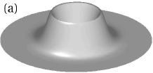
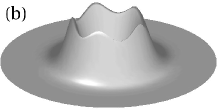
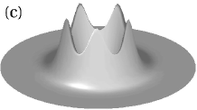
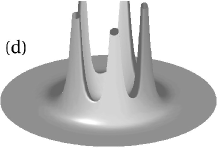
Figure 1: A typical numerical simulation of a vortex solution to the NLS showing MI. The vortex shown is of charge $m=2$ perturbed with mode $K=5$ starting with a perturbation amplitude of $\epsilon=0.001$. (a) $t=0$, (b) $t=8$, (c) $t=10$, and (d) $t=12$.

To predict the actual exponential growth rates for the perturbation of each mode from the eigenvalues, the time rescaling of Eq. (13) needs to be taken into account, in which case the growth rates (in terms of $K_{\mbox{\scriptsize crit}}$) are:

$$\lambda_{\pm}=\pm\frac{C_{3}}{C_{1}}\sqrt{K^{2}\left(K_{\mbox{\scriptsize crit}}^{2}-K^{2}\right)}.$$ (23)

4 Variational Approach

Explicit solutions for two dimensional steady-state vortices of the NLS are not available. Therefore, in order to find a tractable, approximate, solution, we use a variational approach (VA) to get a reasonable ansatz, and then use that ansatz as an initial condition to a nonlinear equation optimization routine which finds the numerically ‘exact’ steady-state profile, $f(r)$. The VA-inferred seed may also be of value as an initial guess to other numerical techniques that have been previously used to obtain such vortices, including shooting methods [15] or Newton-type, fixed point schemes [16]. The modified Gauss-Newton scheme presented below is intended as an alternative to the former ones.

To perform the VA, we use the technique described in Ref. [18]. We insert a vortex ansatz with variable parameters into the Lagrangian of the NLS, and use the Euler-Lagrange equations to find the ‘best’ values for the parameters. We start with a general, separable, steady-state solution:

$$\Psi(r,\theta,t)=f(r)e^{i(m\theta+\Omega t)},$$ (24)

where $f(r)$ is the steady-state radial profile which we want to find. Inserting this solution into the Lagrangian density of the NLS yields:

$$L=2\pi\left(\Omega\,C_{1}+m^{2}\,C_{3}+C_{2}-\frac{1}{2}\,C_{4}\right),$$ (25)

where we have now explicitly set $s=+1$ and the $C$-constants are the same as in Eq. (9).

We use a one-dimensional soliton sech ansatz similar to that used in Ref. [28]:

$$f(r)=\sqrt{B}\,\mbox{sech}\left(\sqrt{\frac{B}{2}}(r-r_{c})\right),$$ (26)

with parameters $B$ and $r_{c}$ corresponding, respectively, to the amplitude and location of the ring induced by the vortex. Now assuming $r_{c}$ to be large, we can approximate the $C$-constants as follows:

$$C_{1} = \int_{0}^{\infty}\!B\,\mbox{sech}^{2}\left(F\right)r\,dr=2\,\mbox{ln}\left(1+E\right)\approx r_{c}\,\sqrt{8B},$$ (27)

$$C_{2} = \int_{0}^{\infty}\!\frac{B^{2}}{2}\,\mbox{sech}^{2}\left(F\right)\,\mbox{tanh}^{2}\left(F\right)r\,dr$$

$$= \frac{B\left[\ln\left(1+E\right)\left(E^{2}+E+1\right)+2\,E\right]}{3\left(1+E\right)^{2}}\approx\frac{\sqrt{2}}{3}r_{c}\,B^{3/2}.$$

$$C_{4} = \int_{0}^{\infty}\!B^{2}\,\mbox{sech}^{4}\left(F\right)r\,dr=4\,C_{2}\approx\frac{4\sqrt{2}}{3}r_{c}\,B^{3/2},$$ (29)

where $E\equiv e^{\sqrt{2B}r_{c}}$ and $F\equiv\sqrt{\frac{B}{2}}(r-r_{c})$. The $C_{3}$ integral does not converge due to the singularity at $r=0$. However, since we assume $r_{c}$ to be large, the $r$ in the integrand can be viewed as a constant (which we choose to be the center of the sech, i.e. $r_{c}$) and so we have:

$$C_{3} = \int_{0}^{\infty}\!\frac{1}{r}\,B\,\mbox{sech}^{2}\left(F\right)\,dr\approx\frac{1}{r_{c}}\int_{0}^{\infty}\!B\,\mbox{sech}^{2}\left(F\right)\,dr$$ (30)

$$= \frac{\sqrt{8B}}{r_{c}}\,\frac{e^{\sqrt{2B}r_{c}}}{(1+E)}\approx\frac{\sqrt{8B}}{r_{c}},$$

Using these approximations, we obtain:

$$L=\frac{2\pi}{3}\,\sqrt{2B}\,r_{c}\left(6\,\Omega+6\,\frac{m^{2}}{r_{c}^{2}}-B\right).$$

The Euler-Lagrange equations:

$$\frac{\partial L}{\partial B}=0,\qquad\frac{\partial L}{\partial r_{c}}=0,$$

lead us to the solution:

$$B=3\Omega,\qquad r_{c}=\sqrt{\frac{2m^{2}}{\Omega}},$$ (31)

and so our VA ansatz is:

$$f(r)=\sqrt{3\,\Omega}\,\mbox{sech}\left[\sqrt{\frac{3\,\Omega}{2}}\left(r-\sqrt{\frac{2m^{2}}{\Omega}}\right)\right].$$ (32)

Despite the obvious problem with this solution at $r=0$ (where $f(0)$ should identically be equal to $0$), it captures the shape and position of the numerically ‘exact’ solution very well (see Fig. 2). Also for higher $m$, its value at $r=0$ becomes very close to zero.

Using the VA ansatz with the asymptotic approximations of Eqs. (27)–(30), we can calculate analytical expressions for the exponential growth rates and critical modes of the MI:

$$K_{\mbox{\scriptsize crit}}^{\mbox{\scriptsize va}} =\pm 2\sqrt{2}m,$$ (33)

$$\lambda^{\mbox{\scriptsize va}} =K\Omega\,\frac{\sqrt{8m^{2}-K^{2}}}{2m^{2}}.$$

The advantage of the above formula is that, although approximate, they describe in simple terms the MI experienced by the vortex. Also, it should be noted that this analytical prediction becomes more accurate for higher order vortices as the VA is able to closely match the actual solution as depicted in Fig. 2.

5 Numerical Results

5.1 Numerical Optimization

To refine the ansatz profile into a numerically ‘exact’ solution, we implement a nonlinear optimization scheme based on a modified Gauss-Newton scheme [29]. First, we insert the following separable steady-state solution into Eq. (3):

$$\Psi(r,\theta,t)=f(r)\,e^{i(m\theta+\Omega t)},$$ (34)

which produces an ordinary differential equation for $f(r)$ which can be discretized as:

$$F_{i}(f_{i}(r_{i}))=-\left(\Omega+\frac{m^{2}}{r_{i}^{2}}\right)f_{i}+D(f_{i})+f_{i}^{3}=0,$$ (35)

where

$$D(f_{i})=\frac{1}{r_{i}}\frac{1}{\Delta r}\left(r_{i+\frac{1}{2}}\frac{f_{i+1}-f_{i}}{\Delta r}-r_{i-\frac{1}{2}}\frac{f_{i}-f_{i-1}}{\Delta r}\right).$$ (36)

We now want a profile, $\vec{f}_{0}$, which optimizes $\vec{F}$ towards the specific value $\vec{0}$. To do this we iterate the trial profile using:

$$\vec{f}_{k+1}=\vec{f}_{k}+\alpha_{k}\vec{p}_{k},$$

where the step length $\alpha_{k}$, is found by:

$$\min_{\alpha>0}M(\vec{f}_{k}+\alpha\vec{p}_{k})\rightarrow\alpha_{k},$$

and where $M(\vec{f}_{k})$ is the merit function defined by:

$$M(\vec{f})=\frac{1}{2}\sum_{i=1}^{n}\,(F_{i}(\vec{f}))^{2}.$$ (37)

The step direction, $\vec{p}_{k}$ is found using a modified Gauss-Newton (GN) formulation:

$$\vec{p}_{k}=-(J_{k}^{T}J_{k}+\Lambda_{k}I)^{-1}J_{k}^{T}\vec{F}(f_{k}),$$ (38)

where $\Lambda_{k}$ is called the forcing term, which ensures that the step is always defined, even near non-zero roots of $M$. The forcing term is manually set to values which produce desired results for our problem ($\Lambda_{k}=0.001$). Some sample profiles for various charges are shown in Fig. 2, where we can see the very good agreement between VA and the numerically ‘exact’ solution, especially for higher charges.

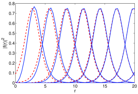
Figure 2: (Color online) Comparison between the VA ansatz (dashed/red lines) and the numerically ‘exact’ solution (solid/blue lines) for charges $m=1,...,7$ (curves left to right). We notice that the VA captures the numerically ‘exact’ solution very well as $m$ increases.

The apparent convergence of the VA ansatz with the GN refined profile as $|m|$ increases can be very useful. For very large $|m|$, the GN computation using a high enough resolution to avoid numerical errors can become very computationally expensive. Therefore, the analytic stability predictions of the VA [see Eq. (33)] can be used for predictions without the need to run numerical computations at all. Even for low charges, the VA ansatz accurately describes the radius and maximum intensity of the vortex.

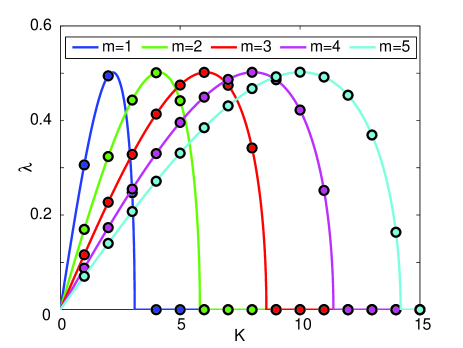
Figure 3: (Color online) Numerical predictions of growth rates of perturbations of azimuthal modes ($K$) for vortices with $\Omega=0.25$ and charges $m=1,...,5$ (left to right) using the numerical routine described in Sec. 5 to converge the VA ansatz into a numerically ‘exact’ solution. The predictions are made numerically integrating the constants of Eq. (9). We see that for each $m$, after the critical mode, the growth rate predictions for each $K$ become $0$ indicating that the perturbations after the critical mode are stable.

5.2 Two-dimensional Simulations

We now compare our predictions for the MI growth rates for vortex charges $m=1,...,5$ using Eq. (23) to numerical results, see Fig. 3. To verify our predictions we use a polar-grid finite-difference scheme where we treat the time derivative separately from the spatial derivatives. For the time derivatives, we use the fourth order Runge-Kutta method. For the spatial derivatives we use a second-order central difference scheme:

$$\nabla^{2}\Psi_{i,j}=D(\Psi_{i})+\frac{1}{r_{i}^{2}}\frac{\Psi_{i,j+1}-2\Psi_{i,j}+\Psi_{i,j-1}}{\Delta\theta^{2}}.$$

For our simulations we use $\Omega=0.25$, $\Delta r=0.35$, $\Delta\theta={2\pi}/{80}$, $\Delta t=0.0005$, with a length of the simulation $t_{\mbox{\scriptsize max}}=15$, and a perturbation amplitude $\epsilon=0.00001$.

Using this scheme, along with Dirichlet boundary conditions, yields the results in Figs. 4 and 5 for $m=2$ and $m=3$, respectively. The growth rates are calculated by recording the maximum and minimum of the modulus squared of the crest of the vortex, and computing the average growth rate of the perturbation growth.

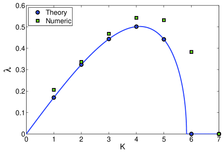
Figure 4: (Color online) Average growth rates from full two-dimensional simulation of vortices of charge $m=2$ perturbed with modes $K=1,...,7$ compared to numerical predictions. The predicted growth rates are shown in blue circles, while the green squares represent the computed growth rates from the full simulation.

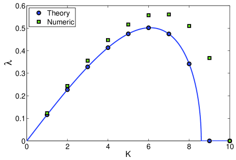
Figure 5: (Color online) Same as in Fig. 4 for $m=3$.

Overall, we see that our numerical simulations yield growth rates that are close to those predicted, but typically slightly higher, with an error on the order of $10\%$ for modes far from $K_{\mbox{\scriptsize crit}}$. For modes close to $K_{\mbox{\scriptsize crit}}$, we observe higher error. Also, for $m=2$ and $m=3$, the predicted $K_{\mbox{\scriptsize crit}}$ is one mode off.

Through one-dimensional simulations, as well as numerical error analysis, we have accounted for much of this error. It is observed that for modes closer to $K_{\mbox{\scriptsize crit}}$, the simulations are very sensitive to resolution. By increasing the resolution to very high levels, the discrepancy in the one-dimensional runs were virtually eliminated. Such high resolutions were not used for the 2D simulations because the simulations become very computationally expensive. Additionally, due to the singularities in the $C$-constant integrals, the numerical predictions derived from them also induce slight errors.

Another source of the discrepancy between our predictions and the simulations (especially the fact that our critical mode prediction is off by one) is that the assumption of separability used in Eq. (7) is not exact, but rather a good approximation. This can be seen by plotting the 2D eigenvectors of the steady-state vortices as seen in Fig. 6.

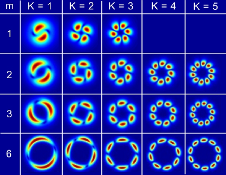
Figure 6: (Color online) Depiction of the modulus squared of numerically derived unstable eigenmodes of vortices in the 2D focusing NLS of charges $m=1,2,3,$ and $6$ for modes $K=1,...,5$ (the vortex of charge $m=1$ does not have unstable modes past $K=3$). It is obvious from the panels that the eigenmodes are not completely separable into radial and azimuthal parts as assumed in Eq. (7), but can be reasonably approximated by such a separable solution. We also see that for higher charges and higher mode numbers, the eigenmodes appear to become more separable, and thus the approximation of a separable solution becomes more accurate.

We see that for low vortex charges, and small mode perturbations, the eigenvectors are clearly non-separable into radial and azimuthal parts. As one increases the charge and/or the mode being perturbed, the eigenvector becomes more separable. Since our simulations were done on vortices of low charge, some discrepancy due to the assumption of Eq. (7) is to be expected [30].

Finally, we note in passing that our approach is somewhat complementary to the theoretical approach of Ref. [15], while the combination of both is in some sense tantamount to the theoretical analog of what is found numerically in Refs. [15, 16]. In Ref. [15], the so-called Vakhitov-Kolokolov criterion was considered which is implicitly connected to the $K=0$ perturbation mode and the instability along that eigendirection leads to collapse. On the other hand, here we examine the modulational-type instability of higher $K$ modes which initiates the unstable dynamics by breakup of the azimuthal symmetry (and may, however, eventually lead to collapse in conjunction with the $K=0$ mode, as shown in Fig. 1).

6 Nonlocal Nonlinearity

Here we briefly describe one of the possible extensions to the theory, that of incorporating nonlocal interactions. Such interactions correspond to various physical systems, such as dipole-dipole interactions in a BEC of degenerate dipolar atoms [31], and nonlinear crystals whose nonlinear refractive index changes due to the intensity of the light present (determined by a transport process such as heat conduction) [32]. As we will show, the nonlocality of the nonlinearity will induce a stabilizing effect on the modulational stability of vortices. Other interesting effects of the nonlocality of the nonlinearity include: changing, under appropriate circumstances, the character of interaction of dark solitons from repulsive to attractive [33]; changing the interaction strength between solitons [34]; and stabilization of dipole solitons [35] or 2D ring vortices such as the ones considered herein [36]. We note that prior work has demonstrated that for the case of nonlocal $\chi^{(3)}$ nonlinearity, all three dimensional spatiotemporal solitons with vorticity are unstable [37].

For nonlocal interactions, the NLS can be altered to have a nonlocal nonlinearity [32]

$$i\Psi_{t}+\nabla^{2}\Psi+sN\!\left(\left|\Psi\right|^{2}\right)\!\Psi=0,$$ (39)

where the nonlocal nonlinearity takes the form of a convolution integral:

$$N=\int_{0}^{2\pi}\!\!\int_{0}^{\infty}\!V\!\left(r^{\prime}-r,\theta^{\prime}-\theta\right)\left|\Psi\!\left(r^{\prime},\theta^{\prime},t\right)\right|^{2}r^{\prime}\,dr^{\prime}\,d\theta^{\prime},$$

and where $V$, the nonlocal response function, is taken to be a Gaussian (which appears in relation to the nonlinear crystal heat diffusion nonlocality [32]):

$$V\!\left(r^{\prime}-r,\theta^{\prime}-\theta\right) = \frac{1}{\pi\sigma^{2}}\exp\!\left(-\frac{|\overrightarrow{r}^{\prime}-\overrightarrow{r}|^{2}}{\sigma^{2}}\right),$$

where $\overrightarrow{r}\!=\!(r\cos\theta,r\sin\theta)$ and $\overrightarrow{r}^{\prime}\!=\!(r^{\prime}\cos\theta^{\prime},r^{\prime}\sin\theta^{\prime})$. Formulating the Lagrangian density of Eq. (39) yields:

$$\mathcal{L}=\frac{i}{2}\left(\Psi\Psi_{t}^{*}-\Psi^{*}\Psi_{t}\right)+\left|\Psi_{r}+\frac{1}{r}\Psi_{\theta}\right|^{2}-\frac{s}{2}|\Psi|^{2}N(|\Psi|^{2})\left.\right.,$$

which, by the same method as in Sec. 2, yields the following azimuthal equation of motion:

$$i\,C_{1}A_{t}=C_{2}A-C_{3}A_{\theta\theta}-s\,C(\theta,t)A,$$ (40)

where $C$ is defined as:

$$C(\theta,t) = \int_{0}^{2\pi}\!\!\!\int_{0}^{\infty}\!\!\!\int_{0}^{\infty}\!V\!\left(r^{\prime}-r,\theta^{\prime}-\theta\right)\,\times$$

$$f(r)^{2}f(r^{\prime})^{2}|A(\theta^{\prime},t)|^{2}rr^{\prime}\,dr\,dr^{\prime}\,d\theta^{\prime}.$$

Note that the new, nonlocal, azimuthal NLS (40) is the same as in the local case [see Eq. (11)] where the (local) $C_{4}$ integral has been replaced by the (nonlocal) convolution $C$ integral (6).

We use the same stability analysis technique as in Sec. 2, with a slight alteration. We notice that if we define:

$$R(\theta^{\prime}-\theta) = \int_{0}^{\infty}\!\!\int_{0}^{\infty}\!V\!\left(r^{\prime}-r,\theta^{\prime}-\theta\right)\,f(r)^{2}f(r^{\prime})^{2}\,rr^{\prime}\,dr\,dr^{\prime},$$

then $C$ is now a convolution term as follows:

$$C(\theta,t)=\int_{0}^{2\pi}\!R(\theta^{\prime}-\theta)|A(\theta^{\prime},t)|^{2}\,d\theta^{\prime}=R*|A|^{2}.$$

Inserting this into Eq. (40), and using the same rescalings as in Eqs. (12) and (13), yields

$$iA_{t}=-A_{\theta\theta}-\frac{s}{C_{3}}A(R*|A|^{2}).$$

Now, we perform a stability analysis identical to that of Sec. 3, but along with the transforms of $\hat{u}$ and $\hat{v}$, we also add:

$$\hat{R}(K)=\int_{0}^{2\pi}R(\theta)e^{iK\theta},$$

in which case the convolution term becomes a product ($A\hat{R}$), and we get:

$$\lambda_{\pm}=\pm\frac{C_{3}}{C_{1}}\sqrt{K^{2}\left(2s\frac{\hat{R}(K)}{C_{3}}-K^{2}\right)},$$

and, therefore, the critical mode is:

$$K_{\mbox{\scriptsize crit}}=\pm\sqrt{2s\frac{\hat{R}(K)}{C_{3}}},$$

which has the same form as the local nonlinearity case after replacing $C_{4}$ with $\hat{R}(K)$. We see that depending on the nonlocal response function, $K_{\mbox{\scriptsize crit}}$ can be damped, and if $\hat{R}(K)<\left|\frac{C_{3}}{2s}\right|$ then $K_{\mbox{\scriptsize crit}}<1$ and all modes become stable. Therefore, we see that one could have a vortex in the focusing NLS with a nonlocal nonlinearity which would be modulationally stable. In fact, this modulational stability (as well as the stability against collapse) of the focusing ring vortices of the nonlocal NLS equation has been confirmed in the work of Ref. [36] and is a feature that could have practical applications, such as data storage and communications using light vortices in Kerr optical media [38].

7 Conclusions

We have formulated a methodology for studying azimuthal modulational instability of vortices in the two-dimensional nonlinear Schrödinger (NLS) equation which can be extended to incorporate any additional terms in the NLS as long as they have a Lagrangian representation. (This expandability of the method adds greatly to its usefulness and broad relevance). The method relies on approximating a vortex solution as being separable into its radial and azimuthal parts, and using the Lagrangian functional of the NLS to obtain a quasi-one-dimensional equation of motion for the azimuthal direction. A stability analysis on modulational perturbations of the equation, leads to predictions of growth rates for each perturbed mode, and of the critical mode. After obtaining a steady-state vortex solution using a variational ansatz along with a nonlinear optimization routine, we ran numerical simulations of the NLS, perturbing individual modes and recording their growth rates to confirm the predictions.

One key result that should not be overlooked is that of the usefulness of the variational ansatz of the vortex profiles that we derived. Since this profile seems to converge to the numerically exact solution as the vortex charge becomes large, experimenters can use it to make simple yet accurate predictions of the vortex radius and intensity given experimental parameters. Furthermore, it can be used as in Ref. [15], in both local and nonlocal settings to yield an approximate threshold for collapse dynamics.

We have also shown theoretical predictions of modulational instability of vortices which exhibit a nonlocal response by extending the NLS to incorporate a nonlocal nonlinearity. The results illustrate that nonlocality can damp, or completely eliminate, the modulational instability, potentially leading to the complete stabilization of the nonlocal vortices, as shown numerically, e.g., in Ref. [36].

References

- [1] A.C. Scott. Nonlinear Science: Emergence & Dynamics of coherent structures (2nd. ed.), OUP, Oxford, 2003.
- [2] C.J. Pethick and H. Smith, Bose-Einstein condensation in dilute gases, Cambridge University Press (Cambridge, 2002); L.P. Pitaevskii and S. Stringari, Bose-Einstein Condensation, Oxford University Press (Oxford, 2003).
- [3] P.G. Kevrekidis, D.J. Frantzeskakis, and R. Carretero-González (eds). Emergent Nonlinear Phenomena in Bose-Einstein Condensates: Theory and Experiment. Springer Series on Atomic, Optical, and Plasma Physics, Vol. 45, 2008.
- [4] Yu.S. Kivshar and G.P. Agrawal, Optical solitons: from fibers to photonic crystals, Academic Press (San Diego, 2003).
- [5] C.A. Sackett, J.M. Gerton, M. Welling, and R.G. Hulet, Phys. Rev. Lett. 82, 876 (1999).
- [6] J.M. Gerton, D. Strekalov, I. Prodan, and R.G. Hulet, Nature 408, 692 (2001).
- [7] E.A. Donley, N.R. Claussen, S.L. Cornish, J.L. Roberts, E.A. Cornell, and C.E. Wieman, Nature 412, 295 (2001).
- [8] M. Ueda and H. Saito. J. Phys. Soc. Jap. 72, 127 (2003).
- [9] R. Carretero-González, D.J. Frantzeskakis and P.G. Kevrekidis. Nonlinearity 21 R139 (2008).
- [10] L. Salasnich, A. Parola and L. Reatto, Phys. Rev. A 65, 043614 (2002).
- [11] A. Muñoz Mateo and V. Delgado Phys. Rev. A 77, 013617 (2008).
- [12] D. E. Pelinovsky, Y. A. Stepanyants and Y. S. Kivshar. Phys. Rev. E 51, 5016 (1995).
- [13] V.I. Kruglov, Yu.A. Logvin and V.M. Volkov, J. Mod. Opt. 39, 2277 (1992).
- [14] M.S. Bigelow, Q.-H. Park, and R.W. Boyd, Phys. Rev. E 66, 046631 (2002).
- [15] L.D. Carr and C.W. Clark, Phys. Rev. Lett. 97, 010403 (2006); Phys. Rev. A 74, 043613 (2006).
- [16] G. Herring, L. D. Carr, R. Carretero-González, P. G. Kevrekidis, and D. J. Frantzeskakis, Phys. Rev. A, 77, 023625 (2008).
- [17] W.Z. Królikowski, O. Bang, N.L. Nikolov, D. Neshev, J. Wyller, J.J. Rasmussen and D. Edmundsson, J. Opt. B 6, S288 (2004).
- [18] B. Malomed. Progress in Optics, 43, 71 (2002).
- [19] A. Hasegawa, Solitons in Optical Communications, Clarendon Press (Oxford, NY 1995).
- [20] W. Królikowski, O. Bang, J. J. Rasmussen and J. Wyller. Phys. Rev. E, 64, 016612 (2001).
- [21] V.L. Ginzburg and L.P. Pitaevskii, Zh. Eksp. Teor. Fiz. 34, 1240 (1958) [Sov. Phys. JETP 34, 858 (1958)].
- [22] H. Pu, C. K. Law, J. H. Eberly, and N. P. Bigelow, Phys. Rev. A, 59, 1533 (1999).
- [23] Y. Kawaguchi, T. Ohmi, Phys. Rev. A 70, 043610 (2004).
- [24] M. Okano, H. Yasuda, K. Kasa, M. Kumakura, and Y. Takahashi, J. Low. Temp. Phys. 148 447 (2007);
- [25] T. Isoshima, M. Okano, H. Yasuda, K. Kasa, J. A. M. Huhtamaki, M. Kumakura, and Y. Takahashi, Phys. Rev. Lett. 99, 200403 (2007).
- [26] D. Mihalache, D. Mazilu, B.A. Malomed, and F. Lederer, Phys. Rev. A 73, 043615 (2006).
- [27] T.J. Alexander and L. Bergé, Phys. Rev. E 65, 026611 (2002).
- [28] V. V. Afanasjev. Phys. Rev. E, 52, 3153 (1995).
- [29] J. Nocedal and S. J. Wright. Numerical Optimization. Springer, New York, New York, 2 edition, 2006.
- [30] R.M. Caplan. MS Thesis, San Diego State University (2008).
- [31] V. M. Lashkin. Phys. Rev. A, 75, 043607 (2007).
- [32] J. Wyller, W. Królikowski, O. Bang and J. J. Rasmussen. Phys. Rev. E, 66, 066615 (2002).
- [33] A. Dreischuh, D. N. Neshev, D. E. Petersen, O. Bang, and Królikowski, Phys. Rev. Lett., 96, 043901 (2006).
- [34] F. Ye, Y. V. Kartashov, and Ll. Torner, Phys. Rev. A 76, 033812 (2007).
- [35] F. Ye, Y. V. Kartashov, and Ll. Torner, Phys. Rev. A 77, 043821 (2008).
- [36] D. Briedis, D. Petersen, D. Edmundson, W. Królikowski, and O. Bang, Opt. Express 13, 435-443 (2005)
- [37] D. Mihalache, D. Mazilu, F. Lederer, B.A. Malomed, Y.V. Kartashov, L.-C. Crasovan, and L. Torner, Phys. Rev. E 73, 025601 (2006).
- [38] Y. S. Kivshar and E. A. Ostrovskaya. Optics and Photonics News, 12, 24 (2001).