Role of the attractive intersite interaction in the extended Hubbard model

Abstract

We consider the extended Hubbard model in the atomic limit on a Bethe lattice with coordination number $z$. By using the equations of motion formalism, the model is exactly solved for both attractive and repulsive intersite potential $V$. By focusing on the case of negative $V$, i.e., attractive intersite interaction, we study the phase diagram at finite temperature and find, for various values of the filling and of the on-site coupling $U$, a phase transition towards a state with phase separation. We determine the critical temperature as a function of the relevant parameters, $U/|V|$, $n$ and $z$ and we find a reentrant behavior in the plane ($U/|V|$,$T$). Finally, several thermodynamic properties are investigated near criticality.

1 Introduction

Understanding the effects of competing interactions and the corresponding quantum phase transitions in models of strongly correlated electron systems is a crucial problem in condensed matter physics. A thorough comprehension could shed new light on the behavior of new classes of novel materials, ranging from inorganic chain compounds and conducting polymers to organic and high temperature superconductors. In all such systems, long-ranged Coulomb interactions play an essential role, as it has been pointed out in Ref. imada , where it was shown that the simple Hubbard model does not offer a model for the superconductivity in the right order of amplitude. Similarly, Frölich and Coulomb long-ranged interactions have been recognized to play an essential role in a realistic multi-polaron model of high-$T_{c}$ superconductivity alexandrov3 .

Here, we study the so-called extended Hubbard model (EHM) exhub1 , where a nearest-neighbor interaction $V$ is added to the original Hubbard Hamiltonian, containing only an on-site interaction $U$. The intersite interaction can somehow mime longer-ranged Coulomb interactions. In various applications of the model, the parameters $U$ and $V$ can represent the effective interaction couplings taking into account also other interactions (for instance with phonons). Therefore we assume that $U$ and $V$ could take positive as well as negative values. The EHM has been deeply investigated by means of various analytical techniques. In particular, g-ology investigations exhub3 as well as renormalization group exhub4 and bosonization exhub5 analysis have been successfully carried out in the weak coupling regime, while exact diagonalization calculations exhub6 and quantum Monte Carlo simulations exhub7 have been used to study the intermediate and strong coupling regimes exhub8 . The cases of half filling ($n=1$) exhub7 and quarter filling ($n=0.5$) exhub9 have been deeply investigated in order to establish the boundary line between spin-density wave and charge-density wave phases, as well as existence of an intermediate bond-order wave phase. More recently several systematic studies of the phase diagram of the one-dimensional extended Hubbard model as a function of all the three parameters $n$, $U$, $V$ have been performed as well exhub10 , revealing a very rich structure due to the presence of multiple first and second order phase transitions, critical points and interesting reentrant behaviors exhub11 . The relation with the experimental findings relative to some manganese compounds exhub12 has been investigated in detail together with the possibility of improving the description of cuprates with respect to the simple Hubbard model exhub11 . However, despite of the above results, such a general case still lacks a detailed study.

In order to overcome the difficulties shown by the EHM and to investigate charge ordering in interacting electron systems, one may consider a minimal model, allowing one to capture all the relevant phenomenology while being exactly solved. That is, one can consider the very narrow band limit, where $t_{ij}\ll U,V$; for simplicity the classical limit $t_{ij}=0$ can be taken. In this way one is led to the extended Hubbard model in the atomic limit (AL-EHM), which is one of the simplest models apt to describe charge ordering in interacting electron systems. The charge ordering has attracted much attention after the discovery of charge-density waves in high temperature superconductors and since then the problem of competition and coexistence of this kind of ordering and other orderings has been widely investigated ch1 . Charge ordering is in fact accompanied by metal-insulator transitions through the growth of charge-order parameter and the opening of gaps at the Fermi surface. Furthermore, phenomena such as colossal magnetoresistance in perovskite-type manganese oxides are observed immediately when the charge order melts ch2 ; ch3 . Recently charge orderings and charge-density waves have been widely observed in transition metal compounds ch4 and also in organic conductors ch5 . It is worth noticing that the observed changes in transport, optical, dielectric and magnetic properties at or near charge-order transitions have spurred a lot of interest on the problem of their control through the charge-order transitions. Thus, in this context, a deeper understanding of the nature of charge-order transitions could be relevant as well as of the whole structure of the phase diagrams. Another aspect which is very interesting and deserves further investigations is the phase separation phenomenon phasesep1 ; pawlowski1 ; phasesep1a ; it has been investigated in some detail in the AL-EHM context by means of Monte Carlo simulations and Hartree-Fock approximation in Ref. phasesep2 and the results have been compared with the experimental ones obtained for the organic conductor $(DI-DCNQI)_{2}Ag$ phasesep3 . The phase separation phenomenon is characterized by a ground state macroscopically inhomogeneous with different spatial regions with different average charge densities. Typically, it occurs for attractive on-site and intersite interactions, so that the electrons cluster together in order to gain the maximum negative potential energy. In the extended Hubbard model, two types of phase separated configurations are possible: a cluster of singly occupied sites or a cluster of doubly occupied sites, as shown in Fig. 1.

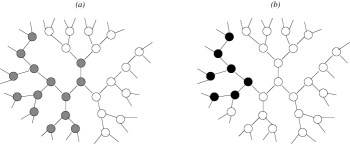
Figure 1: Distribution of the particles along the Bethe lattice at $n=0.5$ and $T=0$: ($a$) $V<0$ and $U\gtrapprox 2V$; ($b$) $V<0$ and $U\lessapprox 2V$. White, grey and black squares denote empty, arbitrary spin singly occupied and double occupied sites, respectively.

A cluster of doubly occupied sites is favored when the on-site and intersite interactions are both attractive, whereas cartoon ($b$) would correspond to large positive $U$ and negative $V$.

The critical behavior of the AL-EHM has been studied by many authors, mainly in the one dimensional case sf1 ; sf2 ; sf3 ; sf4 ; sf5 ; sf6 ; sf7 ; sf8 ; sf9 ; 2 , and a staggered charge order has been found irrespectively of the method of analysis. Very recently, a comprehensive and systematic analysis of the one dimensional AL-EHM has been carried out both at $T=0$ and finite temperature in the whole parameters space and various types of long-range charge ordered states have been observed mancini2 . A study of the two-dimensional version of the model has been performed pawlowski1 ; pawlowski , and very recently the same model on a Bethe lattice with general coordination number $z$ has been investigated 4 .

The study of the extended Hubbard model with attractive as well as repulsive on-site and intersite interactions could also shed new light on the properties of systems of ultracold fermionic atoms loaded in optical lattices, such as fermionic superfluid properties in a two dimensional lattice volcko , and the possibility of the supersolid state jaksch .

In this paper we study the AL-EHM on a Bethe lattice with coordination number $z$ within the equations of motion framework 2 ; 1 ; 3 . This formalism allows us to exactly solve the model. By focusing on the case of attractive $V$, we study the phase diagram at finite temperature $T$ for different values of the filling and the coupling $U/\left|V\right|$. By varying the temperature, we find a region of negative compressibility, hinting at a transition from a thermodynamically stable to an unstable phase characterized by phase separation. The critical temperature, function of the external parameters $U/\left|V\right|$, $n$ and $z$, shows a reentrant behavior in the plane $\left(U/\left|V\right|,T\right)$ at half filling ($n=1$). Although thermodynamically unstable, the study of the $T<T_{c}$ phase allows us to determine the critical value of the on-site interaction $U_{c}$ separating the formation of clusters of singly and doubly occupied sites.

The plan of the paper is as follows: in Sec. 2, we briefly review the equations of motion method for the extended Hubbard model in the atomic limit on a Bethe lattice with coordination number $z$ and compute the Green’s and correlation functions. We find that they crucially depend only on two parameters, which can be self-consistently computed allowing us to determine all the local properties of the system in the case of general filling $n$. In Sec. 3 we derive the phase diagram in the planes ($n,T$) and ($U,T$) for a Bethe lattice with coordination number $z=3$, and we show the behavior of the relevant thermodynamic quantities. Finally, Sec. 4 is devoted to our concluding remarks.

2 The general model

The extended Hubbard Hamiltonian in the narrow-band limit on a Bethe lattice with coordination number $z$ and nearest-neighbor interactions is given by:

$$H=-\mu n(0)+UD(0)+\sum\limits_{p=1}^{z}H^{(p)}.$$ (1)

Here $H^{(p)}$ represents the Hamiltonian of the $p$-th sub-tree rooted at the central site (0):

$$H^{(p)}=-\mu n(p)+UD(p)+Vn(0)n(p)+\sum\limits_{m=1}^{z-1}H^{(p,m)},$$ (2)

where $p$ ($p=1,\ldots,z$) are the nearest neighbors of the site (0), also termed the first shell. In turn, $H^{(p,m)}$ describes the $m$-th sub-tree rooted at the site $(p)$, and so on to infinity. $U$ and $V$ are the strengths of the local and intersite interactions, $\mu$ is the chemical potential, $n(i)=n_{\uparrow}(i)+n_{\downarrow}(i)$ and $D(i)=n_{\uparrow}(i)n_{\downarrow}(i)=n\left(i\right)\left[n\left(i\right)-1\right]/2$ are the charge density and double occupancy operators at a general site $i$ . As usual, $n_{\sigma}(i)=c_{\sigma}^{{\dagger}}(i)c_{\sigma}(i)$ with $\sigma=\left\{{\uparrow,\downarrow}\right\}$ and $c_{\sigma}(i)$ ($c_{\sigma}^{{\dagger}}(i))$ is the fermionic annihilation (creation) operator of an electron of spin $\sigma$ at site $i$, satisfying canonical anticommutation relations. We adopt the Heisenberg picture $i=\left(\mathbf{i},t\right)$, and we use the spinorial notation for the fermionic fields.

The exact solution of the model can be obtained by using the equations of motion approach in the context of the composite operator method 5 . Following this line, the main point is the choice of the field operators. A convenient operatorial basis is given by the Hubbard operators, $\xi(i)=[n(i)-1]c(i)$ and $\eta(i)=n(i)c(i)$, which satisfy the equations of motion:

$$\begin{split}i\frac{\partial}{\partial t}\xi(i)&=-\mu\xi(i)+zV\xi(i)n^{\alpha}(i),\\ i\frac{\partial}{\partial t}\eta(i)&=(U-\mu)\eta(i)+zV\eta(i)n^{\alpha}(i).\end{split}$$ (3)

Hereafter, for a generic operator $\Phi\left(i\right)$ we shall use the notation $\Phi^{\alpha}(i)=\frac{1}{z}\sum\nolimits_{p=1}^{z}\Phi(i,p)$, $(i,p)$ being the first nearest neighbors of the site $i$. The Heisenberg equations (3) contain the higher-order nonlocal operators $\xi(i)n^{\alpha}(i)$ and $\eta(i)n^{\alpha}(i)$. By taking time derivatives of the latter, higher-order operators are generated. This process may be continued and usually an infinite hierarchy of field operators is created. However, by noting that the number $n(i)$ and the double occupancy $D(i)$ operators satisfy the following algebra

$$\begin{split}n^{p}\left(i\right)&=n\left(i\right)+a_{p}D(i),\\ D^{p}\left(i\right)&=D(i),\\ n^{p}\left(i\right)D(i)&=2D(i)+a_{p}D(i),\end{split}$$ (4)

where $p\geq 1$ and $a_{p}=2^{p}-2$, it is easy to establish the following recursion rule:

$$[n^{\alpha}(i)]^{k}=\sum\limits_{m=1}^{2z}A_{m}^{(k)}[n^{\alpha}(i)]^{m}.$$ (5)

The coefficients $A_{m}^{(k)}$ are rational numbers, satisfying the relations $\sum_{m=1}^{2z}A_{m}^{(k)}=1$ and $A_{m}^{(k)}=\delta_{m,k}$ $(k=1,\cdots,2z)$ 2 . The recursion relation (5) allows one to close the hierarchy of equations of motion. Thus, one may define a new composite field operator 4 :

$$\psi(i)=\left({{\begin{array}[]{*{20}c}{\psi^{(\xi)}(i)}\\ {\psi^{(\eta)}(i)}\\ \end{array}}}\right),$$ (6)

where

$$\psi^{(\xi)}(i)=\left({{\begin{array}[]{*{20}c}{\xi(i)\hfill}\\ {\xi(i)[n^{\alpha}(i)]}\\ \vdots\\ {\xi(i)[n^{\alpha}(i)]^{2z}}\\ \end{array}}}\right),\quad\psi^{(\eta)}(i)=\left({{\begin{array}[]{*{20}c}{\eta(i)}\\ {\eta(i)[n^{\alpha}(i)]}\\ \vdots\\ {\eta(i)[n^{\alpha}(i)]^{2z}}\\ \end{array}}}\right)$$ (7)

satisfy the equations of motion

$$\begin{split}i\frac{\partial}{\partial t}\psi^{(\xi)}(i)=[\psi^{(\xi)}(i),H]&=\varepsilon^{(\xi)}\psi^{(\xi)}(i)\\ i\frac{\partial}{\partial t}\psi^{(\eta)}(i)=[\psi^{(\eta)}(i),H]&=\varepsilon^{(\eta)}\psi^{(\eta)}(i).\end{split}$$ (8)

Here $\varepsilon^{(\xi)}$ and $\varepsilon^{(\eta)}$ are the energy matrices of rank $(2z+1)\times(2z+1)$ 4 whose eigenvalues are:

$$\begin{split}E_{m}^{(\xi)}&=-\mu+(m-1)V,\\ E_{m}^{(\eta)}&=-\mu+U+(m-1)V,\end{split}$$ (9)

where $m=1,\ldots,(2z+1)$. The model has now been formally solved since one has found a closed set of eigenoperators and eigenvalues allowing one to ascertain exact expressions of the retarded Green’s function (GF)

$$G^{(s)}(t-t^{\prime})=\theta(t-t^{\prime})\langle\{\psi^{(s)}(0,t),{\psi^{s}}^{\dagger}(0,t^{\prime})\}\rangle,$$ (10)

and, consequently, of the correlation function (CF)

$$C^{(s)}(t-t^{\prime})=\langle\psi^{(s)}(0,t){\psi^{(s)}}^{\dagger}(0,t^{\prime})\rangle.$$ (11)

Indeed, by means of the equations of motion (8) one finds 4 :

$$G^{(s)}(\omega)=\sum_{m=1}^{2z+1}\frac{\sigma^{(s,m)}}{\omega-E_{m}^{(s)}+i\delta},$$ (12)

and

$$C^{(s)}(\omega)=\pi\,\sum\limits_{m=1}^{2z+1}\sigma^{(s,n)}T_{m}^{(s)}\,\delta\left({\omega-E_{m}^{(s)}}\right),$$ (13)

where $s=\xi,\eta$, $T_{m}^{(s)}=1+\tanh({\beta E_{m}^{(s)}/2})$, $\beta=1/k_{B}T$ and $E_{m}^{(s)}$ are given in Eq. (9). The spectral density matrices $\sigma_{ab}^{(s,n)}$ can be computed by means of the formula:

$$\sigma_{ab}^{(s,n)}=\Omega_{an}^{(s)}\sum\limits_{c=1}^{2z+1}\left[{\Omega_{nc}^{(s)}}\right]^{-1}I_{cb}^{(s)}.$$ (14)

In Eq. (14), $\Omega^{(s)}$ is the $(2z+1)\times(2z+1)$ matrix whose columns are the eigenvectors of the energy matrix $\varepsilon^{(s)}$ and $I^{(s)}$ is the $(2z+1)\times(2z+1)$ normalization matrix whose elements can be written as 4 : $I_{n,m}^{(\xi)}=\kappa^{(n+m-2)}-\lambda^{(n+m-2)}$, $I_{n,m}^{(\eta)}=\lambda^{(n+m-2)}$. Here the charge correlators $\kappa^{(k)}$ and $\lambda^{(k)}$ are defined as

$$\kappa^{(k)}=\langle{[n^{\alpha}(0)]^{k}}\rangle,\quad\lambda^{(k)}=\frac{1}{2}\langle{n(0)[n^{\alpha}(0)]^{k}}\rangle.$$ (15)

By exploiting the recursion relation (5), it is not difficult to show that also $\kappa^{(k)}$ and $\lambda^{(k)}$ obey to similar recursion relations, limiting their computation to the first $2z$ correlators 4 . However, the knowledge of the GFs and of the CFs, is not fully achieved because they depend on the external parameters $n$, $T$, $U$, $V$, as well as on the internal parameters $\mu$, $\kappa^{(k)}$, $\lambda^{(k)}$ ($k=1,...,2z$). The internal parameters can be self-consistently computed by using algebra constraints and symmetry requirements 4 . Within this scheme, in Ref. 4 it has been shown that the charge correlators $\kappa^{(k)}$ and $\lambda^{(k)}$ can be written as a function of only two parameters, $X_{1}$ and $X_{2}$, in terms of which one may find a solution of the model. $X_{1}$ and $X_{2}$ are parameters of seminal importance since all correlators and fundamental properties of the system under study can be expressed in terms of them. Upon requiring translational invariance, one finds two equations allowing one to determine $X_{1}$ and $X_{2}$ as a function of the chemical potential 4 :

$$\begin{split}X_{1}&=2e^{\beta\mu}(1-X_{1}-dX_{2})(1+aX_{1}+a^{2}X_{2})^{z-1}\\ &+e^{\beta(2\mu-U)}[2+(d-1)X_{1}-2dX_{2}](1+dX_{1}+d^{2}X_{2})^{z-1},\\ X_{2}&=e^{\beta(2\mu-U)}[1+dX_{1}-(2d+1)X_{2}](1+dX_{1}+d^{2}X_{2})^{z-1}\\ &-2e^{\beta\mu}K^{2}X_{2}(1+aX_{1}+a^{2}X_{2})^{z-1}.\end{split}$$ (16)

Here we defined $K=e^{-\beta V}$, $a=(K-1)$ and $d=(K^{2}-1)$. In turn, the chemical potential $\mu$ can be determined by fixing the particle density:

$$\begin{array}[]{c}n=\frac{\left(X_{1}-2X_{2}\right)\left(1+aX_{1}+a^{2}X_{2}\right)+2X_{2}\left(1+dX_{1}+d^{2}X_{2}\right)}{\left(1-X_{1}+X_{2}\right)+\left(X_{1}-2X_{2}\right)\left(1+aX_{1}+a^{2}X_{2}\right)+X_{2}\left(1+dX_{1}+d^{2}X_{2}\right)}.\end{array}$$ (17)

Equations (16) and (17) constitute a system of coupled equations ascertaining the three parameters $\mu$, $X_{1}$ and $X_{2}$ in terms of the external parameters of the model $n$, $U$, $V$, $T$. Once these quantities are known, all local properties of the model can be computed.

3 Results and discussion

According to the sign of the intersite potential $V$, the solutions of the self-consistent equations (16) and (17) can be remarkably different. Here we study the case of attractive nearest neighbor interaction $V$ ($V<0$), allowing the on-site interaction to be both repulsive and attractive. Upon fixing $V=-1$ and taking $|V|=1$ as the unit of energy, we study the equations (16) and (17) for various values of the external parameters $n$, $T$ and $U$, focusing on the simpler case $z=3$. By considering higher coordination numbers, one obtains similar results. In Ref. 4 , upon fixing the chemical potential at the half filling value $\mu=zV+U/2$, we have shown that a phase separation exists only for $V<0$. Since experimentally it is possible to tune the density in a controlled way, by varying the doping, here we fix the particle density $n$: the chemical potential will be determined by the system itself according to the values of the external parameters.

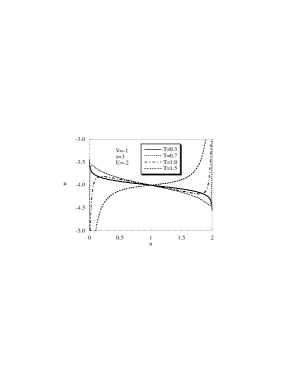
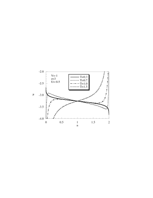
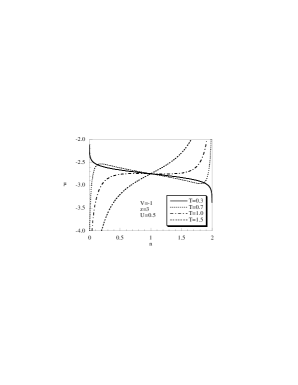
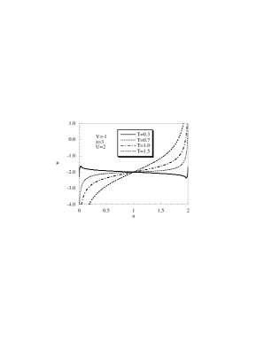
Figure 2: The chemical potential $\mu$ as a function of the particle density $n$ for $V=-1$, $z=3$, $T=0.3$, 0.7, 1, 1.5 and for (a) $U=-2$, (b) $U=-0.5$, (c) $U=0.5$, and (d) $U=2$.

In Figs. 2a-d we plot the chemical potential $\mu$ as a function of the particle density $n$ for both attractive and repulsive on-site interactions, and for several values of the temperature. In the high temperature regime, $\mu$ is always an increasing function of the particle density. By lowering the temperature, one observes that there is a critical value of the temperature below which the chemical potential becomes a decreasing function of $n$ in the interval $n_{1}\leq n\leq n_{2}$. The width of the interval depends on both $T$ and $U$.

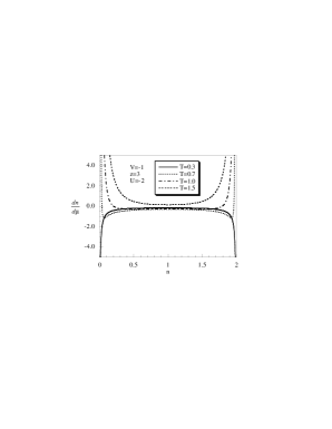
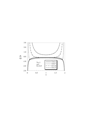
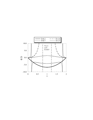
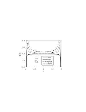
Figure 3: The derivative $dn/d\mu$ as a function of the particle density $n$ for $V=-1$, $z=3$, $T=0.3$, 0.7, 1, 1.5 and for (a) $U=-2$, (b) $U=-0.5$, (c) $U=0.5$, (d) $U=2$.

In Figs. 3 we plot the derivative $dn/d\mu$ as a function of $n$ for the same values of $T$ and $U$ given in Figs. 2. One observes that, at high temperatures, $dn/d\mu$ is a regular function, always positive, for all values of $n$. At low temperatures, $dn/d\mu$ exhibits a divergence at the critical points $n_{1}$ and $n_{2}$, is negative in the interval $n_{1}\leq n\leq n_{2}$, and positive outside. Since the derivative $dn/d\mu$ is proportional to the thermal compressibility $\kappa=1/n^{2}\cdot dn/d\mu$, one immediately infers that $n_{1}\leq n\leq n_{2}$ is a particle density region where the system is thermodynamically unstable. A possible solution to this problem is to abandon the translational invariance assumption made in order to obtain the self-consistent equations (16). Nevertheless, here we are interested only in describing the transition to a phase separated regime, and, thus, we shall not address the problem of finding a thermodynamically stable solution.

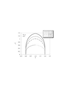
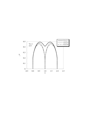
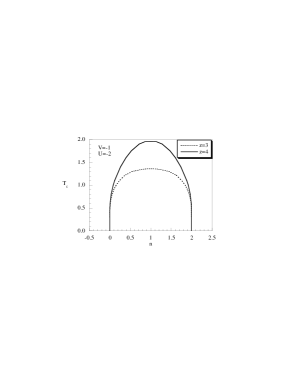
Figure 4: The critical temperature $T_{c}$ as a function of the particle density $n$ for $V=-1$, $z=3$ and for (a) $U=-2$, -0.5, 0.5, 2; (b) $U=2.3$, 2.5, 3. (c) Comparison between the critical temperatures for $z=3$ and $z=4$.

By studying the temperature dependence of $n_{1}$ and $n_{2}$, one can obtain the phase diagram in the plane $(n,T)$. For a fixed value of $n$, there is a critical temperature $T_{c}$ at which the system undergoes a phase transition from a thermodynamically stable phase to an unstable one. Below $T_{c}$ the homogeneous state is not allowed due to a negative compressibility, and a phase separation occurs. In Figs. 4a-b we plot $T_{c}$ as a function of the particle density for several values of $U$. The critical temperature $T_{c}$ and the width of the instability region $\Delta n=n_{2}-n_{1}$ increase by decreasing $U$: an attractive on-site potential will favor phase separation and in particular the clustering of doubly occupied sites. As a function of the particle density, the critical temperature shows a lobe-like behavior: it increases by increasing $n$ up to half filling, where it has a maximum; further augmenting $n$, it decreases vanishing at $n=2$. A different behavior is observed when $U>2\left|V\right|$ (see Fig. 4b): the lobe splits in two parts and $T_{c}$ increases with $n$ up to quarter filling, then decreases with a minimum at half filling. The $n=1$ critical temperature is finite only for $2V<U<U_{c}$, where $U_{c}=2.3V$ for $z=3$. For larger on-site potentials, there is no transition at half filling. For higher coordination number, one notices an increase of the critical temperature, as evidenced in Fig. 4c, where we compare $T_{c}$ at $U=-2$ for $z=3$, 4. A useful representation of the phase diagram is obtained by plotting the phase boundary line in the plane $(T_{c},U)$. In Fig. 5 we plot the critical temperature $T_{c}$ as a function of the on-site potential $U$ for several values of $n$. Starting from large attractive $U$, $T_{c}$ decreases by increasing $U$ and increases by increasing $n$, as already evident from Fig. 4. More interestingly, at half filling one observes a reentrant behavior with a turning point at $U=U_{c}\approx 2.3V$ (for $z=3$) and at $U=2\left|V\right|$ the critical temperature vanishes. For particle densities less than half filling, one does not observe a reentrance in the phase diagram, but rather a flattening of $T_{c}$ at a finite value.

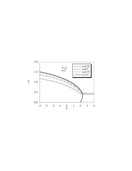
Figure 5: The critical temperature $T_{c}$ as a function of the on-site potential $U$ for $V=-1$, $z=3$ and for $n=0.25$, 0.5, 0.75, 1.

Although below the critical temperature $T_{c}$ the system is thermodynamically unstable, the study of the behavior of relevant parameters below $T_{c}$, unveils the existence of a critical value of the on-site potential separating the two possible realizations of a phase separated region, sketched in Fig 1. In Figs. 6 we plot the double occupancy $D$, the short-range correlation function $\lambda^{(1)}$ and the internal energy $E$ as functions of $U$ at half filling and various temperatures.

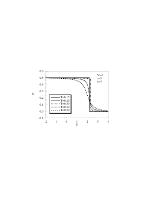
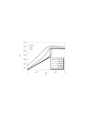
Figure 6: (a) The double occupancy $D$, (b) the short-range correlation function $\lambda^{\left(1\right)}$ and (c) the internal energy $E$ as functions of $U$ for $V=-1$, $z=3$, $n=1$ and for $T=0.15$, 0.2, 0.3, 0.4, 0.5.

One observes that $D$ and $\lambda^{(1)}$ exhibit two plateaus at low temperatures. In the limit $T\to 0$ there is a discontinuity around $U_{c}\approx 2.3V$ (for $z=3$). For $U>U_{c}$, the double occupancy tends to zero as $T\to 0$, whereas $\lambda^{(1)}$ tends to $1/2$. The repulsion between the electrons on the same site and the concomitant nearest neighbor attraction, leads to a scenario where the electrons tend to cluster together singly occupying neighboring sites. As a consequence, at half filling all sites are singly occupied, whereas for $n<1$ one observes two separated clusters of singly and empty sites. When $U<U_{c}$, one observes a dramatic increase (step-like) of the double occupancy and of the short-range correlation function, namely: $D\to 1/2$ and $\lambda^{(1)}\to 1$. As a consequence, half of the sites are doubly occupied, and $\lambda^{(1)}=1$ indicates that the electrons tend to occupy nearest neighbor sites, arranging to form large domains occupied, leaving the rest of the lattice empty. For $U<U_{c}$ one observes also a dramatic decrease of the internal energy $E$, with a discontinuity as $T\rightarrow 0$ around $U\approx U_{c}$. In Fig. 7 we plot the specific heat $C$ as a function of the temperature $T$ at half filling and for several values of the on-site potential $U$. One observes that, for $U\rightarrow U_{c}$, the peak becomes sharper and a divergence is observed at $U=U_{c}$, confirming the emergence of a critical point.

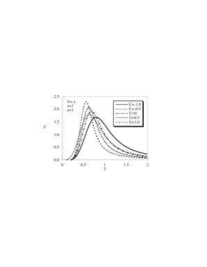
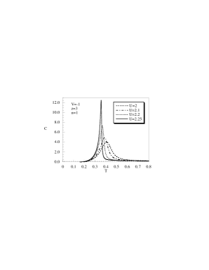
Figure 7: The specific heat $C$ as a function of the temperature $T$ for $V=-1$, $z=3$, $n=1$ and for (a) $U=-1.0$, -0.5, 0, 0.5, $1.0$; (b) $U=2$, 2.1, 2.2, $2.25$.

The same analysis carried out for different values of the particle density, evidences a similar behavior of $D$, $\lambda^{(1)}$ and $E$ as a functions of $U$.

4 Conclusions

In this paper we have obtained the finite temperature phase diagram of a system of fermions with on-site and nearest neighbor interactions localized on the sites of the Bethe lattice. The Hamiltonian describing such a system defines the so-called extended Hubbard model in the atomic limit. By means of the equations of motion method, it is possible to exactly solve the model. For attractive nearest neighbor interaction, by varying the temperature we found a region of negative compressibility, hinting at a transition from a thermodynamically stable to an unstable phase characterized by phase separation. The critical temperature $T_{c}$ at which the transition occurs depends on the filling $n$, on the ratio $U/|V|$ and on $z$. It increases with increasing $z$ and presents a reentrant behavior at half filling for $U/|V|>2$. Even if the region below $T<T_{c}$ is thermodynamically unstable, the study of several thermodynamic quantities allowed us to determine the critical value of the on-site interaction $U_{c}$ separating the formation of clusters of singly and doubly occupied sites. It would be interesting to investigate in detail the structure of the unstable phase as well as to look for a thermodynamically stable phase. This could be done by modifying, for instance, the translational invariance assumption made to obtain the self-consistent equations (16) and (17).

References

- (1) T. Aimi, M. Imada, J. Phys. Soc. Jpn. 76, (2007) 113708.
- (2) A. S. Alexandrov, P. E. Kornilovitch, J. Phys.: Cond. Matt 14, (2002) 5337.
- (3) S. Robaszkiewicz, Acta Phys. Pol. A 45, (1974) 289; K. Rosciszewski, A. M. Oles, J. Phys.: Cond. Matt 15, (2003) 8363; Y. Z. Zhang, T. Minh-Tien, V. Yushankhai, P. Thalmeier, Eur. Phys. J. B 44, (2005) 265.
- (4) J. Solyom, Adv. Phys. 28,(1979) 201.
- (5) B. Fourcade, G. Sproken, Phys. Rev. B 29, (1984) 5089.
- (6) A. Luther, I. Peschel, Phys. Rev. B 9, (1974) 2911; J. Voit, Phys. Rev. B 45, (1992) 4027.
- (7) L. Milas del Bosch, L. M. Falicov, Phys. Rev. B 37 , (1988) 6073; B. Fourcade, G. Sproken, Phys. Rev. B 29, (1984) 5096.
- (8) A. W. Sandvik, L. Balents, D. K. Campbell, Phys. Rev. Lett. 92, (2004) 236401; K. M. Tam, S. W. Tsai, D. K. Campbell, Phys. Rev. Lett. 96, (2006) 036408; S. Glocke, A. Klumper, J. Sirker, Phys. Rev. B 76, (2007) 155121.
- (9) V. J. Emery, Phys. Rev. B 14, (1976) 2989; M. Fowler, Phys. Rev. B 17, (1978) 2989.
- (10) F. Mila, X. Zotos, Europhys. Lett. 24, (1993) 133; K. Penc, F. Mila, Phys. Rev. B 49, (1994) 9670.
- (11) H. Q. Lin, D. K. Campbell, R. T. Clay, Chinese J. Phys. 38, (2000) 1; A. T. Hoang, P. Thalmeier, J. Phys.: Condens. Matt. 14, (2002) 6639; N. H. Tong, S. Q. Shen, R. Bulla, Phys. Rev. B 70, (2004) 085118.
- (12) A. Avella, F. Mancini, Eur. Phys. J. B 41, (2004) 149.
- (13) Y. Tomioka, A. Asamitsu, H. Kuwahara, J. Phys. Soc. Jpn. 66, (1997) 302; T. Kimura, Y. Tokura, J. Q. Li, Y. Matsui, Phys. Rev. B 58, (1998) 11081; T. Chatterji, G. J. McIntyre, W. Caliebe, R. Suryanarayaman, A. Revcolevschi, Phys. Rev. B 61, (2000) 570.
- (14) A. M. Gabovich, A. I. Voitenko, M. Ausloos, Phys. Rep. 367, (2002) 583.
- (15) T. Goto, B. Luthi, Adv. Phys. 52, (2003) 67.
- (16) M. S. Reis, V. S. Amaral, J. P. Araujo, P. B. Tavares, A. M. Gomes, I. S. Oliveira, Phys. Rev. B 71, (2005) 144413.
- (17) M. Imada, A. Fujimori, Y. Tokura, Rev. Mod. Phys. 70, (1998) 1039.
- (18) H. Seo, C. Hotta, H. Fukuyama, Chem. Rev. 104, (2004) 5005.
- (19) E. Dagotto, Nanoscale Phase Separation and Colossal Magnetoresistance (Berlin, Springer-Verlag, 2002).
- (20) G. Pawłowski, T. Kazmierczak, Sol. Stat. Comm. 145, (2008) 109.
- (21) P. G. J. van Dongen, Phys. Rev. Lett. 74, (1995) 182; R. Pietig, R. Bulla, S. Blawid, Phys. Rev. Lett. 82, (1999) 4046.
- (22) T. Misawa, Y. Yamaji, M. Imada, J. Phys. Soc. Jpn.75, (2006) 064705.
- (23) T. Itou, K. Kanoda, K. Murata, T. Matsumoto, K. Hirai, T. Takahashi, Phys. Rev. Lett. 93, (2004) 216408.
- (24) R. A. Bari, Phys. Rev. B 3, (1971) 2662.
- (25) B. Lorenz, Phys. Stat. Sol. (b) 106, (1981) K17.
- (26) G. Beni, P. Pincus, Phys. Rev. B 9, (1974) 2963.
- (27) R. S. Tu, T. A. Kaplan, Phys. Stat. Sol. (b) 63, (1974) 659.
- (28) T. M. Rice, L. Sneddon, Phys. Rev. Lett. 47, (1981) 689.
- (29) R. Micnas, S. Robaszkiewicz, K. A. Chao, Phys. Rev. B 29, (1984) 2784.
- (30) R. J. Bursill, C. J. Thompson, J. Phys. A 26, (1993) 4497.
- (31) M. Bartkowiak, J. A. Henderson, J. Oitmaa, P. E. de Brito, Phys. Rev. B 51, (1995) 14077; E. Halvorsen, M. Bartkowiak, Phys. Rev. B 63, (2000) 014403.
- (32) J. Jedrzejewski, Physica A 205, (1994) 702; C. Borgs, J. Jedrzejewski, R. Kotecky, J. Phys. A 29, (1996) 733.
- (33) F. Mancini, Eur. Phys. J. B 45, (2005) 497; Eur. Phys. J. B 47, (2005) 527.
- (34) F. Mancini, F. P. Mancini, Phys. Rev. E 77, (2008) 061120.
- (35) G. Pawłowski, Eur. Phys. J. B 53, (2006) 471.
- (36) F. Mancini, F. P. Mancini, A. Naddeo, J. Opt. Adv. Mat. 10, (2008) 1688.
- (37) D. Volko, K. F. Quader, arXiv:0710.0023.
- (38) D. Jaksch, Nature 442, (2006) 147.
- (39) F. Mancini, Europhys. Lett. 70, (2005) 485.
- (40) F. Mancini, A. Naddeo, Phys. Rev. E 74, (2006) 061108.
- (41) F. Mancini, A. Avella, Eur. Phys. J. B 36, (2003) 37; Adv. Phys. 53, (2004) 537.