Super universality of the quantum Hall effect and the “large $N$ picture” of the $\vartheta$ angle

Abstract

It is shown that the “massless chiral edge excitations” are an integral and universal aspect of the low energy dynamics of the $\vartheta$ vacuum that has historically gone unnoticed. Within the $SU(M+N)/S(U(M)\times U(N))$ non-linear sigma model we introduce an effective theory of “edge excitations” that fundamentally explains the quantum Hall effect. In sharp contrast to the common beliefs in the field our results indicate that this macroscopic quantization phenomenon is, in fact, a super universal strong coupling feature of the $\vartheta$ angle with the replica limit $M=N=0$ only playing a role of secondary importance. To demonstrate super universality we revisit the large $N$ expansion of the $CP^{N-1}$ model. We obtain, for the first time, explicit scaling results for the quantum Hall effect including quantum criticality of the quantum Hall plateau transition. Consequently a scaling diagram is obtained describing the cross-over between the weak coupling “instanton phase” and the strong coupling “quantum Hall phase” of the large $N$ theory. Our results are in accordance with the “instanton picture” of the $\vartheta$ angle but fundamentally invalidate all the ideas, expectations and conjectures that are based on the historical “large $N$ picture.”

1 Introduction

1.1 Super universality

In a series of investigations on the grassmannian $SU(M+N)/S(U(M)\times U(N))$ non-linear sigma model in two dimensions it was shown that the $\vartheta$ vacuum generally displays massless excitations that propagate along the confining “edge” of the system.[1, 2, 3, 4, 5] This new aspect of the sigma model has come in many ways as a welcome surprise. In applications to quantum spin liquids, [6] for example, the edge excitations describe the dynamics of the “dangling” quantum spins located at the “edges” of the spin chain. [4, 5] In the context of quantum Hall liquids, [7] on the other hand, these excitations are identically the same as those described by the theory of “chiral edge bosons.” [2, 3] Quite similar to the semiclassical ideas that are popularly used for quantum Hall systems [8] one may formulate a percolating network of “edge” excitations while ignoring all the other excitations in the problem. One can then show that in the limit of large distances the network model is identically the same as the original non linear sigma model. [2, 3] The “edge” of the $\vartheta$ vacuum is therefore the key for resolving longstanding issues such as the cross-over between percolation and localization which is known to complicate the experiment on scaling conducted on realistic quantum Hall samples. [9]

Massless chiral edge excitations furthermore lay the bridge between the $\vartheta$ angle concept on the one hand, and the phenomenological approaches to the fractional quantum Hall effect based on Chern-Simons gauge theory on the other.[10] This has led, amongst many other things, to a complete Luttinger liquid theory of edge excitations that includes the effects of disorder, the Coulomb interaction as well as the coupling of the theory to external potentials. [3]

These specific examples clearly indicate that the topological concept of a $\vartheta$ angle is much richer and more profound than previously thought. Notice that the physics of the “edge” would already be a useful advance even if its relevance was limited to the two dimensional electron gas or quantum spin chains alone. This kind of knowledge becomes only more interesting, however, if it turns out that the quantum Hall effect has, in fact, a much more general significance that eventually could shed some new light on the strong coupling problems in QCD where the topological concept of a $\vartheta$ vacuum arose first. [11] Within the grassmannian sigma model one finds, for example, that the $SU(M+N)$ symmetry is spontaneously broken at the “edge” of the system whereas the critical correlations along the “edge” are identically the same for all values of $M$ and $N$. [2] These unexpected features have motivated several studies where the idea of super universality has emerged. [4, 5, 12, 13, 14] The essence of this idea is that the $\vartheta$ vacuum displays all the basic aspects of the quantum Hall effect for all non-negative values of $M$ and $N$. These include not only the massless chiral edge excitations but also the existence of robust topological quantum numbers that explain the precision and stability of the quantum Hall plateaus, as well as the existence of gapless bulk excitations at $\vartheta=\pi$ that describe a quantum phase transition between adjacent plateaus.

The statement of super universality is important because it explains in a natural manner why completely different theories of the $\vartheta$ angle display the same physical phenomena. It encompasses the concept of ordinary universality in critical phenomena phenomenology which is a statement made on critical exponent values alone. Quantum criticality at $\vartheta=\pi$ may in principle be different depending on the specific application of the $\vartheta$ angle that one is interested in. This aspect of the problem is in many ways the same as quantum criticality in $2+\epsilon$ dimensions where each value of $M$ and $N$ is known to describe a different universality class.[15]

Several interesting examples of super universality have already emerged in recent years. We mention, in particular, the Finkelstein approach to localization and interaction effects [13] which explains why the infinitely ranged Coulomb interaction does not affect the basic phenomena of scaling as predicted by the free electron gas [17] and observed in the experiment.[18] The Finkelstein approach, however, fundamentally alters our understanding of the quantum critical behavior of the electron gas. This behavior actually belongs to a novel non-Fermi liquid universality class with a different meaning for the critical exponents [13, 16] and characterized by a previously unrecognized interaction symmetry termed $\mathcal{F}$ invariance. [1] A second example is the Ambegaokar-Eckern-Schön model of the Coulomb blockade.[19] This theory of the $\vartheta$ angle is perhaps the simplest of all since it involves a single abelian field variable in one dimension. Yet it shows all the richly complex physics of quantum Hall liquids and quantum spin liquids.[14]

1.2 Large $N$ expansion

In this investigation we embark on a third example of super universality, the large $N$ expansion of the $CP^{N-1}$ model which is obtained from the grassmannian theory by putting $M,N$ equal to $1,N-1$. This specific case is interesting because it is one of view places in the theory where the $\vartheta$ vacuum is accessible from the strong coupling side. Even though the matter has been studied in detail and elaborated upon a long time ago, [20, 21, 22] it turns out that the physics of the “edge” is a source of unforseen and troublesome complexity that has direct consequences for our understanding of the theory as a whole. We will show that the large $N$ steepest descend methodology, which is standardly performed for an infinite system, misses all the subtle aforementioned features of the confining “edge” of the $\vartheta$ vacuum. The historical papers on the subject mishandle the “massless chiral edge excitations” in the problem and, hence, the most interesting aspect of the $\vartheta$ angle, the quantum Hall effect, remained concealed. The large $N$ analysis that follows is in many ways a completely novel theory. It not only resolves many longstanding controversies on topological issues in both quantum field theory [23] and condensed matter theory [24, 25, 26, 27, 28] but also demonstrates in an unequivocal manner that the $\vartheta$ angle is, in fact, the fundamental theory of the quantum Hall effect.[7, 29]

To obtain the correct low energy dynamics of the $\vartheta$ angle, notably the quantum Hall effect, one must handle the large $N$ steepest descend methodology very differently from what has been done before. Since the massless “edge” excitations are distinctly different from those of the “bulk” of the system they should be disentwined and studied separately. This can in general been done because of their simple topological properties. [2] More specifically, the “edge” excitations generally have a fractional topological charge whereas the “bulk” excitations always carry a strictly integral topological charge. Separating the “edge” from the “bulk” is therefore synonymous for separating the fractional topological sectors of the theory from the integral sectors.

The crux of this investigation is the introduction of an effective theory of “edge” excitations that is obtained by formally eliminating the “bulk” degrees of freedom. This effective theory expresses the low energy dynamics of the $\vartheta$ vacuum in terms of two “physical observables” only. These two quantities have previously been identified as the longitudinal conductance and Hall conductance respectively in the context of the disordered electron gas. [7, 29] We present a comprehensive study of these physical quantities on both the weak and the strong coupling side of the problem. The picture that emerges is precisely in accordance with the renormalization group ideas on the quantum Hall effect that have originally been proposed on the basis of the semiclassical instanton methodology alone.[17, 30, 31] Unlike the previous situation, however, we now have - for the first time - an explicit demonstration of the robust quantization of the Hall conductance together with explicit scaling results for the quantum Hall plateau transition.

1.3 Outline of this work

In order to properly account for the new physics associated with the “edge,” we will present our findings for the large $N$ expansion in a step by step manner. We start out, in Section 2, with a brief summary of the microscopic origins of the $\vartheta$ angle followed by a brief introduction to subject of massless chiral edge excitations. In Section 3 we embark on the general question of how to disentwine the massless edge excitations from the bulk degrees of freedom. The effective theory of massless “edge” excitations is introduced in Section 3.4. This effective theory leads directly to a generalized Thouless criterion for the quantum Hall effect which relates the generation of a mass gap for bulk excitations to the insensitivity of the system to changes in the boundary conditions. The argument is based on very general principles only and therefore sets the stage for the concept of super universality.

After these preliminaries we specialize to the large $N$ expansion of the $CP^{N-1}$ model. In Section 4 we elaborate on the results recently obtained from the instanton calculational technique [12] which is the starting point of the remainder of this paper. In Section 5 we review the standard large $N$ saddle point methodology and show that it conflicts with super universality. We then point out, in Section 6, that the idea of the massless “edge” excitations fundamentally alters the structure of the steepest descend methodology with direct consequences for the “bulk” of the system. We evaluate the effective theory of massless chiral edge excitations and obtain explicit scaling results for the quantum Hall effect and the quantum Hall plateau transitions that were previously invisible. In Section 6.3 we elaborate on the physics of the plateau transitions and show that they are a prototypical example of broad “conductance” distributions in the quantum theory of metals. In Section 6.4 we show how the effective theory of the “edge” can be used as a important check on the Levine-Libby-Pruisken argument for de-localized or gapless “bulk” excitations at $\vartheta=\pi$. [7] These excitations do exist in the large $N$ theory even though the transition is a first order one.

In Section 7 we embark on the cross-over between the weak and strong coupling phases of the large $N$ theory. We first show that the results of the large $N$ steepest descend methodology can in general be decomposed in a discrete set of topological sectors in complete accordance with the semiclassical theory based on instantons. [11, 32, 33] We then show that the “dilute instanton gas” expressions for the free energy and the renormalization group $\beta$ functions retain their general form in the entire range from weak coupling all the way down to the strong coupling phase of the large $N$ theory. The main results of this paper are summarized by the renormalization group flow diagram of the “conductances” plotted in Fig. 4. This paper ends (Section 8) with a summary of the results and a conclusion.

2 The $\vartheta$ angle and physics of the “edge”

The non-linear sigma model representation of Anderson localization in two dimensions and in a perpendicular magnetic field is discussed in detail in Ref. [29]. It involves the grassmannian field variable $Q$ with $Q^{2}={\bf 1}_{M+N}$ that can be written in a standard fashion as follows

$$Q=T^{-1}\Lambda T.$$ (1)

Here, $T\in SU(M+N)$ and $\Lambda$ denotes a diagonal matrix with $M$ elements $+1$ and $N$ elements $-1$

$$\Lambda=\begin{pmatrix}\mathbf{1}_{M}&0\\ 0&-\mathbf{1}_{N}\end{pmatrix}.$$ (2)

The action of the electron gas reads

$$S[Q] = S_{\sigma}[Q]+\pi\omega\rho\int d^{2}x\,\operatorname{tr}\Lambda Q$$ (3)

$$S_{\sigma}[Q] = -\frac{1}{8}g_{0}\int d^{2}x\,\operatorname{tr}\partial_{\mu}Q\partial_{\mu}Q+\frac{1}{8}\sigma^{0}_{H}\int d^{2}x\,\operatorname{tr}\varepsilon_{\mu\nu}Q\partial_{\mu}Q\partial_{\nu}Q.$$ (4)

The dimensionless quantities $g_{0}$ and $\sigma_{H}^{0}$ are the mean field parameters for longitudinal conductance and Hall conductance respectively in units of $e^{2}/h$. The quantity $\rho$ denotes the density of electronic levels and $\omega$ the external frequency.

The success of the non-linear sigma model representation of Anderson localization ultimately relies on our ability to evaluate the Kubo expressions for the macroscopic conductances. These quantities are usually defined for a fixed frequency $\omega$ and an arbitrarily large sample size. They are most elegantly represented in terms of a background matrix field $t(x)\in SU(M+N)$ that varies slowly in space. The master formulae for the background field action reads as follows

$$\exp\{-\mathcal{F}+S^{\prime}_{\sigma}[t]\} = \int\mathcal{D}[Q]\exp\left\{S_{\sigma}[t^{-1}Qt]+\pi\omega\rho\int d^{2}x\,\operatorname{tr}\Lambda Q\right\}.$$ (5)

Here, $\mathcal{F}$ denotes the free energy and the action $S^{\prime}[t]$ is the shift away from the equilibrium distribution as a result of the background field insertion $t(x)$. Provided $t(x)$ satisfies the classical equations of motion this action takes on the form of the sigma model itself

$$S^{\prime}_{\sigma}[t] = -\frac{1}{8}g^{\prime}(\omega)\int d^{2}x\,\operatorname{tr}\partial_{\mu}v\partial_{\mu}v+\frac{1}{8}\sigma^{\prime}_{H}(\omega)\int d^{2}x\,\operatorname{tr}\varepsilon_{\mu\nu}v\partial_{\mu}v\partial_{\nu}v$$ (6)

with ${v}=t^{-1}\Lambda t$. This result is the only possible local action with at most two derivatives that is compatible with the symmetries of the problem. One therefore expects that Eq. (6) has a quite general significance that is independent of $M$ and $N$. In particular, the quantities of physical interest are $g^{\prime}(\omega)$ and $\sigma^{\prime}_{H}(\omega)$ in Eq. (6) which in the replica limit $M,N\rightarrow 0$ precisely correspond to the Kubo expressions for linear response averaged over the impurity ensemble.

2.1 Spontaneous symmetry breaking at the “edge”

The massless excitations along the “edge” of the $\vartheta$ vacuum were recognized first in Refs [2, 3]. To understand this important aspect of the problem we consider the simplest possible scenario of an electron gas in a strong perpendicular magnetic field such that the disordered Landau bands are well separated. By taking the Fermi level $E_{F}$ inside a Landau gap then both quantities $g_{0}$ and $\rho$ in Eq. (4) become zero as it should be. The mean field Hall conductance, however, is strictly integer valued $\sigma_{H}^{0}=k$ with $k$ denoting the number of completely filled Landau levels. [29] The action of Eq. (4) now arises solely from the one dimensional “edge” of the system and we can write

$$S[Q]\rightarrow S_{gap}[Q] = \frac{k}{2}\oint dx\,\operatorname{tr}T\partial_{x}T^{-1}\Lambda+\pi\omega\rho_{\textrm{edge}}\oint dx\,\operatorname{tr}\Lambda Q.$$ (7)

Here, we have made use of the fact that the topological charge can be written as an integral along the edge $\oint$ according to

$$\mathcal{C}[Q]=\frac{1}{16\pi i}\int d^{2}x\operatorname{tr}\epsilon_{\mu\nu}Q\partial_{\mu}Q\partial_{\nu}Q = \frac{1}{4\pi i}\oint dx\,\operatorname{tr}T\partial_{x}T^{-1}\Lambda.$$ (8)

The extra term with $\rho_{\textrm{edge}}$ in Eq. (7) indicates that although there are no electronic levels near $E_{F}$ in the bulk of the system there is nevertheless a finite density of “edge states” that carry the Hall current. Surprisingly, this one dimensional theory is critical and exactly solvable.[2] It can be shown that Eq. (7) is completely equivalent to the theory of chiral edge bosons with the drift velocity $v_{d}$ of the chiral edge electrons given by $v_{d}={k}/{2\pi\rho_{\textrm{edge}}}$. [3] Some important correlations are as follows [2]

$$\langle Q\rangle_{\textrm{edge}}=\Lambda$$ (9)

indicating that the $SU(M+N)$ symmetry is spontaneously broken at the edge of the $\vartheta$ vacuum. Furthermore

$$\langle Q^{+-}_{\alpha\beta}(x)Q^{-+}_{\beta\alpha}(x^{\prime})\rangle_{\textrm{edge}}=4\vartheta(x^{\prime}-x)e^{-\omega(x^{\prime}-x)/v_{d}}$$ (10)

where $Q^{+-}_{\alpha\beta}$ and $Q^{-+}_{\alpha\beta}$ denote the $M\times N$ components in the off-diagonal blocks and $\vartheta(x)$ is the Heaviside step function. The remarkable and surprising feature of these critical edge correlations is that they are completely independent of $M$ and $N$. Moreover, if we interpret the edge coordinate $x$ as the imaginary time $\tau$ then one recognizes Eq. (7) as the bosonic path integral of an $SU(M+N)$ spin with quantum number $s=k/2$ in a magnetic field $B=\rho_{edge}\omega$. [4]

Next, to compute the conductances we go back to our master formulae of Eqs (5) and (6) and write

$$\exp\{-\mathcal{F}+S^{\prime}_{\sigma}[t]\} = \int\mathcal{D}[Q]\exp\left\{S_{\sigma}[t^{-1}Qt]+\pi\omega\rho\oint dx\,\operatorname{tr}\Lambda Q\right\}$$ (11)

$$= \int\mathcal{D}[Q]\exp\left\{S_{gap}[Q]+\frac{k}{2}\oint dx\,\operatorname{tr}t\partial_{x}t^{-1}Q\right\}.$$

We immediately obtain

$$S^{\prime}_{\sigma}[t]=\frac{k}{2}\oint dx\,\operatorname{tr}t\partial_{x}t^{-1}\langle Q\rangle_{edge}=2\pi ik\mathcal{C}[v]$$ (12)

where we have used Eqs (8) and (9). The conductance parameters are therefore independent of $M$ and $N$ and given by

$$g^{\prime}(\omega)=0~{}~{},~{}~{}~{}\sigma_{H}^{\prime}(\omega)=k.$$ (13)

We see that the quantum Hall effect reveals itself through spontaneous symmetry breaking at the “edge” of the $\vartheta$ vacuum. This unexpected feature of the sigma model in two dimensions has historically been overlooked. From now onward we recognize the action of Eq. (7) as the critical fixed point action of the quantum Hall state.

3 Disentangling the bulk and the edge

3.1 The matrix field variable $Q$

To disentwine the massless “edge” excitations from the “bulk” excitations we write

$$Q=\varphi^{-1}Q_{0}\varphi$$ (14)

where $Q_{0}=T_{0}^{-1}\Lambda T_{0}$ has a fixed value $Q_{0}=\Lambda$ at the edge. The matrix $\varphi\in SU(M+N)$ generally stands for the “fluctuations” about these special boundary conditions. These distinctly different components of $Q$ are termed the “bulk” component and “edge” component respectively. They are topologically classified according to

$$\mathcal{C}[Q]=\mathcal{C}[Q_{0}]+\mathcal{C}[q]~{}~{},~{}~{}~{}q=\varphi^{-1}\Lambda\varphi$$ (15)

where $\mathcal{C}[Q_{0}]$ is by construction an integer and $-\frac{1}{2}<\mathcal{C}[q]\leq\frac{1}{2}$ stands for the fractional part of $\mathcal{C}[Q]$. Notice that for the special case of integer filling fractions $\nu$ the action (Eq. 7) solely depends on the “edge” component $\varphi$ of $Q$

$$S_{gap}[Q]=S_{gap}[\varphi^{-1}Q_{0}\varphi] = \frac{k}{2}\oint dx\,\operatorname{tr}\left[\varphi\partial_{x}\varphi^{-1}+\frac{\omega}{v_{d}}q\right]\Lambda+2\pi ik\mathcal{C}[Q_{0}].$$ (16)

The “bulk” component $Q_{0}$ gives rise to a trivial phase factor $2\pi ik\mathcal{C}[Q_{0}]$ and can be ignored.

3.2 The $\vartheta$ parameter or $\sigma_{H}^{0}$

Next, to address the general theory of Eq. (4) it is convenient split the mean field parameter $\sigma_{H}^{0}=\nu$ into an integral piece $k(\nu)$ and a fractional piece $-\pi<\theta(\nu)\leqq\pi$ according to (see Figs 1 and 2)

$$\sigma_{H}^{0}=\nu=k(\nu)+\frac{\theta(\nu)}{2\pi}.$$ (17)

Microscopically, i.e. for the electron gas in strong magnetic fields, the quantities $k(\nu)$ and $\theta(\nu)$ appear as distinctly different contributions from the “edge” and the “bulk” respectively. [34] The mean field parameters $g_{0}=g_{0}(\theta(\nu))$ and $\rho=\rho(\theta(\nu))$ are typical “bulk” quantities that for a given Landau band depend on $\theta(\nu)$ only. They are symmetric under $\theta(\nu)\Leftrightarrow-\theta(\nu)$ which is termed “particle-hole” symmetry.

The split in Eq. (17) can easily be understood by considering a system with a “clean” confining edge that is spatially separated from the homogenously distributed disorder in the interior of the system. This kind of thought experiment has frequently been used in Refs [2, 3] and here it shows that the integral piece $k(\nu)$ typically arises from the “edge” states in the problem that are unaffected by the disorder whereas $\theta(\nu)$, like $g_{0}(\theta(\nu))$ and $\rho(\theta(\nu))$, is entirely determined by the disorder in the “bulk” of the system.

3.3 Actions for the “bulk” and the “edge”

Using these definitions we next split Eqs (3) and (4) into a “bulk” part $S_{bulk}$ and an “edge” part $S_{edge}$ as follows

$$S[Q] = S_{bulk}[Q]+S_{edge}[q]$$ (18)

$$S_{bulk}[Q] = \tilde{S}_{\sigma}[Q]+\pi\omega\rho\int d^{2}x\,\operatorname{tr}Q\Lambda$$ (19)

$$S_{edge}[q] = 2\pi ik(\nu)\mathcal{C}[q]+\pi\omega\rho_{edge}\oint dx\,\operatorname{tr}q\Lambda.$$ (20)

Here, $\tilde{S}_{\sigma}[Q]$ denotes the sigma model for the “bulk” of the system

$$\tilde{S}_{\sigma}[Q] = -\frac{g_{0}}{8}\int d^{2}x\,\operatorname{tr}\partial_{\mu}Q\partial_{\mu}Q+i\theta(\nu)\mathcal{C}[Q].~{}~{}~{}$$ (21)

By separating the integrals over the “bulk” modes $Q_{0}$ and “edge” components $q$ or $\varphi$ we can write

$$Z = \int\mathcal{D}[q]~{}e^{S_{edge}[q]}~{}\int_{\partial V}\mathcal{D}[Q_{0}]~{}e^{S_{bulk}[\varphi^{-1}Q_{0}~{}\varphi]}.$$ (22)

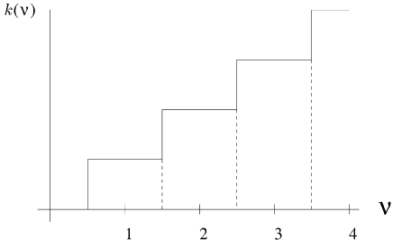
Figure 1: The edge part of $\sigma_{H}^{0}$ with varying $\nu$, see text.

Figure 2: The bulk part of $\sigma_{H}^{0}$ with varying $\nu$, see text.

Here, the subscript $\partial V$ reminds us of the fact that the functional integral over $Q_{0}$ has to be performed with fixed boundary conditions $Q_{0}=\Lambda$. Notice that for integer filling fractions $\nu$ the action $S_{bulk}$ is zero and Eq. (22) stands for the critical theory of the “edge” as it should be. On the other hand, in the absence of the “edge” component $\varphi$ or $q$ we obtain a theory of pure “bulk” excitations $S_{bulk}[Q_{0}]$ with a strictly quantized topological charge $\mathcal{C}[Q_{0}]$. This theory is precisely in accordance with the semiclassical “instanton picture” of the $\vartheta$ angle.

As a final remark, it should be mentioned that the results of this Section have a quite general significance that is independent of condensed matter applications. For example, the split written in Eq. (18) can always be made even though the decomposition of Eq. (17) may not always be physically obvious. The main advantage of the electron gas, therefore, is that the distinction between the “bulk” and “edge” naturally emerges from the microscopic origins of the $\vartheta$ angle.

3.4 Finite size scaling

We are now in a position to introduce finite size scaling ideas for the macroscopic conductances. For this purpose we take the limit $\omega=0$ in the action for the “bulk” $S_{bulk}$ and let the infrared be defined by the sample size $\lambda^{\prime}$. Eq. (22) can now be written in terms of an effective theory for the “edge” according to

$$Z = e^{-\mathcal{F}_{b}}\int\mathcal{D}[q]~{}e^{S_{edge}[q]+\tilde{S}^{\prime}_{\sigma}[q]}$$ (23)

where

$$e^{-\mathcal{F}_{b}+\tilde{S}^{\prime}_{\sigma}[q]} = \int_{\partial V}\mathcal{D}[Q_{0}]e^{\tilde{S}_{\sigma}[\varphi^{-1}Q_{0}~{}\varphi]}.$$ (24)

Here, $\mathcal{F}_{b}=\mathcal{F}_{b}(\theta(\nu))$ denotes the “bulk” free energy. Notice that the effective action $\tilde{S}^{\prime}_{\sigma}[q]$ is, in effect, a measure for the sensitivity of the “bulk” of the system to infinitesimal changes in the boundary conditions. Emerging from Eqs (23) and (24) is therefore the well known “scaling picture” of Anderson localization where one divides the macroscopic system into an array of much smaller “blocks” of size $\lambda\ll\lambda^{\prime}$. Provided the $\varphi$ field obeys the classical equations of motion one can generally express the effective action $\tilde{S}^{\prime}_{\sigma}[q]$ as follows

$$\tilde{S}^{\prime}_{\sigma}[q] = -\frac{1}{8}g^{\prime}(\lambda)\int d^{2}x\,\operatorname{tr}\partial_{\mu}q\partial_{\mu}q+i\theta^{\prime}(\lambda)\mathcal{C}[q]~{}~{}~{}$$ (25)

where $g^{\prime}(\lambda)$ and $\theta^{\prime}(\lambda)$ are the “response” parameters associated with a single block. They are explicitly given as correlations of the Noether current $J_{\mu}=Q_{0}\partial_{\mu}Q_{0}$ according to [31, 29]

$$g^{\prime}(\lambda) = g_{0}+\frac{(g_{0})^{2}}{8MN\lambda^{2}}\int_{x,x^{\prime}}\langle\operatorname{tr}J_{\mu}(x)J_{\mu}(x^{\prime})\rangle$$ (26)

$$\theta^{\prime}(\lambda) = \theta(\nu)+\frac{(g_{0})^{2}}{8MN\lambda^{2}}\int_{x,x^{\prime}}\langle\operatorname{tr}\varepsilon_{\mu\nu}J_{\mu}(x)J_{\nu}(x^{\prime})\Lambda\rangle$$ (27)

where the expectations $\langle\dots\rangle$ are with respect to $\tilde{S}_{\sigma}[Q_{0}]$ which is defined for a block of size $\lambda$. Here, $g^{\prime}(\lambda)$ stands for the parallel conductance and

$$\sigma^{\prime}_{H}(\lambda) = k(\nu)+\frac{\theta^{\prime}(\lambda)}{2\pi}~{}~{}~{}$$ (28)

denotes the Hall conductance. By considering a sequence of scale sizes $\lambda$, $2\lambda$, $4\lambda$ etc. then the results of Eqs (26) - (28) essentially tell us how single blocks are being joined together to form the transport parameters of bigger blocks. This scaling scenario immediately suggests a generalized Thouless criterion for Anderson localization in the presence of a magnetic field. More specifically, since exponentially localized electronic levels are insensitive to changes in the boundary conditions one expects that the response parameters $g^{\prime}(\lambda)$ and $\theta^{\prime}(\lambda)$ render exponentially small

$$g^{\prime}(\lambda),~{}\theta^{\prime}(\lambda)\propto~{}\exp\{-\lambda/\xi\}$$ (29)

with $\xi$ denoting the localization length, provided $\lambda$ is taken large enough. Under these circumstances Eqs (23) - (24) scale toward the critical “edge” theory of the quantum Hall state, Eq.(16), with $\sigma_{H}^{\prime}=k(\nu)+\mathcal{O}(e^{-\lambda/\xi})$ now standing for the robustly quantized Hall conductance, see Fig. 1.

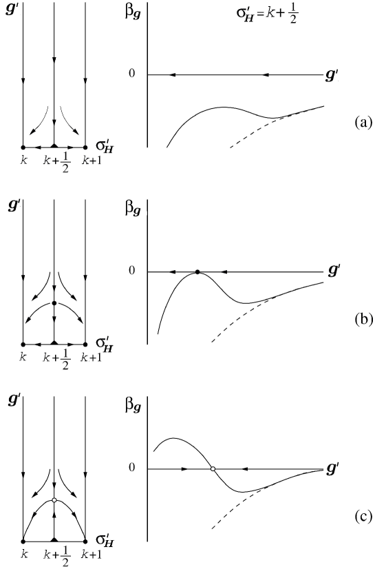
Figure 3: The renormalization group flow diagram in the $g^{\prime}$ - $\sigma^{\prime}_{H}$ “conductance” plane, along with the $\beta_{g}=dg^{\prime}/d\ln\lambda$ function along the line $\sigma_{H}^{\prime}=k+\frac{1}{2}$, for different values of $M$ and $N$. The results show how instanton effects alter the perturbative $\beta_{g}$ functions depicted by the dashed lines. (a) Typical behavior for large values of $M$, $N$. (b) Intermediate behavior that is likely displayed by the theory with $M=N=1$ or the $O(3)$ non-linear $\sigma$ model. (c) Typical behavior for $0\leqq M,N<1$, see text.

Since nothing of the argument seems to crucially depend on the number of field components $M$ and $N$, we expect that this scaling picture has a quite general significance for the theory for all values $M,N\geq 0$. Indeed, the explicit results for Eqs (26) - (28) obtained from the instanton calculational technique [12] are all in accordance with the Thouless criterion and the super universality concept discussed earlier, see Fig. 3. On the other hand, since the theory is generally inaccessible on the strong coupling side, it is extremely important to have a simple example where the different aspects of the super universality concept can be investigated and explored exactly. For this purpose we specialize from now onward to the large $N$ expansion of the $CP^{N-1}$ model.

4 Weak coupling results at large $N$

From Eqs (23) - (27) we see that the physics of the $\vartheta$ vacuum is in general defined by only three physical quantities, namely the free energy $\mathcal{F}_{b}$ and the response parameters $g^{\prime}$ and $\theta^{\prime}$. These quantities are all defined by the underlying theory of bulk excitations with a strictly quantized topological charge $\mathcal{C}[Q_{0}]$. This means that the $\theta(\nu)$ dependence can be expressed in terms of a series expansion in “discrete topological sectors” $n$ according to

$${(\lambda^{\prime})^{-2}}\mathcal{F}_{b}=\sum_{n=0}^{\infty}\phi_{n}\cos n\theta(\nu)$$ (30)

and

$$g^{\prime}(\lambda^{\prime})=g_{0}+\sum_{n=0}^{\infty}\rho_{n}\cos n\theta(\nu)$$ (31)

$$\theta^{\prime}(\lambda^{\prime})=\theta(\nu)+\sum_{n=1}^{\infty}\xi_{n}\sin n\theta(\nu).$$ (32)

The $\phi_{n}$ , $\rho_{n}$ and $\xi_{n}$ generally stand for functions of $g_{0}$ and the scale size $\lambda^{\prime}$ alone. As we shall see in the remainder of this paper, it is precisely this feature of the theory that eventually facilitates the contact between the weak and strong coupling phases of the large $N$ expansion. We first briefly recall, in Sections 4.1 and 4.2 below, some of the results obtained in the weak coupling instanton phase.[12]

4.1 Free energy

The large $N$ expansion is usually expressed in terms of a re-scaled parameter $g_{0}$

$$\sigma_{0}=g_{0}/N$$ (33)

such that the perturbative quantum corrections to $\sigma_{0}$ are independent of $N$

$$\sigma(\lambda)=\sigma_{0}-\frac{1}{2\pi}\ln\mu\lambda=-\frac{1}{2\pi}\ln\lambda M_{0}.$$ (34)

Here, $M_{0}$ denotes the dynamically generated mass of the large $N$ expansion

$$M_{0}=\mu e^{-2\pi\sigma_{0}}$$ (35)

Within the dilute instanton gas approach one usually deals with only the $n=1$ term in Eq. (30). Using $\sigma$ as a shorthand for $\sigma(\lambda)$ we cast the standard result for large values of $N$ in the following general form

$${(\lambda^{\prime})^{-1}}\mathcal{F}_{b}=-\int\frac{d\lambda}{\lambda^{3}}w(\sigma)W^{N}(\sigma)\cos\theta(\nu)$$ (36)

where $(\lambda^{\prime})^{2}$ denotes the area of the system and the functions $W(\sigma)$ and $w(\sigma)$ are given by

$$W(\sigma)=\exp\left\{-2\pi\sigma+\ln 4\pi\sigma-\gamma-\frac{1}{2}\right\}~{},~{}~{}w(\sigma)=\left({2N}/{\pi}\right)^{3/2}/e$$ (37)

with $\gamma\approx 0.577$ the Euler constant. The unspecified integral over the scale size $\lambda$ in Eq. (36) diverges in the infrared. This notorious drawback dramatically complicates the meaning of the semiclassical methodology. [11, 32] Within the historical large $N$ analysis, for example, it was first assumed that instantons do not contribute. [21] Following the seminal critique by Jevicki [33] this conjecture was later abandoned. [22] The different approaches to the $\vartheta$ vacuum have nevertheless led to an “arena of bloody controversies ” [23] that has not been resolved even to date.

In what follows we shall argue that the results of Eq. (37) can only be trusted in the range $\lambda M_{0}\ll 1$ where one normally expects the perturbative quantum theory to be valid. As one approaches the strong coupling phase $\lambda M_{0}\gtrsim 1$ the integrant of Eq. (36) presumably gets complicated by additional contributions from pairs of instantons and anti-instanton that are difficult incorporate semiclassically. In Section 7 we show how the large $N$ steepest descend methodology can be used to shed new light on the matter. We find, in particular, that the general form of Eq. (36) is retained except that the functions $W(\sigma)$, $w(\sigma)$ and $\sigma(\lambda)$ have a different meaning when $\lambda M_{0}\gtrsim 1$. These extended instanton results are a special case of the more general statement which says that the coefficients $\phi_{n}$ in Eq. (30) are all finite as $\lambda^{\prime}$ goes to infinity.

Even though the new insights into the traditional infrared problems of instantons are important, free energy considerations alone do not teach us much about the singularity structure of the theory as $\theta(\nu)$ approaches $\pm\pi$. The lowest order terms in the series of Eq. (30) generally tell us something about the regular part of the free energy which is of secondary interest.

4.2 Observable theory

To study the low energy dynamics of the $\vartheta$ vacuum, in particular the quantum Hall effect, one must develop a quantum theory of the response parameters $g^{\prime}$ and $\theta^{\prime}$ in Eqs (31) and (32) which we term the observable theory. The results can in general be expressed as an integral over scale sizes $\lambda$

$$\sigma^{\prime}(\lambda^{\prime}) = \sigma^{\prime}(\lambda_{0})+\int_{\lambda_{0}}^{\lambda^{\prime}}\frac{d\lambda}{\lambda}\beta_{\sigma}(\sigma^{\prime},\theta^{\prime})$$ (38)

$$\theta^{\prime}(\lambda^{\prime}) = \theta^{\prime}(\lambda_{0})+\int_{\lambda_{0}}^{\lambda^{\prime}}\frac{d\lambda}{\lambda}\beta_{\theta}(\sigma^{\prime},\theta^{\prime})$$ (39)

where $\sigma^{\prime}=g^{\prime}/N$. The $\beta$ functions extracted from the dilute instanton gas are universal and can be written in the form

$$\beta_{\sigma} = f(\sigma^{\prime})-f_{1}(\sigma^{\prime})~{}W^{N}(\sigma^{\prime})\cos\theta^{\prime}$$ (40)

$$\beta_{\theta} = ~{}~{}~{}~{}~{}~{}~{}-g_{1}(\sigma^{\prime})~{}W^{N}(\sigma^{\prime})\sin\theta^{\prime}$$ (41)

where the function $W$ is the same as in Eq. (37) and the $f$, $g$ functions are given by

$$f(\sigma^{\prime}) = -\frac{1}{2\pi\sigma^{\prime}}$$

$$f_{1}(\sigma^{\prime}) = 8e^{-1}N(2\pi N)^{1/2}~{}\sigma^{\prime}$$

$$g_{1}(\sigma^{\prime}) = 8e^{-1}N(2\pi N)^{3/2}~{}(\sigma^{\prime})^{2}.$$ (42)

In anticipation of our findings in Section 7 we can say that the general form of the $\beta$ functions in Eqs (40) and (41), like the free energy of Eq. (36), is retained all the way down to the strong coupling phase provided one gives a proper meaning to the functions $W$, $f$ and $g$. These generalized instanton results are the lowest order terms in an infinite series that reads

$$\beta_{\sigma} = \sum_{n=0}^{\infty}\beta_{\sigma}^{(n)}(\sigma^{\prime})\cos n\theta^{\prime}$$ (43)

$$\beta_{\theta} = \sum_{n=1}^{\infty}\beta_{\theta}^{(n)}(\sigma^{\prime})\sin n\theta^{\prime}.$$ (44)

On the weak coupling side one expects that the convergence of the series is controlled by instanton factors that are typically of the form

$$\beta_{\sigma}^{(n)}(\sigma),~{}\beta_{\theta}^{(n)}(\sigma)\simeq W^{Nn}(\sigma^{\prime}).$$ (45)

On the strong coupling side we find that the $\beta_{\sigma}$ function as a whole goes to zero and the quantities $\beta_{\theta}^{(n)}(\sigma)$ in Eq. (44) all approach a finite constant in the limit $\sigma^{\prime}\rightarrow 0$. In different words, the large $N$ expansion is the much sought after example where the concept of $\vartheta$ renormalization can be explored and investigated in the entire range from weak to strong coupling.

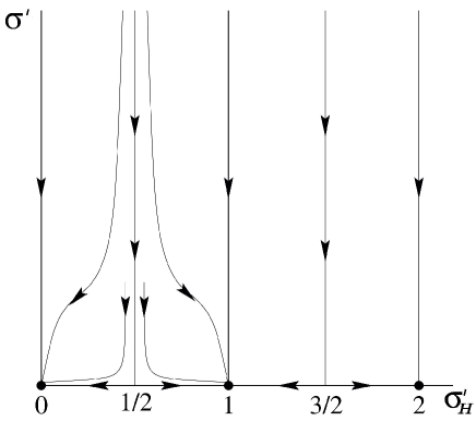
Figure 4: Renormalization group flows in the $\sigma^{\prime}$ - $\sigma_{H}^{\prime}$ “conductance” plane according to the $CP^{N-1}$ theory with large values of $N$, see text.

5 $CP^{N-1}$ model

5.1 Introduction

In this Section we review the various different steps of the large $N$ steepest descend methodology of the $CP^{N-1}$ model. [20, 21, 22] The matrix field variable $Q\in{SU(N)}/{U(N-1)}$ can be expressed in terms of a complex vector field $z_{\alpha}$

$$Q_{\alpha\beta}=2z_{\alpha}^{*}z_{\beta}-\delta_{\alpha\beta}$$ (46)

with ${{z}^{*}_{\alpha}{z}_{\alpha}}=1$. The action is usually taken in $1+1$ space-time dimension and without mass terms

$$S[Q]=\int d^{2}x\,\Bigl{[}-g_{0}\left(\partial_{\mu}z_{\alpha}^{*}\partial_{\mu}z_{\alpha}+z_{\alpha}^{*}\partial_{\mu}z_{\alpha}z_{\beta}^{*}\partial_{\mu}z_{\beta}\right)+\sigma_{H}^{0}~{}\varepsilon_{\mu\nu}\partial_{\mu}z_{\alpha}^{*}\partial_{\nu}z_{\alpha}\Bigr{]}.$$ (47)

Introducing a vector field $A_{\mu}$ one can write

$$S[Q,A_{\mu}]=\int d^{2}x\,\Bigl{[}-g_{0}|D_{\mu}z_{\alpha}|^{2}+i\sigma_{H}^{0}\varepsilon_{\mu\nu}\partial_{\mu}A_{\nu}\Bigr{]}$$ (48)

where $D_{\mu}=\partial_{\mu}+iA_{\mu}$ and the topological charge becomes

$$\mathcal{C}[A_{\mu}]=\frac{1}{2\pi}\int d^{2}x\,\varepsilon_{\mu\nu}\partial_{\mu}A_{\nu}.$$ (49)

Notice that under the shift $A_{\mu}\rightarrow A_{\mu}+iz_{\alpha}^{*}\partial_{\nu}z_{\alpha}$ the $A_{\mu}$ and $z_{\alpha}$ fields decouple and we obtain the original theory of Eq. (47). For the time being we shall ignore the problem of the massless “edge” excitations and assume, following the historical papers, that $A_{\mu}$ is an unconstrained free field. We lift the nonlinearity condition ${z^{*}_{\alpha}z_{\alpha}}=1$ as usual introducing an auxiliary field $\phi(x)$

$$S[Q,A_{\mu},\lambda]=S[Q,A_{\mu}]+ig_{0}\int d^{2}x\,\phi\left(|z_{\alpha}|^{2}-1\right).$$ (50)

The $z_{\alpha}$ vector fields are now free and can be eliminated. This leads to an effective theory in terms of $\phi$ and $A_{\mu}$ fields alone

$$S[A_{\mu},\phi]=-N\left[\operatorname{tr}\ln(-D^{2}+i\phi)-i\sigma_{0}\int d^{2}x~{}\phi\right]+i\sigma_{H}^{0}\int d^{2}x\,\varepsilon_{\mu\nu}\partial_{\mu}A_{\nu}.$$ (51)

We have introduced the quantity $\sigma_{0}=g_{0}/N$ as before. Eq. (51) has an $SU(N)$ invariant stationary point $i\phi(x)=M_{0}^{2}$. Putting $A_{\mu}=0$ we obtain the following expression for the mass $M_{0}$

$$\int\frac{d^{2}k}{(2\pi)^{2}}\frac{1}{k^{2}+M_{0}^{2}}=\sigma_{0}.$$ (52)

Introducing an ultraviolet cutoff $\mu$

$$\sigma_{0}=\frac{1}{2\pi}\ln\frac{\mu}{M_{0}},\qquad M_{0}=\xi^{-1}=\mu e^{-2\pi\sigma_{0}}$$ (53)

we obtain the same results as in Eqs (33) and (35) extracted from ordinary perturbation theory. Next, by neglecting the fluctuations in the $\phi$ field which are of order $N^{-1}$, we expand the theory as a power series in the $A_{\mu}$ field. Assuming Lorentz invariance we obtain the standard result

$$N\operatorname{tr}\ln(-D_{\mu}^{2}+M_{0}^{2})=N\operatorname{tr}\ln(-\partial_{\mu}^{2}+M_{0}^{2})+\frac{N}{48\pi M_{0}^{2}}\int d^{2}x\,F_{\mu\nu}^{2}\hskip 14.22636pt{}$$ (54)

and the effective action reads

$$S[A_{\mu}]=\int d^{2}x\,\Bigl{[}-\frac{N}{48\pi M_{0}^{2}}F_{\mu\nu}^{2}+i\sigma_{H}^{0}~{}\varepsilon_{\mu\nu}\partial_{\mu}A_{\nu}\Bigr{]}.$$ (55)

At this point the historical large $N$ methodology gets complicated. The difficulties are immediately obvious when considering the expression for the free energy

$$\mathcal{F}(\sigma_{H}^{0})=-\ln\int D[A_{\mu}]e^{S[A_{\mu}]}=\frac{12\pi\lambda^{2}M_{0}^{2}}{N}(\sigma_{H}^{0})^{2}$$ (56)

where

$$\lambda^{2}=\beta L$$ (57)

denotes the area in space-time (from now onward we write $\lambda$ for $\lambda^{\prime}$ whenever convenient). Even though Eq. (56) does not display any periodicity in $\sigma_{H}^{0}$, one nevertheless argues on heuristic grounds that Eq. (56) should be periodic. [21, 22] Based on the electrodynamics “picture” by Coleman, [35] for example, one assumes that Eq. (56) is only correct in the interval $-\frac{1}{2}<\sigma_{H}^{0}\leq\frac{1}{2}$. Outside this interval it is energetically favorable for the system to materialize a pair of “charges” that move in opposite directions to the “edges” of the universe such as to maximally shield the background “electric field” $\sigma_{H}^{0}$. Eq. (56) should therefore be expressed in terms of the internally generated “electric field” rather than the bare value $\sigma_{H}^{0}$. We will come back to these ideas in Section 6

5.2 Bulk and edge excitations

Although cleverly designed, Coleman’s ad hoc arguments should not be mistaken for an exact or complete theory of the $\vartheta$ vacuum. To demonstrate that something fundamental is missing we employ the master formulae for the conductances of Section 2. Since the large $N$ methodology is manifestly $SU(N)$ invariant (there is no spontaneous symmetry breaking) the insertion of a background matrix field $t(x)$ is immaterial and we immediately obtain the trivial response

$$g^{\prime}(\omega)=\sigma^{\prime}_{H}(\omega)=0$$ (58)

in the limit $\omega=0$. This result conflicts with the quantum Hall effect, in particular Eq. (13), indicating that the massless chiral “edge” excitations in the problem have been overlooked. These edge excitations have disappeared in Eq. (55) the reason being that incorrect assumptions have been made about the order in which the integrals over the $A_{\mu}$ and $z_{\alpha}$ fields in Eq. (48) must be performed.

Guided by the analysis of Section 3 we next discuss the subtle modifications in the large $N$ methodology that are necessary in order to be able to extract the correct low energy dynamics of the $\vartheta$ vacuum.

1. First, in accordance with Eq. 14 we split the vector field $z_{\alpha}$ in “edge” components $\varphi$ and “bulk” modes $\zeta$ according to

   $$z_{\alpha}=\sum_{\beta=1}^{N}\varphi_{\alpha\beta}\,\zeta_{\beta}.$$ (59)

   Here, the vector field $\zeta_{\alpha}$ is constrained by the boundary condition $\zeta_{\alpha}=e^{i\phi}\delta_{\alpha,1}$ with $\phi$ an arbitrary $U(1)$ gauge.

2. Eq. (59) implies that the topological charge $\mathcal{C}[A_{\mu}]$ in Eqs (48) and (49) must be split into integral and fractional pieces. Specifically, we impose the constraint

   $$\mathcal{C}[A_{\mu}]=n+\mathcal{C}[q]~{},~{}~{}\mathcal{C}[q]=\frac{1}{16\pi i}\oint dx_{\mu}\,\operatorname{tr}\,\epsilon_{\mu\nu}q\partial_{\mu}q\partial_{\nu}q$$ (60)

   where $n$ is an arbitrary integer and $\mathcal{C}[q]$ the fractional piece associated with the “edge” component $\varphi$ or $q=\varphi^{-1}\Lambda\varphi$. Introducing an auxiliary field $\eta$ we incorporate the constraint by substituting

   $$i\sigma_{H}^{0}\int d^{2}x\,\varepsilon_{\mu\nu}\partial_{\mu}A_{\nu} \rightarrow i(\sigma_{H}^{0}-\eta)\int d^{2}x\,\varepsilon_{\mu\nu}\partial_{\mu}A_{\nu}+2\pi i\eta(n+\mathcal{C}[q])$$ (61)

   in Eqs (48) and (49).

3. The steps from Eq. (50) to Eq. (54) are slightly modified since we only integrate over the “bulk” components $\zeta_{\alpha}$ while retaining the “edge” matrix field variable $\varphi$ or $q$. The results are summarized by making the following substitution in Eqs (54) and (55)

   $$\frac{N}{48\pi M_{0}^{2}}\int d^{2}x\,F_{\mu\nu}^{2}\rightarrow\frac{N}{48\pi M_{0}^{2}}\int d^{2}x\,F_{\mu\nu}^{2}+\delta S[q,A_{\mu}].$$ (62)

   Here $\delta S$ stands for all the higher order terms that are irrelevant. The only term of physical interest is the small correction term

   $$\delta S[q,A_{\mu}]=\frac{g^{\prime}(\lambda)}{8}\int d^{2}x\,\operatorname{tr}\partial_{\mu}q\partial_{\mu}q~{},~{}~{}~{}~{}g^{\prime}(\lambda)\approx e^{-\lambda M_{0}}$$ (63)

   that is permitted by the boundary condition imposed on the $\zeta_{\alpha}$ vector field.

By substituting Eqs (61) and (62) in the historical result of Eq. (55) we obtain a more complex theory that besides the $A_{\mu}$ field also depends on the “edge” matrix field variable $q$ as well as the auxiliary field $\eta$ and $n$

$$S[A_{\mu},q,\eta,n] = \int\Bigl{[}-\frac{N}{48\pi M_{0}^{2}}F_{\mu\nu}^{2}+i(\sigma_{H}^{0}-\eta)\varepsilon_{\mu\nu}\partial_{\mu}A_{\nu}\Bigr{]}+$$ (64)

$$~{}~{}~{}~{}~{}~{}~{}~{}~{}~{}~{}~{}~{}~{}~{}~{}~{}~{}~{}~{}~{}~{}~{}~{}~{}~{}~{}~{}~{}~{}~{}+2\pi i\eta(n+\mathcal{C}[q])+\delta S[q,A_{\mu}].$$

At this stage of the analysis several remarks are in order. First of all, it should be mentioned that the piece $\delta S$ in Eq. (64) really describes the correction terms in a systematic expansion in large values of $N$. To see this we re-scale

$$\lambda\rightarrow\lambda\sqrt{N}~{},~{}~{}A_{\mu}\rightarrow A_{\mu}/\sqrt{N}$$ (65)

while keeping the dimensionless quantities $q$, $\eta$ and $n$ unchanged. This removes the factor $N$ from the leading order result in Eq. (64) such that all the $N$ dependence now appears in $\delta S$. For example, the quantity $g^{\prime}(\lambda)$ gets replaced by

$$g^{\prime}(\lambda)\rightarrow g^{\prime}(\sqrt{N}\lambda)\approx e^{-\sqrt{N}\lambda M_{0}}$$ (66)

indicating that physically the large $N$ steepest descend methodology describes a systematic expansion about the strong coupling line $g^{\prime}=0$ in the $g^{\prime}$ - $\sigma_{H}^{\prime}$ conductance plane.

Secondly, from Eq. (63) we infer that the natural scaling parameter $\sigma^{\prime}(\lambda)$ of the large $N$ theory is given by

$$\sigma^{\prime}(\lambda)=g^{\prime}(\lambda)\approx e^{-\lambda M_{0}}\ll 1.$$ (67)

This definition is the strong coupling counter part of the weak coupling statement of Eqs (33) and (34). Since Eq. (67) does not depend on $\theta(\nu)$ we will not distinguish, in what follows, between the observable parameter $\sigma^{\prime}(\lambda)$ and the renormalized quantity $\sigma(\lambda)$ in which the free energy is generally expressed (see, however, Section 7.2.1).

Keeping these remarks in mind we discard, from now onward, the piece $\delta S$ unless explicitly stated otherwise. We proceed by eliminating the $A_{\mu}$ field in Eq. (64) which is now a free field. The effective action in terms of field variables $\eta$, $q$ and $n$ reads

$$S[\eta,q,n]=-\frac{12\pi\lambda^{2}M_{0}^{2}}{N}(\sigma_{H}^{0}-\eta)^{2}+2\pi i\eta(n+\mathcal{C}[q]).$$ (68)

The effective theory of edge excitations is now defined by

$$Z[q]=\sum_{n}\int_{-\infty}^{\infty}d\eta~{}e^{S[\eta,q,n]}.$$ (69)

Notice that the only difference between Eqs (68) and (69) and the original results of Eqs (55) and (56) is the constraint of Eq. (60) that separates the integral topological sectors from the fractional ones. In what follows we shall distinguish between two different strong coupling phases of the theory, termed the quantum Hall phase (Section 6) and the pseudo instanton phase (Section 7) respectively, depending on the value of the dimensionless variable ${12\pi\lambda^{2}M_{0}^{2}}/{N}$.

Figure 5: The bulk free energy $\mathcal{F}_{b}/\lambda^{2}\propto\theta^{2}(\nu)$ with varying $\nu$, see text.

6 Quantum Hall phase ${12\pi\lambda^{2}M_{0}^{2}}/{N}\gg 1$

By making use of the Poisson summation formula

$$\sum_{n}e^{2\pi i\eta n}=\frac{1}{2\pi}\sum_{m}\delta(\eta-m)$$ (70)

we can express Eqs (68) and (69) as sum over integers $m$

$$Z[q]=\sum_{m}\exp\left\{-\frac{12\pi\lambda^{2}M_{0}^{2}}{N}(\sigma_{H}^{0}-m)^{2}+2\pi im\mathcal{C}[q]\right\}.$$ (71)

This sum is rapidly converging in the limit where $\lambda\rightarrow\infty$ while keeping all the other parameters in the problem fixed. Let us next compare the completely different results that are obtained depending on the interpretation of the topological charge of the $A_{\mu}$ vector field.

1. If one assumes, in accordance with the historical large $N$ analysis, that the original $A_{\mu}$ field is an unconstrained free field then one must integrate the result of Eq. (71) over the range $-\frac{1}{2}<\mathcal{C}[q]\leq\frac{1}{2}$. This integral singles out the $m=0$ term in the series and the free energy is exactly same as in Eq. (56). We can write

   $$\ln~{}\langle Z[q]\rangle=\mathcal{F}(\sigma_{H}^{0})=\frac{12\pi\lambda^{2}M_{0}^{2}}{N}(\sigma_{H}^{0})^{2}.$$ (72)

   where the brackets $\langle\dots\rangle\equiv\int_{-\frac{1}{2}}^{\frac{1}{2}}d\mathcal{C}\dots$ denote the average over the boundary conditions.

2. If, on the other hand, we fix the boundary conditions on the $A_{\mu}$ field or, as done in the present investigation, assign an entirely different physical significance to the fractional piece of the topological charge $\mathcal{C}[q]$ then the expression of Eq. (71) is evaluated very differently. Employing the split $\sigma_{H}^{0}=\nu=\frac{\theta(\nu)}{2\pi}+k(\nu)$ introduced in Eq. (17) and shifting the sum over $m$ we obtain

   $$Z[q] = e^{2\pi ik(\nu)\mathcal{C}[q]}Z_{b}[q]$$

   $$Z_{b}[q] = \sum_{m}\exp\left\{-\frac{12\pi\lambda^{2}M_{0}^{2}}{N}(\frac{\theta(\nu)}{2\pi}-m)^{2}+2\pi im\mathcal{C}[q]\right\}.$$ (73)

   The sum in Eq. (73) is dominated by the $m=0$ term and upon taking the thermodynamic limit $\lambda\rightarrow\infty$ we obtain

   $$\ln Z[q]=-\mathcal{F}_{b}(\theta(\nu))+2\pi ik(\nu)\mathcal{C}[q]$$ (74)

   where $\mathcal{F}_{b}$ now denotes the free energy of the “bulk” which is given by

   $$\mathcal{F}_{b}(\theta(\nu))=\frac{3\lambda^{2}M_{0}^{2}}{\pi N}\theta^{2}(\nu)=\frac{12\pi\lambda^{2}M_{0}^{2}}{N}\left(\sigma_{H}^{0}-k(\nu)\right)^{2}.$$ (75)

Remarkably, Eqs (74) and (75) display all the interesting physics of the $\vartheta$ vacuum that the historical result of Eq. (72) did not give. Unlike Eq. (72), for example, the free energy of Eq. (75) is a periodic function of $\sigma_{H}^{0}=\nu$ with a sharp “cusp” or first order phase transition at $\nu=k+\frac{1}{2}$, see Fig. 5. Eq. (75) is in accordance with Coleman’s original ideas with $\theta(\nu)=2\pi(\sigma_{H}^{0}-k(\nu))$ standing for the internally generated “electric field” and $k(\nu)$ the part that originates from the charges at “edges” of the universe. In addition to this, Eq. (74) displays the quantum Hall effect. The piece $2\pi ik(\nu)\mathcal{C}[q]$ is recognized as the action of massless chiral edge excitations, see Eq.(16). The integer $k(\nu)$ now stands for the robustly quantized Hall conductance with sharp transitions occurring at half-integral values of $\nu$, see Fig. 1.

In conclusion, the correct physical interpretation of the large $N$ theory crucially depends on a correct treatment of the massless “edge” excitations in the problem. By mishandling these excitations like in Eq. (72) one actually looses all the important “bulk” phenomena and, consequently, one must work very hard in order to retrieve at least some of the physics of the $\vartheta$ angle. The historical papers on the subject did not reveal the quantum Hall effect, however, nor did they provide a correct physical understanding of issues like the quantization of topological charge. [21, 22, 24, 25] We will now proceed and investigate the consequences of our new findings in more detail.

6.1 Plateau transitions

First, to discuss the Thouless criterion introduced in Section 3.4 we extend the result of Eq. (75) to include the effects of finite size scaling. By expanding the bulk theory $Z_{b}$ to lowest order in $\mathcal{C}[q]$ and making use of Eq. (63) we obtain the more general expression

$$\ln Z[q]\rightarrow-\mathcal{F}_{b}+2\pi i\left(k(\nu)+\frac{\theta^{\prime}(\lambda)}{2\pi}\right)\mathcal{C}[q]-\frac{g^{\prime}(\lambda)}{8}\int d^{2}x\,\partial_{\mu}q\partial_{\mu}q$$ (76)

where for $\theta(\nu)\approx 0$ the response parameters are given by

$$g^{\prime}(\lambda)=\sigma^{\prime}(\lambda)\backsimeq e^{-\lambda M_{0}}~{}~{},~{}~{}~{}\theta^{\prime}(\lambda)\backsimeq e^{-{12\pi\lambda^{2}M_{0}^{2}}/{N}}.$$ (77)

These results are precisely the same as $\tilde{S}^{\prime}_{\sigma}[q]$ defined in Eq. (25). The corrections in Eq. (77) are slightly different from the naive expectations of Eq. (29) based on exponential localization. This difference is due to that fact that all the interesting physics of the large $N$ theory, unlike the electron gas, occurs along the strong coupling line $g^{\prime}(\lambda)=0$.

Next, to address the quantum Hall plateau transitions we notice that when $\theta(\nu)$ approaches $\pm\pi$ the series of Eq. (73) is dominated by the terms with $m=0,1$ and $m=0,-1$ respectively. By expanding the bulk theory $Z_{b}$ to lowest order in $\mathcal{C}[q]$ we obtain the same general expression as in Eq. (76) but with the following scaling result for $\theta^{\prime}(\lambda)$

$${\theta^{\prime}}(\lambda)=\pm{2\pi}\frac{e^{-2X}}{1+e^{-2X}}$$ (78)

where $\pm$ denotes the sign of $\theta(\nu)$. The scaling variable $X$ is given by

$$X=\frac{12\pi\lambda^{2}M_{0}^{2}}{N}\left(\frac{1}{2}-\left|\frac{\theta(\nu)}{2\pi}\right|\right).$$ (79)

The quantum Hall plateau transitions therefore display all the characteristics of a continuous phase transition with a diverging correlation length $\xi$

$$X=\frac{\lambda^{2}}{2\xi^{2}},~{}~{}\xi=\frac{\sqrt{N}}{4\sqrt{3\pi}M_{0}}\left(1-\left|\frac{\theta(\nu)}{\pi}\right|\right)^{-\frac{1}{2}}.$$ (80)

The finite size scaling behavior of the Hall conductance $\sigma_{H}^{\prime}(\lambda)=k(\nu)+\frac{\theta^{\prime}(\lambda)}{2\pi}$ and the free energy $\mathcal{F}_{b}$ with varying values of the filling fraction $\nu$ is illustrated in Fig. 6 and will be discussed further in Section 6.3. It is interesting to notice that the scaling results for the quantum Hall plateau transitions are essentially the same as those taken from the free electron gas [17] and observed in the experiment.[18]

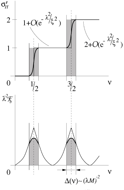
Figure 6: Finite size scaling of the Hall conductance $\sigma^{\prime}_{H}$ and the bulk free energy $\mathcal{F}_{b}/\lambda^{2}$ with varying $\nu$. The dark areas at $\nu=1/2,~{}3/2$  etc. indicate the critical regimes $\Delta(\nu)\propto\lambda^{-2}$ where $\sigma^{\prime}_{H}$ varies smoothly from one plateau value to the next. Similarly, the “cusp” in $\mathcal{F}_{b}/\lambda^{2}$ is smoothed out due to the finite scale size $\lambda$, see text.

6.2 $\vartheta$ renormalization

From Eqs (67) and (78) we obtain the $\beta$ functions (see also Fig. 7)

$$\beta_{\sigma}(\sigma^{\prime}) = \frac{d\sigma^{\prime}}{d\ln\lambda}=\sigma^{\prime}\ln\sigma^{\prime}$$ (81)

$$\beta_{\theta}(\theta^{\prime}) = \frac{d\theta^{\prime}}{d\ln\lambda}=\frac{\theta^{\prime}}{\pi}\Bigl{[}2\pi-|\theta^{\prime}|\Bigr{]}\ln\Bigl{[}\frac{|\theta^{\prime}|}{2\pi-|\theta^{\prime}|}\Bigr{]}$$ (82)

which are amongst the most important results of this paper. Eqs (81) and (82) together with the weak coupling instanton results of Section 4.2 give rise to the renormalization group flow lines of Fig. 4. We identify two different kinds of strong coupling fixed points, a massive one at $\sigma^{\prime}=\theta^{\prime}=0$ and a critical one at $\sigma^{\prime}=0$ and $\theta^{\prime}=\pm\pi$. Near $\theta^{\prime}=0$ we have

$$\beta_{\sigma}=\beta_{\sigma}(\sigma^{\prime})=\sigma^{\prime}\ln\sigma^{\prime}~{},~{}~{}\beta_{\theta}=\beta_{\theta}(\theta^{\prime})=2{\theta^{\prime}}\ln|\theta^{\prime}|$$ (83)

indicating that the Hall conductance is robustly quantized. Near $\theta^{\prime}=\pi$ for $\sigma^{\prime}=0$ we find

$$\frac{d(\pi-\theta^{\prime})}{d\ln\lambda}=2(\pi-\theta^{\prime}).$$ (84)

The exponent value $2$ is the inverse of the correlation length exponent given by Eq. (80) and, at the same time, a standard result for a first order phase transition in two dimensions.

Figure 7: The function $\beta_{\theta}$ with varying $\theta^{\prime}$, see text.

6.3 Conductance distributions

A very interesting feature of the large $N$ expansion is that $Z[q]$ near the plateau transition can be evaluated exactly and not just to lowest orders in a series expansion in $\mathcal{C}[q]$. The exact result is most conveniently expressed in terms of the Hall conductance $\sigma_{H}^{\prime}(\lambda)=k(\nu)+\frac{\theta^{\prime}(\lambda)}{2\pi}$. Let $\nu\approx k_{0}+\frac{1}{2}$ denote the transition regime with $k_{0}$ an arbitrary integer. We then obtain

$$Z[q]=e^{-\mathcal{F}_{b}}\times\left\{(1+k_{0}-\sigma_{H}^{\prime})e^{2\pi ik_{0}\mathcal{C}[q]}+(\sigma_{H}^{\prime}-k_{0})e^{2\pi i(k_{0}+1)\mathcal{C}[q]}\right\}~{}$$ (85)

where

$$\sigma_{H}^{\prime}=\sigma_{H}^{\prime}(\lambda)=k_{0}+\frac{1}{2}e^{\lambda^{2}M^{2}\Delta\nu}\cosh^{-1}(\lambda^{2}M^{2}\Delta\nu)~{}~{},~{}~{}~{}\Delta\nu=\nu-k_{0}-\frac{1}{2}.$$ (86)

Notice that Eq. (86) varies continuously from one plateau value ($k_{0}$) to the next ($k_{0}+1$) as the relative filling fraction $\Delta\nu$ varies from negative to positive values, see Fig. 6. On the other hand, Eq. (85) describes this transition in terms of a probability distribution of the quantum Hall states $k_{0}$ and $k_{0}+1$ that are represented by the phase factors $e^{2\pi k_{0}i\mathcal{C}[q]}$ and $e^{2\pi(k_{0}+1)i\mathcal{C}[q]}$ respectively.

In order to see that Eq. (85) actually defines a distribution of the fractional part $\theta^{\prime}(\lambda)$ of the Hall conductance we introduce the set of variables

$$\theta_{n}=2\pi(k_{0}-k(\nu)+n)$$ (87)

with $n=0,1$. The bulk part $Z_{b}[q]$ in Eq. (85) can now be written as a sum

$$Z_{b}[q]=e^{-\mathcal{F}_{b}}\times\sum_{n=0}^{1}P_{n}~{}e^{i\theta_{n}\mathcal{C}[q]}.$$ (88)

Here, $P_{n}=P_{n}(\theta^{\prime}(\lambda))$ is a normalized weight

$$\sum_{n=0}^{1}P_{n}=1~{},~{}~{}~{}\left(P_{0},~{}P_{1}\right)=\left(1+\frac{\theta_{0}-\theta^{\prime}(\lambda)}{2\pi},1-\frac{\theta_{1}-\theta^{\prime}(\lambda)}{2\pi}\right)$$ (89)

and the expectations are denoted by

$$\langle\theta^{k}\rangle=\sum_{n=0}^{1}P_{n}\theta^{k}_{n}~{},~{}~{}\langle\theta\rangle=\theta^{\prime}(\lambda).$$ (90)

These results indicate that the bulk quantity $\theta^{\prime}(\lambda)$ is actually broadly distributed in a highly non-gaussian manner. For example, we can express Eq. (88) in terms of a cumulant expansion

$$\ln Z_{b}[q]=-\mathcal{F}_{b}+\tilde{S}_{\sigma}^{\prime}[q]$$ (91)

where

$$\tilde{S}_{\sigma}^{\prime}[q]=i\theta^{\prime}(\lambda)\mathcal{C}[q]-\frac{1}{2\mathcal{!}}\zeta_{2}^{\prime}(\lambda)\mathcal{C}^{2}[q]-\frac{i}{3\mathcal{!}}\zeta_{3}^{\prime}(\lambda)\mathcal{C}^{3}[q]+\mathcal{O}(\mathcal{C}^{4}).$$ (92)

The higher order cumulants multiplying $\mathcal{C}^{2}[q]$, $\mathcal{C}^{3}[q]$ etc. can all be expressed in terms of the “averaged” quantity $\langle\theta\rangle=\theta^{\prime}(\lambda)$. For example

$$\zeta_{2}^{\prime}(\lambda)=\langle\theta^{2}\rangle-\langle\theta\rangle^{2}=|\theta^{\prime}(\lambda)|(2\pi-|\theta^{\prime}(\lambda)|).$$ (93)

Notice that as one approaches the transition $\theta^{\prime}(\lambda)\rightarrow\pi$ the “root mean square fluctuation” $\sqrt{\zeta_{2}^{\prime}(\lambda)}$ becomes equal to the averaged value $\pi$. Away from the transition both the averaged value $\theta^{\prime}(\lambda)$ and the higher order cumulants $\zeta^{\prime}(\lambda)$ become exponentially small in $\lambda$. The large $N$ expansion is therefore a prototypical example of the broad “mesoscopic conductance distributions” that are of interest in the quantum theory of metals. [36] Distributions like Eq. (89) do not affect the scaling behavior of the system, however, since this behavior depends on the “ensemble averaged” quantity $\theta^{\prime}(\lambda)$ alone.

6.4 Twisted boundary conditions

In the original papers in the field [7] it was already argued on general grounds that de-localized or extended “bulk” excitations at $\theta(\nu)=\pm\pi$ must generally exist for all values $M,N\geq 0$. The idea naturally emerges from ’t Hooft’s duality argument that is based on the response of the system to imposing twisted boundary conditions. The effect of these boundary conditions is obtained by inserting $\mathcal{C}[q]=\frac{1}{2}$ in Eq. (88). We can write

$$-\ln Z_{b}[q]=\mathcal{F}_{b}-\ln\sum_{n=0}^{1}P_{n}(\theta^{\prime})~{}e^{i\theta_{n}/2}=\mathcal{F}_{b}+\Delta\mathcal{F}.$$ (94)

The shift $\Delta\mathcal{F}$ in the free energy due to twisted boundary conditions can be expressed in terms of $\theta^{\prime}$ defined in Eq. (78) and the result is

$$\Delta\mathcal{F}(\theta^{\prime})=-\ln\left(1-\frac{|\theta^{\prime}|}{\pi}\right).$$ (95)

As long as $\theta(\nu)$ is different from $\pm\pi$ the shift $\Delta\mathcal{F}$ is exponentially small in the scale size $\lambda$ indicating that the system has a mass gap. However, when $\theta(\nu)$ approaches $\pm\pi$ the response $\Delta\mathcal{F}\propto\ln\xi$ diverges which means that the system now has gapless “bulk” excitations. Notice that these findings are entirely consistent with all the other ideas and results that have been discussed sofar, in particular Coleman’s picture of dissociating charges at $\theta(\nu)=\pm\pi$, the scaling functions describing the quantum Hall plateau transitions as well as the statistics of conductance distributions addressed in the previous section.

In a subsequent paper we will embark on the critical correlations of the large $N$ theory and show that they map onto the one dimensional Ising model at zero temperature. [37] This is unlike the grassmannian theory with $0\leq M,N\lesssim 1$ where, as well is known, the transition is a second order one with exponents that vary continuously with varying $M$ and $N$. [12] Despite these and many other differences, the basic phenomena of de-localization and scaling, including the robust quantization of the Hall conductance, are nevertheless the same.

7 Pseudo instanton phase ${12\pi\lambda^{2}M_{0}^{2}}/{N}\ll 1$ and cross-over

We have now completed the strong coupling quantum Hall side of the large $N$ expansion. In this Section we embark on the problem of cross-over between the weak coupling instanton phase discussed in Section 4 and the strong coupling results of the previous Section. For this purpose we consider Eqs (68) and (69) in the regime where the dimensionless quantity ${12\pi\lambda^{2}M_{0}^{2}}/{N}$ is small. To obtain a rapidly converging series we simply perform the integral over the auxiliary field $\eta$ such that the theory be written as sum over integral topological sectors $n$

$$Z[q] = e^{2\pi ik(\nu)\mathcal{C}[q]}Z_{b}[q]$$

$$Z_{b}[q] = \sum_{n}\exp\left\{-\kappa(\lambda)(n+\mathcal{C}[q])^{2}+i\theta(\nu)(n+\mathcal{C}[q])\right\}.$$ (96)

where

$$\kappa(\lambda)=\frac{\pi N}{12\lambda^{2}M_{0}^{2}}\gg 1.$$ (97)

Notice that there exists a large regime in $\lambda$ where the sum over $n$ is rapidly converging and, at the same time, the condition for strong coupling $\lambda M_{0}\gg 1$ is satisfied. In terms of the scaling parameter $\sigma(\lambda)$ or $\sigma^{\prime}(\lambda)$ we can write

$$e^{-\sqrt{12N/\pi}}\ll\sigma(\lambda)=\sigma^{\prime}(\lambda)=e^{-\lambda M_{0}}\ll 1.$$ (98)

We term this regime the pseudo instanton phase because Eq. (96) defines a trigonometric series in $\theta(\nu)$ which is in many ways similar to the one obtained from the semiclassical theory based on instantons (Section 4). By expanding Eq. (96) in powers of $\mathcal{C}[q]$ we obtain the same general form as before

$$\ln Z_{b}[q]=-\mathcal{F}_{b}+i\theta^{\prime}~{}\mathcal{C}[q]+\dots$$ (99)

In what follows we separately consider the free energy $\mathcal{F}_{b}$ (Section 7.1) and the observable theory $\theta^{\prime}$ (Section 7.2) respectively.

7.1 Free energy

The free energy can be expressed in the general form of Eq. (30)

$$\lambda^{2}{\mathcal{F}_{b}}=-\frac{24M_{0}^{2}}{\pi N}\sum_{n=0}^{\infty}\phi_{n}(\kappa)\cos n\theta(\nu).$$ (100)

Here, the functions $\phi_{n}(\kappa)$ to lowest orders in $n$ are computed to be

$$~{}~{}~{}~{}~{}~{}~{}~{}~{}~{}~{}~{}~{}~{}~{}~{}~{}~{}~{}~{}~{}~{}~{}\phi_{0}(\kappa) = -\frac{1}{2}\kappa e^{-2\kappa}+\mathcal{O}(e^{-4\kappa})$$

$$\phi_{1}(\kappa) = ~{}~{}~{}~{}\kappa e^{-\kappa}~{}~{}+\mathcal{O}(e^{-3\kappa})$$

$$\phi_{2}(\kappa) = -\frac{1}{4}\kappa e^{-2\kappa}+\mathcal{O}(e^{-4\kappa}).$$ (101)

More generally one finds the dominating behavior $\phi_{n}(\kappa)\simeq e^{-n\kappa}$ for $n>0$. By expressing $\kappa$ in terms of $\sigma$ given in Eq. (98) one can write this result as $\phi_{n}(\kappa)\simeq\left[\exp\{-\frac{\pi}{12\ln^{2}\sigma}\}\right]^{nN}$. This behavior is reminiscent of the instanton factors $W^{nN}(\sigma)$ found in the weak coupling regime (Section 4).

7.1.1 Relation to quantum Hall phase

Let us first establish the contact with the quantum Hall phase. For this purpose we go back to the result of Eq. (75) which is the $\lambda=\infty$ limit of the free energy. This result can be expanded in terms of a trigonometric series according to

$$~{}~{}~{}~{}~{}~{}~{}~{}~{}~{}~{}~{}~{}~{}~{}~{}~{}~{}~{}\lambda^{-2}{\mathcal{F}_{b}} = ~{}~{}~{}\frac{3M_{0}^{2}}{\pi N}~{}\theta^{2}(\nu)$$ (102)

$$= -\frac{24M_{0}^{2}}{\pi N}\sum_{n=0}^{\infty}\phi_{n}(0)\cos n\theta(\nu).$$

The coefficients $\phi_{n}(0)$ are defined by

$$\phi_{n}(0) = -\frac{1}{8\pi}\int_{-\pi}^{\pi}\vartheta^{2}\cos(n\vartheta){d\vartheta}=(-1)^{n+1}\frac{1}{2n^{2}},\qquad n>0$$ (103)

$$\phi_{0}(0) = -\frac{1}{16\pi}\int_{-\pi}^{\pi}\vartheta^{2}{d\vartheta}=-\frac{\pi^{2}}{24}.$$ (104)

It is clear that the coefficients $\phi_{n}(0)$ in Eq. (102) are the $\kappa=0$ limit of the functions $\phi_{n}(\kappa)$ in Eq. (100). Eq. (102) is retained also if one takes the finite size scaling corrections into account, see Fig.6. The only difference is that the coefficients $\phi_{n}(0)$ in Eq. (102) are replaced by a series in powers of $\kappa$.

Figure 8: The function $\phi_{1}(\kappa)$ with varying $\kappa$, see text.

As a typical example of the cross-over between the quantum Hall and pseudo instanton phases we consider the function $\phi_{1}(\kappa)$. A detailed investigation of this function in the quantum Hall phase shows that the series expansion in $\kappa$ is of the form

$$\phi_{1}(\kappa) = \frac{1}{2}+\sum_{s=1}^{\infty}a_{s}\kappa^{2s}~{};~{}~{}~{}~{}~{}~{}~{}~{}~{}\kappa\ll 1$$ (105)

where the lowest order coefficient $a_{1}$ in the series is negative. On the other hand, from Eq. (101) we obtain the result for the pseudo instanton phase

$$\phi_{1}(\kappa) = \kappa e^{-\kappa}~{};~{}~{}~{}~{}~{}~{}~{}~{}~{}~{}~{}~{}~{}~{}~{}~{}~{}~{}~{}~{}\kappa\gg 1$$ (106)

From Eqs (105) and (106) we infer that $\phi_{1}(\kappa)$ can in general be written as the product of an algebraic part $v_{1}(\kappa)$ and an exponential part $e^{-\kappa}$

$$\phi_{1}(\kappa)=v_{1}(\kappa)e^{-\kappa}.$$ (107)

For the purpose of illustration we employ the following trial function that satisfies the asymptotic constraints of Eqs (105) and (106)

$$\phi_{1}(\kappa)=\frac{1}{2}\sqrt{1+\kappa^{2}}\exp\left\{-\sqrt{1+\kappa^{2}}+1\right\}.$$ (108)

This function along with the asymptotic behavior of Eqs (105) and (106) is plotted in Fig. 8. Eq. (108) determines the function $v_{1}(\kappa)$ in Eq. (107) to be

$$v_{1}(\kappa)=\frac{1}{2}\sqrt{1+\kappa^{2}}\exp\left\{-\sqrt{1+\kappa^{2}}+1+\kappa\right\}.$$ (109)

This function is algebraic in the sense that it smoothly interpolates between $v_{1}=\frac{1}{2}$ for small $\kappa$ and $v_{1}\propto\kappa$ for large values of $\kappa$.

7.1.2 Relation to instanton phase

Like the dilute instanton gas result discussed in Section 4.1, the free energy of the pseudo instanton phase is dominated by the $n=1$ term in Eqs (100) and (101). Given the general form of $\phi_{1}(\kappa)$ in the strong coupling phase, Eq. (107), it is not difficult to cast this term in the typical form of the dilute instanton gas. More specifically, let $\lambda^{\prime}$ denote the system size then we can write the result as an integral over scale $\lambda$ as follows

$$~{}~{}~{}~{}~{}~{}~{}~{}~{}~{}~{}~{}~{}~{}~{}~{}~{}{(\lambda^{\prime})^{-2}}{\mathcal{F}_{b}} \approx -\frac{24M_{0}^{2}}{\pi N}\phi_{1}(\kappa(\lambda^{\prime}))\cos\theta(\nu)$$ (110)

$$= ~{}-\int_{0}^{\lambda^{\prime}}\frac{d\lambda}{\lambda^{3}}~{}~{}w(\lambda)W^{N}(\lambda)\cos\theta(\nu)~{}~{}~{}~{}$$

where the functions $w$ and $W$ are given by

$$w(\lambda)=4\left(\frac{dv_{1}(\kappa)}{d\kappa}-v_{1}(\kappa)\right)~{},~{}~{}W(\lambda)=\exp(-\frac{\pi}{12\lambda^{2}M_{0}^{2}})$$ (111)

with $v_{1}(\kappa)$ an algebraic function of $\kappa=\kappa(\lambda)$.

Figure 9: The function $W(\sigma)$ with varying $\sigma$ describing the cross-over between and the dilute instanton gas at $\sigma\rightarrow\infty$ and the quantum Hall phase at $\sigma\rightarrow 0$. The two different branches are the weak coupling instanton result of Eq. (37) and the strong coupling result of Eq. (112) respectively, see text.

The contact with the instanton result of Eq. (37) is complete if we express the functions $W(\lambda)$ and $w(\lambda)$ in terms of the scaling parameter $\sigma(\lambda)=e^{-\lambda M_{0}}\ll 1$ rather than the scale size $\lambda$. The strong coupling expressions for the $w(\sigma)$ and $W(\sigma)$ functions read

$$w(\sigma)=4\left(\frac{dv_{1}(\kappa(\sigma))}{d\kappa(\sigma)}-v_{1}(\kappa(\sigma))\right)~{},~{}~{}W(\sigma)=\exp(-\frac{\pi}{12\ln^{2}\sigma})~{},~{}~{}\sigma\ll 1$$ (112)

where $\kappa(\sigma)={\pi N}/{12\ln^{2}\sigma}$.

7.1.3 Instantons regained

In conclusion, the large $N$ steepest descend methodology and the semiclassical instanton methodology are complementary descriptions that together elucidate the complete structure of the $\vartheta$ vacuum. We find, in particular, that semiclassical concepts like the “dilute instanton gas” and “discrete topological sectors” have a universal significance that extends all the way down to the strong coupling phase of the large $N$ expansion. By comparing Eqs (112) and (37), for example, one sees that the cross-over between the weak and strong coupling phases is primarily controlled by a single, $N$-independent function $W(\sigma)$. This function is monotonically decreasing from unity to zero as $\sigma$ increases from zero to infinity, see Fig. 9. On the other hand, the results of Eqs (109) and (111) clearly show that main task of the $w(\sigma)$ function is to correctly describe the cross-over from the pseudo instanton phase to the strong coupling quantum Hall phase where the factor $W^{N}$ in Eq. (110) is close to unity. Generally speaking, however, the $w(\sigma)$ function is a $1/N$ correction relative to $W(\sigma)$ and therefore of secondary importance.

The results for the $W(\sigma)$ function plotted in Fig. 9 furthermore indicate that the semiclassical theory of instantons described by Eq. (37) is only valid in the range $\sigma\gtrsim 1$ or $\lambda M_{0}\lesssim 1$ as expected. Upon entering the strong coupling phase the functions $W(\sigma)$ and $w(\sigma)$ generally have a different meaning which cannot be obtained from semiclassical arguments alone. The important conclusion to be drawn from the present analysis is that the thermodynamic limit of the dilute instanton gas truly exists and is finite.

7.2 Physical observables

Next, we embark on the observable quantity $\theta^{\prime}$ defined in Eq. (99). By taking only the lowest order terms $n=0,\pm 1$ in Eq. (96) into account we obtain

$$\theta^{\prime}(\lambda) = \theta(\nu)~{}~{}-4\kappa(\lambda)e^{-\kappa(\lambda)}\sin\theta(\nu).$$ (113)

By substituting $\sigma^{\prime}=\sigma^{\prime}(\lambda)=e^{-\lambda M_{0}}$ for $\kappa(\lambda)$ we obtain the following renormalization group equations for the pseudo instanton phase

$$\beta_{\sigma} = \frac{d\sigma^{\prime}}{d\ln\lambda}=\sigma^{\prime}\ln\sigma^{\prime}$$ (114)

$$\beta_{\theta} = \frac{d\theta^{\prime}}{d\ln\lambda}=-g_{1}(\sigma^{\prime})W^{N}(\sigma^{\prime})\sin\theta^{\prime}$$ (115)

where the $W(\sigma^{\prime})$ function is the same as in Eq. (112) and

$$g_{1}(\sigma^{\prime})=8\left(\frac{\pi N}{12\ln^{2}\sigma^{\prime}}\right)\left[\frac{\pi N}{12\ln^{2}\sigma^{\prime}}-1\right],~{}~{}~{}~{}~{}~{}e^{-\sqrt{12N/\pi}}\ll\sigma^{\prime}\ll 1.$$ (116)

7.2.1 Relation to instanton phase

These expressions are of the same general form as the instanton results of Eqs (40) and (41) that are valid in the range $\sigma^{\prime}\gg 1$. It is easy to see, for example, that the higher order terms in Eq. (115) are all of the same type as the weak coupling results described in Eqs (44) and (45). Unlike Eq. (43), however, our results for the observable $\sigma^{\prime}$ or the function $\beta_{\sigma}$ do not display any dependence on $\theta^{\prime}$. The reason being that in the definition of $\delta S$ in Eq. (63) we have neglected all the terms that couple the $q$ matrix field and the $A_{\mu}$ vector field. It can be shown that a more careful definition of the quantity $g^{\prime}$ or $\sigma^{\prime}$ generally leads to the same geometrical series for the $\beta_{\sigma}$ function as in Eqs (43) and (45). [37] In the regime of interest the $\theta^{\prime}$ dependent terms in the $\beta_{\sigma}$ function are all insignificant relative to the leading order result of Eq. (115), however, and they do not alter the main conclusions of the present investigation.

$n$	$\beta_{\theta}^{(n)}(0)$
$1$	$-2.794$
$2$	$-0.633$
$3$	$-0.268$
$4$	$-0.146$
⋮	⋮
$n$	$-\frac{2}{\pi n^{2}}$

Table 1: Numerical values of $\beta_{\theta}^{(n)}(0)$, see text.

7.2.2 Relation to quantum Hall phase

Keeping these remarks in mind we next turn to the renormalization group results obtained for the quantum Hall phase, Eqs (81) and (82). We expand the latter in a trigonometric series according to

$$\beta_{\theta}(\theta^{\prime}) = \frac{\theta^{\prime}}{\pi}\Bigl{[}2\pi-|\theta^{\prime}|\Bigr{]}\ln\Bigl{[}\frac{|\theta^{\prime}|}{2\pi-|\theta^{\prime}|}\Bigr{]}=~{}\sum_{n=1}^{\infty}\beta_{\theta}^{(n)}(0)~{}\sin n\theta^{\prime}.$$ (117)

The coefficients $\beta_{\theta}^{(n)}(0)$ are finite numbers defined by

$$\beta_{\theta}^{(n)}(0)=\int_{-\pi}^{\pi}\frac{d\vartheta}{\pi}\sin(n\vartheta)\beta_{\theta}(\vartheta).$$ (118)

These results clearly show that the instanton functions $\beta_{\theta}^{(n)}(\sigma^{\prime})$ in Eq. (44) all have a well defined strong coupling limit $\sigma^{\prime}=0$. In the same limit we find that all the coefficients $\beta_{\sigma}^{(n)}(\sigma^{\prime})$ in Eq. (43) are zero as expected.

In Table 1 we list the numerical values of the lowest order coefficients $\beta_{\theta}^{(n)}(0)$. By truncating the series in Eq. (117) one generally retains the correct fixed point structure of the theory. The exact exponent value $2$ in Eq. (84) is expanded in an infinite series according to

$$2=\sum_{n=1}^{\infty}n(-1)^{n}\beta_{\theta}^{(n)}(0).$$ (119)

By keeping only the lowest order term we obtain an approximate exponent value of $2.8$ which in all respects is quite reasonable. The renormalization behavior is therefore well represented if one extends Eqs (114) and (115) to include the $n=1$ sector of the quantum Hall phase according to

$$g_{1}(\sigma^{\prime})\approx\beta_{\theta}^{(1)}(0)=2.794\dots,~{}~{}~{}~{}~{}~{}~{}\sigma^{\prime}\ll e^{-\sqrt{12N/\pi}}.$$ (120)

Notice that the results for the combination $g_{1}(\sigma^{\prime})W^{N}(\sigma^{\prime})$ in Eq. (115) are quite similar to those of the quantity $\phi_{1}(\kappa)=v_{1}(\kappa)e^{-\kappa}$ of the free energy, Eq. (107). Fig. 8 illustrates the cross-over behavior of the present case as well.

8 Summary and conclusion

	Quantum Hall phase	Pseudo instanton phase	Instanton phase
$\sigma^{\prime}=\sigma^{\prime}(\lambda)$	$\displaystyle 0\leq\sigma^{\prime}\ll e^{-\sqrt{12N/\pi}}$	$\displaystyle e^{-\sqrt{12N/\pi}}\ll\sigma^{\prime}\ll 1$	$\displaystyle 1\ll\sigma^{\prime}$
$W(\sigma^{\prime})$	$\displaystyle e^{-\pi/(12\ln^{2}\sigma^{\prime})}$	$\displaystyle e^{-\pi/(12\ln^{2}\sigma^{\prime})}$	$\displaystyle 4\pi e^{-\gamma-1/2}\sigma e^{-2\pi\sigma^{\prime}}$
$f(\sigma^{\prime})$	$\displaystyle\sigma^{\prime}\ln\sigma^{\prime}$	$\displaystyle\sigma^{\prime}\ln\sigma^{\prime}$	$\displaystyle-\frac{1}{2\pi}$
$f_{1}(\sigma^{\prime})$	-	-	$\displaystyle{8(2\pi)^{1/2}e^{-1}N^{3/2}}(\sigma^{\prime})^{2}$
$g_{1}(\sigma^{\prime})$	$\displaystyle 2.794\dots$	$\displaystyle 8\left(\frac{\pi N}{12\ln^{2}\sigma^{\prime}}\right)\left[\frac{\pi N}{12\ln^{2}\sigma^{\prime}}-1\right]$	$\displaystyle 8(2\pi)^{3/2}e^{-1}N^{5/2}(\sigma^{\prime})^{2}$

Table 2: Generalized instanton results for the renormalization group $\beta$ functions $\beta_{\sigma}=f(\sigma^{\prime})-f_{1}(\sigma^{\prime})W^{N}(\sigma^{\prime})\cos\theta^{\prime}$ and $\beta_{\theta}=-g_{1}(\sigma^{\prime})W^{N}(\sigma^{\prime})\sin\theta^{\prime}$ describing the entire regime $0\leq\sigma^{\prime}<\infty$. An estimate for the function $f_{1}(\sigma^{\prime})$ in the pseudo instanton phase and the quantum Hall phase is beyond the scope of the present investigation, see text.

In this investigation we have addressed the super universality concept of the $\vartheta$ vacuum in the large $N$ expansion of the $CP^{N-1}$ model. This has been done in three consecutive steps. First, we study the general consequences of “massless chiral edge excitations” in the context of the grassmannian $SU(M+N)/S(U(M)\times U(N))$ non linear sigma model. By separating the fractional topological sectors from the integral ones we obtain a general theory of massless edge excitations together with the fundamental parameters (“physical observables” or “conductances”) that define the renormalization behavior of the $\vartheta$ vacuum. Secondly, we explicitly evaluate these parameters employing a revised and adapted version of the usual large $N$ steepest descend methodology. This leads to a demonstration of the robust quantization of the Hall conductance along with exact scaling results for the quantum Hall plateau transitions. Thirdly, we employ the results recently obtained from instantons in order to bridge the gap between the weak and strong coupling sides of the large $N$ expansion. The most general way in which the renormalization group $\beta$ functions can be expressed is in terms of discrete topological sectors $n$ according to

$$\beta_{\sigma}(\sigma^{\prime},\theta^{\prime}) = \sum_{n=0}^{\infty}\beta_{\sigma}^{(n)}(\sigma^{\prime})\cos n\theta^{\prime}\approx f(\sigma^{\prime})-f_{1}(\sigma^{\prime})W^{N}(\sigma^{\prime})\cos\theta^{\prime}$$ (121)

$$\beta_{\theta}(\sigma^{\prime},\theta^{\prime}) = \sum_{n=1}^{\infty}\beta_{\theta}^{(n)}(\sigma^{\prime})\sin n\theta^{\prime}\approx~{}~{}~{}~{}~{}~{}~{}~{}-g_{1}(\sigma^{\prime})W^{N}(\sigma^{\prime})\sin\theta^{\prime}$$ (122)

We have shown that by retaining only the lowest order terms in the series the renormalization is well represented in the entire range $0\leq\sigma^{\prime}<\infty$. In Table 2 we list the generalized instanton functions $W(\sigma^{\prime})$, $f(\sigma^{\prime})$, $f_{1}(\sigma^{\prime})$ and $g_{1}(\sigma^{\prime})$ obtained in the three different regimes that we have considered. These results, together with the exact strong coupling expressions of Eqs (81) and (82), are the justification for the renormalization group flow lines sketched in Fig. 4.

It should be mentioned that our findings are in complete accordance with the original work of Jevicki [33] who showed that the large $N$ steepest descend methodology and the instanton methodology are formally the same. Our results invalidate the historical “large $N$ picture” of the $\vartheta$ vacuum, however, in particular the claims which say that “discrete topological sectors” do not exist and “instantons” are irrelevant.[21, 22] These historical claims are borne out of a mishandling of the massless chiral edge excitations in the problem, as well as incorrect assumptions about the order in which the thermodynamic limit and the large $N$ limit should in general be taken.

Even though the idea of super universality of quantum Hall physics has already been foreshadowed by the pioneering papers in the field more than two decades ago, [7] over the years this idea has nevertheless been confronted with many incorrect expectations and conjectures [24, 25, 26, 27, 28] that in one way or the other are all related to the historical “large $N$ picture” of the $\vartheta$ angle. There is, for example, the persistent belief in the literature which says that the theory generally has no gapless excitations, not even at $\vartheta=\pi$, and the quantum Hall effect somehow does not truly exist. By demonstrating super universality as done in the present investigation, we essentially establish a new paradigm for our understanding of topological issues in quantum field theory in general, and the experiment on the quantum Hall effect in particular.

9 Acknowledgements

The author has benefitted from stimulating discussions with A. Abanov, I.S. Burmistrov and A.M. Finkelstein. The research was funded in part by the Dutch Science Foundations NWO and FOM and the EU-Transnational Access program (RITA-CT 2003-506095).

References

- [1] A.M.M. Pruisken, M.A. Baranov and B. Škorić, Phys. Rev. B60, 16807 (1999)
- [2] A.M.M. Pruisken, B. Škorić and M. Baranov, Phys. Rev. B60, 16838 (1999)
- [3] B. Škorić and A.M.M. Pruisken, Nucl. Phys. B559, 637 (1999)
- [4] A.M.M. Pruisken, R. Shankar, Naveen Surendran Phys. Rev. B72, 035329 (2005)
- [5] A.M.M. Pruisken, R. Shankar, Naveen Surendran, Europhys. Lett. 82, 47005 (2008)
- [6] F.D.M. Haldane, Phys. Lett. A93 464 (1983), Phys. Rev. Lett. 50 1153 (1983)
- [7] A.M.M. Pruisken, Nucl. Phys. B235 277 (1984), H. Levine, S. Libby and A.M.M. Pruisken, Phys. Rev. Lett. 51, 20 (1983), Nucl. Phys. B240 [FS12] 30, 49, 71 (1984)
- [8] R.E. Prange in The Quantum Hall Effect, Eds R.E. Prange and S.M. Girvin, (Berlin, Springer, 1990)
- [9] See e.g. R.T.F. van Schaijk, A. de Visser, S.M. Olsthorn, H.P. Wei and A.M.M. Pruisken, Phys. Rev. Lett. 84,1567 (2000)
- [10] X.G. Wen, Phys. Rev. B41 12838 (1990), Int. J. Mod. Phys. B6 1711 (1991), cond-mat/9506066 (unpublished)
- [11] See e.g. R. Rajaraman, Instantons and solitons, (Amsterdam, North-Holland, 1982); A.M. Polyakov, Gauge fields and strings, (Harwood Academic Publishers, Shur, 1987)
- [12] A.M.M. Pruisken and I.S. Burmistrov, Ann. Phys. 316 285 (2005)
- [13] A.M.M. Pruisken and I.S. Burmistrov, Ann. Phys. 322 1265 (2007), Pis’ma v ZhETF v. 87, 252 (2008)
- [14] I.S. Burmistrov and A.M.M. Pruisken, Phys. Rev. Lett. 101, 056801 (2008)
- [15] E. Brézin, S. Hikami and J. Zinn-Justin, Nucl. Phys. B165, 528 (1980)
- [16] M.A. Baranov, A.M.M. Pruisken and B. Škorić, Phys. Rev. B60, 16821 (1999), B66, 075317 (2002)
- [17] A.M.M. Pruisken, Phys. Rev. Lett. 61, 1297 (1988)
- [18] H.P. Wei, D.C. Tsui and A.M.M. Pruisken, Phys. Rev. B33, 1488 (1986); H.P. Wei, D.C. Tsui, M.A. Palaanen and A.M.M. Pruisken, Phys. Rev. Lett. 61, 1294 (1988). For recent advances see W. Li, G.A. Csáthy, D.C. Tsui, L.N. Pfeiffer and K.W. West, Phys. Rev. Lett. 94, 206807 (2005); A.M.M. Pruisken, D.T.N. de Lang, L.A. Ponomarenko and A. de Visser, Solid State Commun. 137, 540 (2006)
- [19] V. Ambegaokar, U. Eckern and G. Schön, Phys. Rev. Lett. 48, 1745 (1982), G. Schön and A.D. Zaikin, Phys. Rep. 198, 237 (1990)
- [20] A. D’Adda, P. Di Vecchia and M. Luescher, Nucl. Phys. B146, 63 (1978)
- [21] E. Witten, Nucl. Phys. B149, 285 (1979)
- [22] I. Affleck, Nucl. Phys. B162, 461 (1980): B171, 420 (1980)
- [23] S. Coleman, Aspects of Symmetry, (University Press, Cambridge, 1989)
- [24] I. Affleck, J. Phys. C16 5839 (1983), Nucl. Phys. B257 397 (1985), B265 409 (1986), B305 582 (1988), Phys. Rev. Lett. 56 746 (1986)
- [25] I. Affleck, Phys. Rev. Lett. 66, 2429 (1991)
- [26] J.J.J.M Verbaarschot and M.R. Zirnbauer, J. Phys. A17 1093 (1985)
- [27] H.A. Weidenmueller, Nucl. Phys. B290 87 (1987)
- [28] M.R. Zirnbauer, Ann. d. Physik 3 513 (1994), J. Math. Phys. 38 2007 (1997), cond-matt/9903338 (unpublished)
- [29] A.M.M. Pruisken in The Quantum Hall Effect, Eds R.E. Prange and S.M. Girvin, (Berlin, Springer, 1990)
- [30] A.M.M. Pruisken, Phys. Rev. B31 416 (1985)
- [31] A.M.M. Pruisken, Nucl. Phys. B285 719 (1987), B290 61 (1987)
- [32] B. Berg and M. Lüsher, Commun. Math. Phys. 69 57 (1979); V. A. Fateev, I.V. Frolov and A.S. Schwartz Nucl. Phys. B154 1 (1979)
- [33] A. Jevicki, Phys. Rev. D20, 3331 (1979)
- [34] A.M.M. Pruisken, Nucl. Phys. B295 653 (1988)
- [35] S. Coleman, Ann. of Phys. 101, 239 (1976)
- [36] B.L. Altshuler, V.E. Kravtsov and I.V. Lerner, Zh. Eksp. Teor. Fiz. 91, 2276 (1986) [Sov. Phys. JETP 64, 1352 (1986)]; M.H. Cohen and A.M.M. Pruisken, Phys. Rev. B49, 4593 (1994) and references therein.
- [37] A.M.M. Pruisken, I.S. Burmistrov and S. Shankar, cond-mat/0602653 (unpublished)