Alignment of galaxy spins in the vicinity of voids

Abstract

We provide limits on the alignment of galaxy orientations with the direction to the void center for galaxies lying near the edges of voids. We locate spherical voids in volume limited samples of galaxies from the Sloan Digital Sky Survey using the HB inspired void finder and investigate the orientation of (color selected) spiral galaxies that are nearly edge-on or face-on. In contrast with previous literature, we find no statistical evidence for departure from random orientations. Expressed in terms of the parameter $c$, introduced by Lee & Pen to describe the strength of such an alignment, we find that $c<0.11(0.13)$ at 95% (99.7%) confidence limit within a context of a toy model that assumes a perfectly spherical voids with sharp boundaries.

I Introduction

Within the currently accepted paradigm for structure formation, galaxies form through a complex series of mergers and accretion events in a beaded filamentary network of dark matter halos and subhalos. The cooling and condensation of gas within these dark matter hosts leads to the visible signatures by which we recognize galaxies Rees and Ostriker (1977); Silk (1977); White and Rees (1978); Fall and Efstathiou (1980); Blumenthal et al. (1984). While this broad picture has received impressive support in recent years, many of the detailed processes remain poorly understood. In particular the manner in which feedback alters the rate at which gas cools and the coupling between the angular momentum of the gas and the dark matter – both of which effect the sizes and shapes of disks – are outstanding problems in galaxy formation. We still cannot form realistic looking disk galaxies from an ab initio simulation in a cosmological context.

This lack is important not just for our understanding of galaxy formation, but also because it impacts upon one of the most important probes of structure formation and cosmology: weak gravitational lensing (see Schneider (2006) and references therein). A key assumption of most weak lensing analyses is that galaxies are randomly oriented. If the shapes of the observable parts of galaxies depend on their large-scale environment then this assumption is violated with potentially serious consequences for inferences derived from weak lensing methods. The sensitivity of weak lensing to violations of the random-orientation hypothesis is stronger if one attempts to use lensing tomography Hu (1999), as essentially all proposed surveys wish to do.

There is agreement within the theoretical community that the shapes of dark matter halos do exhibit alignment correlations, driven by the environment in which they form. This alignment is thought to be the theoretical analog of the alignment correlation seen for massive elliptical galaxies by Brown et al. (2002); Lee and Pen (2002); Heymans et al. (2004); Mandelbaum et al. (2006); Faltenbacher et al. (2008) and the models found in Heymans et al. (2006) are in good agreement with these latter measurements. These alignments seem to persist to very large scales ($\sim$ 50 Mpc) which may indicate that the commonly adopted approximation of Gaussian tidal fields with negligible non-linear effects might not be fully justified Hui and Zhang (2002); Lee and Pen (2008).

Both the observational case for, and the theoretical models of, the alignment of disks or angular momentum directions is less settled. Standard assumptions are that galactic disks lie perpendicular to the angular momentum direction of the baryons, or the inner halo, or the entire halo. Some hydrodynamic simulations show that that there is a strong, but not perfect, correlation between the angular momentum vector of gas and that of the dark matter halos hosting the galaxy (van den Bosch et al., 2002). Other simulations indicate that while the disk is very well aligned with the halo orientation in the inner regions of the dark mater halos (at distances less than 10% of the virial radius), the angular momenta between the inner and outer regions are essentially uncorrelated Bailin and Steinmetz (2005). In any case, it is reasonable to assume that the degree of alignment of galaxies with large-scale structure is smaller than that between dark matter halo angular momenta and the structure. One way of searching for such a signature is to look at the orientation of angular momentum vectors on the outskirts of cosmic voids. The gravitational evolution of matter fluctuations in the cosmological context tends to make under-densities (voids) rounder, while evolving over-densities (halos) into more elongated structures Sheth and van de Weygaert (2004). This larger degree of symmetry in the voids makes more amenable to analysis. The theoretical situation here is also complex, though $N$-body simulations, in general, find a very small or negligible correlation between the angular momentum of the inner parts of dark matter halos in thick shells around voids and the direction to the center of the void. In particular, the authors of references Heymans et al. (2006) and Patiri et al. (2006) found no alignment. The authors of reference Brunino et al. (2007) found an alignment only in very thin shells around the void for halos with quiescent merging histories, not for the thicker shells used in most observational work. They also claim very strong numerical requirements for the method to converge. On the other hand, the authors of Cuesta et al. (2007) found an alignment if they considered the outer parts of the halo in their calculation of the angular momentum (but not the inner regions alone), even with thick shells and less stringent numerical requirements than Brunino et al. (2007). Reference Hahn et al. (2007) does not study the same problem, but those authors found that halos in sheets tend to have angular momenta parallel to the sheets, though the overall level of alignment is low. In Paz et al. (2008) the authors find a range of behaviours ranging from angular momentum pointing in the direction perpendicular to the structure, to no-alignment, and then to a regime where the angular momentum is contained by the plane defined by the surrounding structure, depending on the halo mass.

Given this theoretical background, the observational situation is intriguiging. Recently Trujillo et al. (2006) presented a measurement from the 2dFGRS and SDSS that spiral galaxies located on the shells of the largest cosmic voids have rotation axes that lie preferentially in the void surface. The strength of this alignment was much higher than all measurements of angular momentum correlations of dark matter halos in $N$-body simulations, which as we argued above are expected to be an upper limit to the correlations of galaxies. In this paper we try to update this analysis with the most recent SDSS data.

II Theory

The most commonly invoked theory for the origin of galaxy spins is known at the Tidal Torque Theory (TTT) (Peebles, 1969; Doroshkevich, 1970; White, 1984; Heavens and Peacock, 1988; Catelan and Theuns, 1996), which essentially states that the dark matter spins up as a result of coupling of the local quadrupole moment of matter distribution to the shear field, giving

$$L_{i}(t)=a^{2}(t)\dot{D}\epsilon_{ijk}T_{jl}I_{lk},$$ (1)

where $a$ is the scale factor of the Universe, $D$ is the growth factor and $\epsilon_{ijk}$ is the Levi-Civita symbol. The local inertia tensor $I_{ij}$ of the protohalo (the mass that will later form the dark matter halo) in Lagrangian space is given by

$$I_{ij}=\bar{\rho_{o}}\int_{V}q_{i}q_{j}{\rm d}^{3}q,$$ (2)

where $q_{i}$ are the Lagrangian coordinates around the centre of mass of the halo and $\rho_{o}$ is the mean density. The local shear tensor $T_{ij}$ is defined by

$$T_{ij}=\partial_{i}\partial_{j}\phi({\bf q}),$$ (3)

where $\phi$ is the gravitational potential.

Lee and Pen Lee and Pen (2000) have proposed the following simple ansatz for the relation between the galaxy spin vector ${\bf L}$ and the shear tensor ${\bf T}$

$$\left\langle\hat{L}_{i}\hat{L}_{j}\right\rangle=\frac{1+c}{3}-c\widehat{T}_{ik}\widehat{T}_{kj},$$ (4)

where $\hat{{\bf L}}={\bf L}/|{\bf L}|$ and $\widehat{T}$ is defined by

$$\widehat{T}_{ij}=\frac{\tilde{T}_{ij}}{\tilde{T}_{kl}\tilde{T}_{kl}},$$ (5)

with $\tilde{T}_{ij}=T_{ij}-{\rm Tr}({\bf T})\delta_{ij}/3$. The parameter $c$ which can take values between 0 and 1 describes the effect of non-linearities. The value of $c=3/5$ corresponds to ${\bf T}$ and ${\bf I}$ being fully uncorrelated. This ansatz is derived from “marginalising” over all possible moments of inertia in the limit that the tidal field and moment of inertia are completely uncorrelated. The parameter $c$ was then introduced to account for the randomizing effects of small-scale physics.

We can now build a simple toy model for the behaviour of angular momenta in the vicinity of voids within the context of TTT and ansatz of Equation (4). Assuming a sharp boundary, the potential just outside the void is $\phi\propto+1/r$ in comoving coordinates. Taking derivatives, evaluating the resulting $T_{ij}$ at $(0,0,1)$ and rescaling according to the Equation 5, one obtains

$$\widehat{T}={\rm diag}(\,-1/\sqrt{6},\ -1/\sqrt{6},\ +2/\sqrt{6}\,).$$ (6)

This result now holds for any $\widehat{T}$ in the frame of its eigenvectors, with $\hat{z}$ pointing in the radial direction. Using Equation (4) we then find

$$\left\langle L_{i}L_{j}\right\rangle=C_{ij}={\rm diag}\left(\,\frac{2+c}{6},\ \frac{2+c}{6},\ \frac{1-c}{3}\,\right).$$ (7)

Following the literature, we next assume that the probability distribution function for $\hat{L}$ can be described as a Gaussian, with zero mean and second moments $\left\langle L_{i}L_{j}\right\rangle$:

$$P(\hat{L})=\frac{1}{\left(2\pi\right)^{3/2}\det{\rm C}}\exp\left[-\frac{\hat{L}{\rm C}^{-1}\hat{L}}{2}\right].$$ (8)

Writing $\hat{L}$ in spherical coordinates and integrating over radial and azimuthal coordinates, one can obtain the probability distribution function for $P(\theta)$, where $\theta$ is the remaining zenith coordinate, namely the angle between the axis of $\hat{{\bf L}}$ and radial direction from the centre of void:

$$P(\theta)=\sin\theta\ \frac{2(1-c)\sqrt{2+c}}{\left(2+3c\cos^{2}\theta-2c\right)^{3/2}}.$$ (9)

In this equation, $P(\theta)$ is normalised so that the probability integrates to one over the interval $\theta=0\ldots\pi/2$. For $c=0$, $P(\theta)=\sin\theta$, which is a purely geometrical factor. A result applicable to a more general settings can be found in Lee (2004).

The purpose of this paper is to test whether there is any evidence that $P(\theta)$ deviates from the simple sine form in the vicinity of voids and if so, what values can the associated parameter $c$ take. We stress again that the voids boundaries are not sharp (as seen in the Figure 2), but fitting the Equation (9) to the data should nevertheless give some idea about the size of the parameter $c$.

III Data and method

Our method is essentially the same as that of Trujillo et al. (2006) and is composed of three steps. First we identify the voids in the SDSS data. Second, we locate spiral galaxies in the vicinity of these voids. Third, we investigate if the distribution of spin axes of nearly face-on or edge-on galaxies is inconsistent with random distribution. These steps are discussed in more details in the following subsections. Throughout we use concordant cosmology with $\Omega_{\Lambda}=0.75$, $\Omega_{m}=0.25$ and the reduced Hubble’s constant $h=H_{0}/100{\rm km/s/Mpc}=0.7$. Our data come from the 6th data release of the SDSS York et al. (2000); Adelman-McCarthy et al. (2008) and we use the Value Added Galaxy Catalog (VAGC) Blanton et al. (2005) to obtain the volume-limited samples that are used to find voids. We limit ourselves to the northern galactic cap.

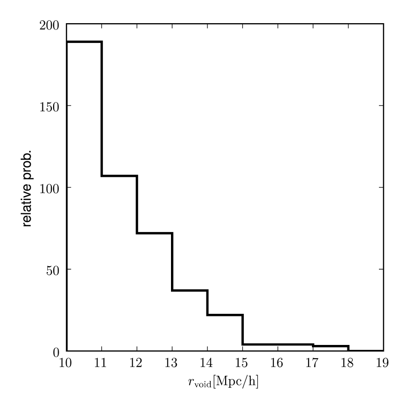
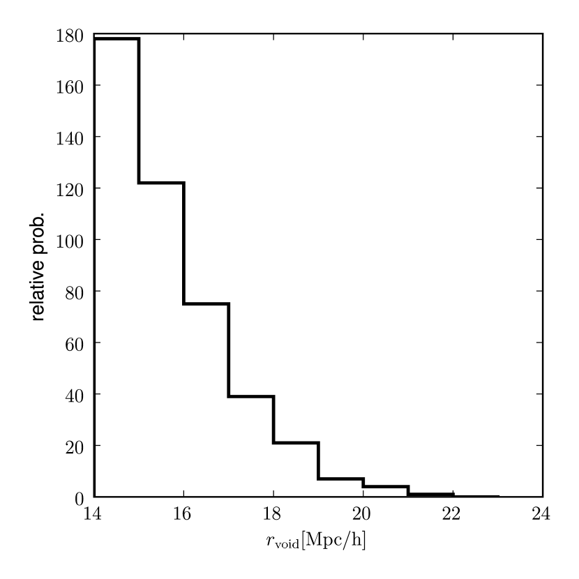
Figure 1: This figure shows the distribution of voids sizes for $m_{L}=-21$ (top) and $m_{L}=-22$ (bottom). Note that the minimum void size is an input parameter for the void finder and equals to 10 and 14 Mpc/$h$ respectively.

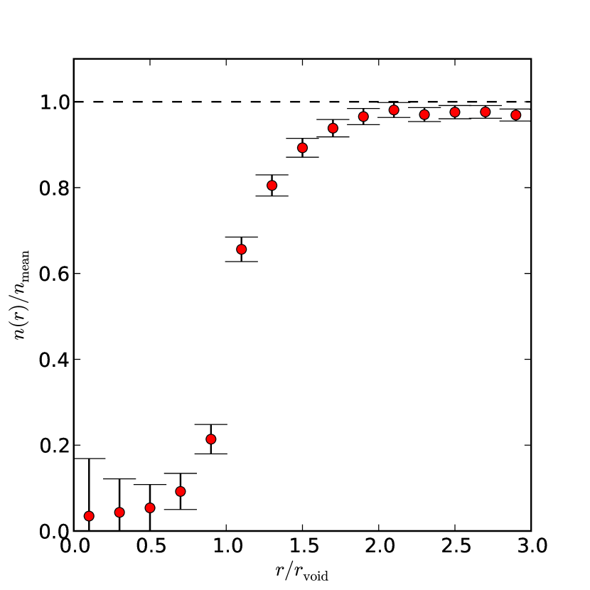
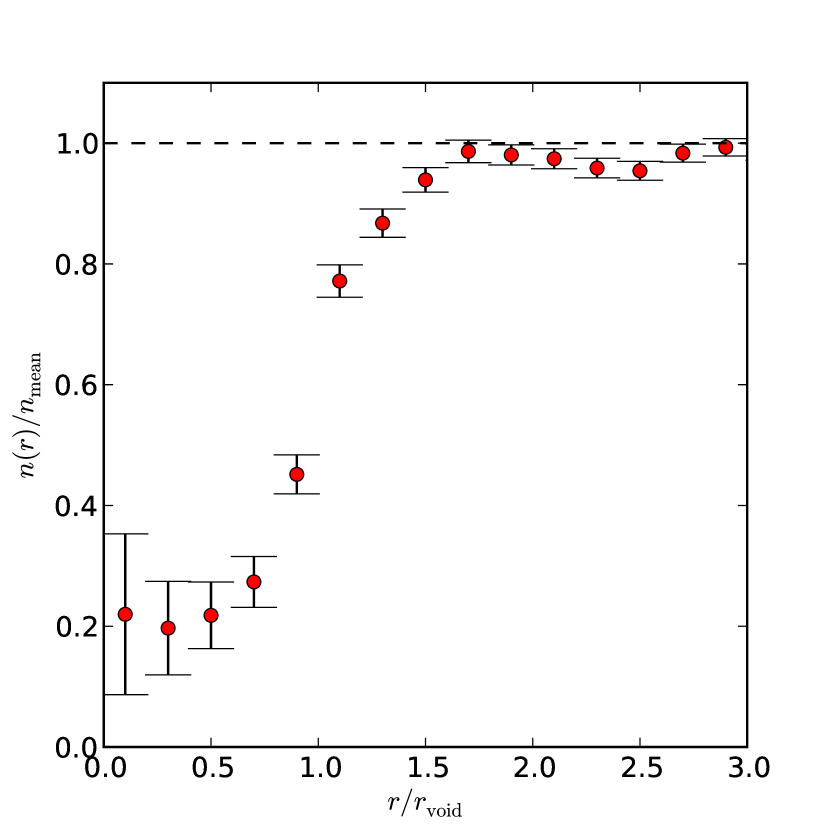
Figure 2: This figure shows how the mean number density of galaxies change as a function of distance from the void centre scaled by the void radius for the $m_{L}=-21$ (top) and $m_{L}=-22$ (bottom) samples. Error-bars are derived from Monte Carlo simulations in which void centres are randomly positioned within the volume limited catalogue and are approximate and heavily correlated.

III.1 Void Finder

The void finder is conceptually based on the HB void finder of Patiri et al. (2006). We start by creating a volume limited catalogue of galaxies. We create two volume limited catalogues, depending on the limiting absolute extinction-corrected $r$-band Petrosian magnitude, which we choose to be either $m_{L}=-22$ or $m_{L}=-21$. We use only parts of the survey where the survey completeness described by the SDSS parameter FGOTMAIN is above 0.82 and randomly remove galaxies to make the sample uniformly complete at this level. In addition we also use the VAGC’s random catalogues to create random catalogues with the same selection function as the main catalogues, but with about ten times as many points. We then find voids using the following algorithm.

1. Pick a random point in the survey volume. Locate four closest neighbours in the real catalogue. Determine the sphere that is defined by these four points.

2. Find if any other real galaxies are inside the sphere. If so, diminish the radius accordingly.

3. If the sphere’s radius is less than $10$ Mpc$/h$ for the $m_{L}=-21$ or $14$ Mpc$/h$ for the $m_{L}=-22$, discard it and go back to 1.

4. Count the number of random points inside the sphere and if this number is more than two sigma below the number expected given the number density of random points, discard it and go back to 1. Moreover, if the first moment of radial vectors of random points inside the void is inconsistent with random, discard them and go back to 1. This step essentially ensures that the void is fully within the survey.

5. Compare the void candidate to the existing voids. If it touches any of the existing voids, then discard the smaller of the two. Check if the new void touches any other voids and discard those as well. This ensures that two close small voids are merged into a bigger one if possible.

This process is repeated for all random points. Its result is a catalogue of non-overlapping spherical voids that contain no galaxies that are brighter than $m_{L}$ (though less bright galaxies can be in the voids). Although not strictly ensured by the algorithm, we find that the order in which random points are taken does not matter - the number of void solutions that are affected by this is less than 0.5%. Some basic properties about the voids the we find are tabulated in the Table 1.

		$m_{L}=-21$			$m_{L}=-22$
Number of voids		438			447
Minimum void radius		10 Mpc$/h$			14 Mpc/$h$
Maximum void radius		17.8 Mpc$/h$			21.4 Mpc/$h$
redshift range		0.169 – 0.183			0.111 – 0.123
	face-on	edge-on	both	face-on	edge-on	both
Number of galaxies	255	323	578	151	107	258
Naïve $\chi^{2}$	25.0	16.4	17.6	21.8	20.0	22.5
MC derived $\chi^{2}$	23.9	14.1	16.8	20.0	18.5	21.8
Constraints on $c$		$c<0.11(0.13)$			$c<0.16(0.19)$

Table 1: This table shows the basic properties of voids that we find in our data and the resulting $\chi^{2}$ values for null model. The null model has no degrees of freedom and there are 20 datapoints. The 95% limits correspond to $\chi^{2}$ of 9.6 – 34.2. The bottom section shows 95% (99.7%) limits on the $c$ parameter. See text for discussion.

To aid systematic checks we also form an ensemble of random void catalogues. In this catalogue we take the real number of voids and their radii and distribute them non-overlappingly, but otherwise randomly within the survey volume.

Throughout we ignore the distinction between real space and redshift space. Since our voids are relatively large and separated from high-density peaks, this should be a relatively safe approximation.

We plot basic properties of our voids in Figures 1 and 2. These are here to illustrate the properties of our voids in broad brushes and to show the dependence of voids on the void-finding algorithm properties. The main thrust of this paper is to analyze the properties of galaxy spins in the vicinity of voids; we will return to properties of voids in a forthcoming publication.

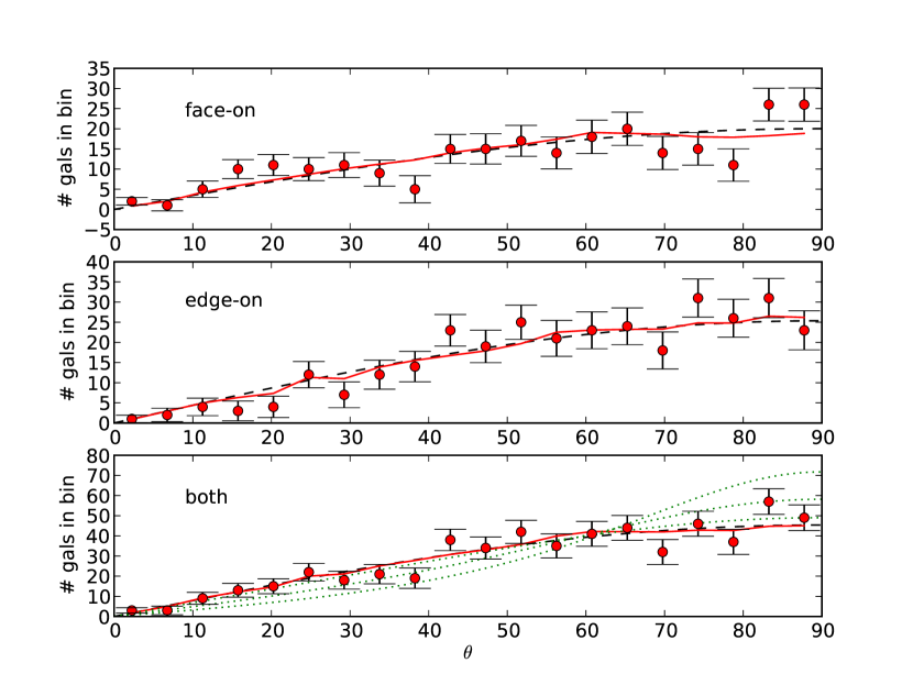
Figure 3: This figure shows the measured probability distribution for the angle $\theta$ in the $m_{L}=-21$ sample. Panels show results corresponding to face-on only (top), edge-on only (middle) and combined (bottom) spiral galaxies. The dashed black line corresponds to the theoretical expectation $p(\theta)=sin\theta$, while the solid red-line corresponds to the Monte Carlo results. The jaggedness in the red line is real and not a numerical artifact. Points are measurements with Monte Carlo derived errorbars. Dotted green lines are theoretical predictions for the models with $c=0.1,0.3,0.5$.

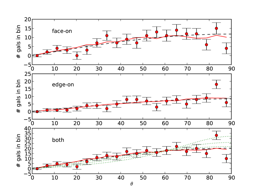
Figure 4: Same as Figure 3 but for a catalogue of voids derived from $m_{l}=-22$ volume limited sample.

III.2 Galaxies in the vicinity of voids

We next locate spiral galaxies that reside in the vicinity of voids. We now again work with the full SDSS catalogue and select spiral galaxies by a colour cut $g-r<0.6$, where $g$ and $r$ are model magnitudes from the SDSS pipeline. Spiral galaxy is considered to be at the edge of a void if its distance to the void centre is between $r_{\rm void}$ and $r_{\rm void}+r_{\rm taper}$, where $r_{\rm taper}=4{\rm Mpc}/h$ is the taper length. We limit ourselves to either face-on or edge-on galaxies. To determine the inclination of the galaxy, we use the adaptive moments $e_{+}$ and $e_{\times}$ from the SDSS photometric data reduction and calculate the axis ratio $q$ using Ryden (2004):

$$q=\left(\frac{1-e}{1+e}\right)^{1/2},$$ (10)

where $e=\sqrt{e_{\times}^{2}+e_{+}^{2}}$. Galaxies whose $q>0.96$ are deemed to be face on and those with $q<0.27$ are edge one. These criteria are somewhat more relaxed than those of Trujillo et al. (2006), but visual inspection of a random sub-sample ensured that we are indeed selecting face-on and edge-on spiral galaxies. For face-on galaxies, we assumed that the angular momentum axis is aligned with the radial direction toward the galaxy. Similarly, for the edge-on galaxies it was assumed to lie in the plane perpendicular to the radial direction and along the galaxies apparent minor axis. The latter was again inferred from the SDSS photometric reduction using the isophotal angle in the $r$-band and again visually confirmed to be measuring the correct quantity.

For the sample of galaxies and voids we then measure the probability distribution function for $\theta$, the angle between galaxy spin and the radial vector from the centre of the void toward the galaxy. Since the axis of the galaxy’s spin vector is a spin-2 quantity, the angle is constrained to lie between 0^∘ and 90^∘. We therefore measure the probability distribution function for this angle in 20 bins of uniform size in this range. The distribution of $\theta$ should follow $\sin\theta$ is our sampling of galaxies around voids would be random and if there were no edge effects associated with voids. However, in practice, while the voids were required to lie within the survey, the voids fattened by the taper radius might lie outside survey. Moreover, the cosmic web makes the sampling of positions non-uniform. In order to correct for these effects, we Monte-Carlo (MC) our errorbars as follows. For all galaxies that lie in the vicinity of void, including those that are neither face-on or edge-on, we randomly permute their spin vector properties and calculate the resulting $p(\theta)$ for an ensemble of permutations. The question we are therefore asking is: given the number of face-on, edge-on and remaining galaxies in the vicinity of voids, what is the probability that this distribution is not random? Using Monte-Carlo simulations we calculate the number of galaxies expected in each $\theta$ bin and the correlations between adjacent bins. Moreover, under assumption of Gaussianity, this allows us to calculate the exact $\chi^{2}$ by inverting the correlation matrix.

IV Results

Our main results are plotted in Figures 3 and 4. These figures show the expected signal in red solid line. This was derived using Monte Carlo simulations explained in the previous section. The jaggedness in the line is real and corresponds to the concrete distribution of cosmic web around the particular voids that we find. The plotted errorbars are also derived from the Monte Carlo Simulation.

It is clear already from the picture, that there is no strong evidence for departure from expected signal. We quantify this in Table 1. In this table we quote two different $\chi^{2}$ values. The naïve $\chi^{2}$ are calculated assuming that the number of galaxies in each bin is Poisson distributed and that bins are independent. The Monte-carlo derived $\chi^{2}$s use the mean values for null theory derived from the Monte Carlo simulations and evaluate $\chi^{2}$ taking in account the full covariance properties from MC samples. Since there are twenty data-points at which we estimate $p(\theta)$, we note that there are no detections at greater than $2$ sigma.

We note that the correctly calculated $\chi^{2}$ is in fact surprisingly close to the naïvely calculated one. In fact, this is due to the large number of voids that can be found using the DR6 dataset. If we artificially limit the number of voids, the difference can be much larger. For example, taking the first 50 voids of the $m_{L}=-22$ sample, the $\chi^{2}$ for face-on galaxies drops from $45.3$ using naïve $\chi^{2}$ to $17.9$ using MC $\chi^{2}$ with twenty degrees of freedom. This corresponds to a drop from over 3 sigma detection to less than 1 sigma. It is therefore crucial for the spinologist’s peace of mind that $\chi^{2}$s are calculated robustly.

Next we calculate limits on the parameter $c$, which are also shown in the Table 1. Two magnitude bins give very strong, but also very similar constraints on $c$.

IV.1 Systematics

It is possible that there is some crucial aspect of the analysis which is adversely affecting our results. We therefore compare the stability of our results with respect to the following tweaks to our data reduction and find no significant change in our results:

1. Including galaxies inside the void.

2. Considering just galaxies inside the void.

3. Changing the major to minor axes ratios required for face-on and edge-on criteria. In particular, we tested using the same $q$ ratios as Trujillo et al. (2006), namely $q>0.978$ for face-on and $q<0.208$ for edge-on.

4. Removing the color cut. This significantly increases our catalogue of galaxies, which becomes heavily contaminated by ellipticals.

V Discussion & Conclusion

In this paper we have reconsidered the alignment of galaxy spin axes in the vicinity of voids. We find no statistical departure from random for the orientation of galaxy spin axis in the vicinity of voids. Expressed in terms of the $c$ parameter, we find very stringent limit on $c<0.11\ (0.13)$ at 95% (99.7%) confidence limits. These limits assume a toy model with perfectly spherical voids and sharp edges. These are only approximately true in reality, but the numbers that we report should give an idea about the size of allowed values of $c$. Our limits are consistent with most $N$-body simulations, but there is some tension with the largest signal found by Cuesta et al. (2007), which is $c\sim 0.15$.

Our results are also inconsistent with previous results of Trujillo et al. (2006), who find $c=0.7^{+0.1}_{-0.2}$. The reasons for this discrepancy are not immediately clear, but we note that the catalogue that we use is considerably larger and has a much better filling factor that dramatically increases the number of voids. It possible that the results of Trujillo et al. (2006) were simply a statistical fluctuation.

When compared to the $N$-body simulations, the tidal torque theory seems to give qualitatively, but not quantitatively correct results (Porciani, Dekel, and Hoffman, 2002a, b). The ansatz of Equation (4) is perhaps less universally applicable. It was found to work reasonably well in early data Pen et al. (2000); however, there was recently a tentative detection of correlation of spin vectors that should vanish in this theory Slosar et al. (2008). In this paper we find $c$ is consistent with zero. Moreover, there does not seem to be good evidence for decoupling of scales between the tidal field and the local moment of inertia; a simplistic $k$-counting gives the same scale dependence. Finally, it is not clear whether the parameter $c$ should have one universal value or be an environment or scale-dependent variable.

On the basis of our revisiting the alignment of galaxy spins in the vicinity of voids we are again able to reconcile results from $N$-body simulations with observations. This is especially important in the light of the forth-coming weak lensing surveys; a nagging discrepancy between simulations and observations might lower our trust in corrections and systematic errors due to intrinsic alignment that are derived from $N$-body simulations. While more work must be done, the outlook is currently quite positive.

References

- Rees and Ostriker (1977) M. J. Rees and J. P. Ostriker, Mon. Not. R. Astron. Soc. 179, 541 (1977), ADS.
- Silk (1977) J. Silk, Astrophys. J. 211, 638 (1977), ADS.
- White and Rees (1978) S. D. M. White and M. J. Rees, Mon. Not. R. Astron. Soc. 183, 341 (1978), ADS.
- Fall and Efstathiou (1980) S. M. Fall and G. Efstathiou, Mon. Not. R. Astron. Soc. 193, 189 (1980), ADS.
- Blumenthal et al. (1984) G. R. Blumenthal, S. M. Faber, J. R. Primack, and M. J. Rees, Nature (London) 311, 517 (1984), ADS.
- Schneider (2006) P. Schneider, Weak Gravitational Lensing (Gravitational Lensing: Strong, Weak and Micro, Saas-Fee Advanced Courses, Volume 33. ISBN 978-3-540-30309-1. Springer-Verlag Berlin Heidelberg, 2006, p. 269, 2006), pp. 269–+.
- Hu (1999) W. Hu, Astrophys. J. Lett. 522, L21 (1999), ADS.
- Brown et al. (2002) M. L. Brown, A. N. Taylor, N. C. Hambly, and S. Dye, Mon. Not. R. Astron. Soc. 333, 501 (2002), ADS.
- Lee and Pen (2002) J. Lee and U.-L. Pen, Astrophys. J. Lett. 567, L111 (2002), ADS.
- Heymans et al. (2004) C. Heymans, M. Brown, A. Heavens, K. Meisenheimer, A. Taylor, and C. Wolf, Mon. Not. R. Astron. Soc. 347, 895 (2004), ADS.
- Mandelbaum et al. (2006) R. Mandelbaum, C. M. Hirata, T. Broderick, U. Seljak, and J. Brinkmann, Mon. Not. R. Astron. Soc. 370, 1008 (2006), arXiv:astro-ph/0507108.
- Faltenbacher et al. (2008) A. Faltenbacher, C. Li, S. D. M. White, Y. P. Jing, S. Mao, and J. Wang, ArXiv e-prints (2008), arXiv:0811.1995.
- Heymans et al. (2006) C. Heymans, M. J. White, A. Heavens, C. Vale, and L. Van Waerbeke, MNRAS 371, 750 (2006), arXiv:astro-ph/0604001.
- Hui and Zhang (2002) L. Hui and J. Zhang (2002), arXiv:astro-ph/0205512.
- Lee and Pen (2008) J. Lee and U.-L. Pen, Astrophys. J. 681, 798 (2008), arXiv:0707.1690.
- Sheth and van de Weygaert (2004) R. K. Sheth and R. van de Weygaert, Mon. Not. R. Astron. Soc. 350, 517 (2004), arXiv:astro-ph/0311260.
- van den Bosch et al. (2002) F. C. van den Bosch, T. Abel, R. A. C. Croft, L. Hernquist, and S. D. M. White, Astrophys. J. 576, 21 (2002), ADS.
- Bailin and Steinmetz (2005) J. Bailin and M. Steinmetz, Astrophys. J. 627, 647 (2005), arXiv:astro-ph/0408163.
- Patiri et al. (2006) S. G. Patiri, J. Betancort-Rijo, F. Prada, A. Klypin, and S. Gottlober, MNRAS 369, 335 (2006), arXiv:astro-ph/0506668.
- Brunino et al. (2007) R. Brunino, I. Trujillo, F. R. Pearce, and P. A. Thomas, MNRAS 375, 184 (2007), arXiv:astro-ph/0609629.
- Cuesta et al. (2007) A. J. Cuesta, F. Prada, A. Klypin, and M. Moles (2007), arXiv:0710.5520.
- Hahn et al. (2007) O. Hahn, C. M. Carollo, C. Porciani, and A. Dekel (2007), arXiv:0704.2595.
- Paz et al. (2008) D. Paz, F. Stasyszyn, and N. Padilla (2008), arXiv:0804.4477.
- Trujillo et al. (2006) I. Trujillo, C. Carretero, and S. G. Patiri, Astrophys. J. Lett. 640, L111 (2006), arXiv:astro-ph/0511680.
- Peebles (1969) P. J. E. Peebles, Astrophys. J. 155, 393 (1969), ADS.
- Doroshkevich (1970) A. G. Doroshkevich, Astrofizika 6, 581 (1970).
- White (1984) S. D. M. White, Astrophys. J. 286, 38 (1984), ADS.
- Heavens and Peacock (1988) A. Heavens and J. Peacock, Mon. Not. R. Astron. Soc. 232, 339 (1988), ADS.
- Catelan and Theuns (1996) P. Catelan and T. Theuns, Mon. Not. R. Astron. Soc. 282, 436 (1996), arXiv:astro-ph/9604077.
- Lee and Pen (2000) J. Lee and U. Pen, Astrophys. J. Lett. 532, L5 (2000), ADS.
- Lee (2004) J. Lee, Astrophys. J. Lett. 614, L1 (2004), arXiv:astro-ph/0408251.
- York et al. (2000) D. G. York et al., Astron. J. 120, 1579 (2000), ADS.
- Adelman-McCarthy et al. (2008) J. K. Adelman-McCarthy et al., Astrophys. J. Supp. 175, 297 (2008), arXiv:0707.3413.
- Blanton et al. (2005) M. R. Blanton, D. J. Schlegel, M. A. Strauss, J. Brinkmann, D. Finkbeiner, M. Fukugita, J. E. Gunn, D. W. Hogg, Ž. Ivezić, G. R. Knapp, et al., Astron. J. 129, 2562 (2005), arXiv:astro-ph/0410166.
- Ryden (2004) B. S. Ryden, Astrophys. J. 601, 214 (2004), arXiv:astro-ph/0310097.
- Porciani et al. (2002a) C. Porciani, A. Dekel, and Y. Hoffman, MNRAS 332, 325 (2002a), arXiv:astro-ph/0105123.
- Porciani et al. (2002b) C. Porciani, A. Dekel, and Y. Hoffman, MNRAS 332, 339 (2002b), arXiv:astro-ph/0105165.
- Pen et al. (2000) U. Pen, J. Lee, and U. Seljak, Astrophys. J. Lett. 543, L107 (2000), ADS.
- Slosar et al. (2008) A. Slosar, K. Land, S. Bamford, C. Lintott, D. Andreescu, P. Murray, R. Nichol, M. J. Raddick, K. Schawinski, A. Szalay, et al., ArXiv e-prints (2008), arXiv:0809.0717.