Classification of life by the mechanism of genome size evolution

Abstract

The classification of life should be based upon the fundamental mechanism in the evolution of life. We found that the global relationships among species should be circular phylogeny, which is quite different from the common sense based upon phylogenetic trees. The genealogical circles can be observed clearly according to the analysis of protein length distributions of contemporary species. Thus, we suggest that domains can be defined by distinguished phylogenetic circles, which are global and stable characteristics of living systems. The mechanism in genome size evolution has been clarified; hence main component questions on C-value enigma can be explained. According to the correlations and quasi-periodicity of protein length distributions, we can also classify life into three domains.

1 Background and motivation

In the absence of any ancient genetic sequences, scientists in the field of molecular evolution have to figure out reasonable mechanisms to retrieve the evolutionary history according to the genetic information of contemporary species. Traditionally, the basis for a natural taxonomy was provided by complex morphologies and a detailed fossil record. With the sequencing revolution, we had a new opportunity to understand the richer and more credible information on the evolution of life stored in the molecular sequences. Consequently, the basis for the definition of taxa has progressively shifted from the organismal to the cellular to the molecular level. Based upon rRNA sequence comparisons, life on this planet can be divided into three domains: the Bacteria, the Archaea, and the Eucarya [1]. The differences that separate the three domains are of a more profound nature than the differences that separate classical five kingdoms (Monera, Protista, Fungi, Plantae, Animalia).

The protein length evolution is poorly understood at present. The protein lengths vary notably both within a proteome and among species, and the average protein lengths of eukaryotes are longer than the average protein lengths of prokaryotes in general [2] [3]. But there are factors to increase or to decrease protein length, and it is still unclear whether in general protein tends to increase in length. [4] [5] [6]. Abound evidence indicates that there is underlying order in protein sequence organization. It is generally supposed that there are various structural and functional units in protein sequences. Periodicity was observed in protein length distributions [7] [8]. There is evidence for short-range correlation of protein lengths according to investigation by detrended fluctuation analysis [9] [10]. The correspondence between biology and linguistics at the level of sequence and lexical inventories, and of structure and syntax, has fuelled attempts to describe genome structure by the rules of formal linguistics [11] [12]. So Zipf’s law, originally found in linguistics, can be used to study the rank-size distribution of protein lengths [10] [12].

We found that protein length distributions can be taken as concise and comprehensive records of the evolution of life. The protein length should not be taken as a random quantity. The orders in protein lengths have been recorded in protein length distributions. We found profound relationship between the protein length evolution and genome size evolution. So we may unravel the mechanism of genome size evolution by the properties of protein length distributions. We found that the global taxonomy of life can be illustrated as phylogenetic circles rather than phylogenetic trees. Considering that phylogenetic circles are stable characteristics of living systems, we suggest that the circular phylogenetic relationship can be taken as a new criterion to identify domains.

The motivation of this work is to study the mechanisms in genome evolution based on properties of protein length distributions; consequently we can classify life in a global scenario of phylogenetic circles. We can explain (i) the trend of genome size evolution at the levels of domains and phyla, (ii) the patterns of genome size distributions, (iii) the bidirectional driving force in genome size evolution. At last, we successfully classify life into three domains based on properties of protein length distributions.

When trying to infer the early history of life according to the present biological data, we can borrow some smart ideas in physics. There is an analogy between the study of stellar evolution based on present experimental data of stellar spectra and the current task to infer the evolutionary history of life based on the protein length distributions. Although only the contemporary data can be observed in both cases, we can take the current states of stars, or of species, as various stages of their evolution. In the former case in astronomy, the Hertzsprung-Russell diagram shows a group of stars in various stages of their evolution according to the relation of absolute magnitude to stellar color, which is helpful to understand stellar evolution [13] [14]. In the latter case in the study of molecular evolution, some similar diagrams can also be plotted to show a group of species in various stages of their evolution based on protein length distributions.

2 Correlation analysis and spectral analysis of protein length distributions

Data collection. The data process in this paper is based on the biological data. In most calculations based on biological data in the paper, the protein length distributions are obtained from the data of $n=106$ complete proteomes ($n^{b}=85$ bacteria, $n^{a}=12$ archaea, $n^{e}=7$ eukaryotes and $n^{v}=2$ viruses) in the database Predictions for Entire Proteomes (PEP) [15]. Only in the cases when we study the detailed properties of genealogical circles and bifurcation of genome size distribution, the protein length distributions are obtained from both $n=106$ species in PEP and $775$ species in the National Center for Biotechnology Information (NCBI).

We denote $s(\alpha)$ as the genome size of species $\alpha$ and $\eta(\alpha)$ as the ratio of non-coding DNA to the total genetic DNA of species $\alpha$. The data of $\eta(\alpha)$ and $s(\alpha)$ are obtained from Ref. [16], where there are $54$ species ($6$ eukaryotes, $5$ archaebacteria and $43$ eubacteria) can be also found in PEP. The gene numbers $N$ are obtained by the numbers of Open Reading Frames (ORFs) in proteomes in PEP. There are $s(\alpha)\eta(\alpha)$ base pairs (bp) non-coding DNA and $s(\alpha)(1-\eta(\alpha))$ bp coding DNA in the genome of species $\alpha$.

Protein length distribution. We can definitely obtain the protein length distribution of a species if the lengths of proteins in its proteome are known. In calculation of a protein length distribution, we only concern the protein-coding genes and count only once for a gene with more than one copies. The transposable elements contribute little in calculation of protein length distributions. For instance, there are only dozens of genes appear to have been derived from transposable elements in human genome [17].

The protein length distribution of a species $\alpha$ can be denoted by a vector

$${\mathbf{x}(\alpha)}=(x_{1}(\alpha),x_{2}(\alpha),...,x_{k}(\alpha),...),$$ (1)

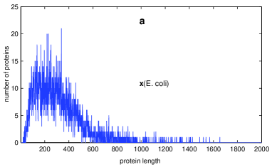
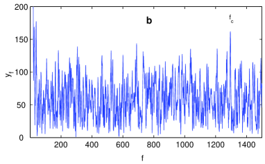
Figure 1: Protein length distribution and power spectrum of E. coli. a, Protein length distribution ${\mathbf{x}}$(E. coli). b, The power spectrum ${\mathbf{y}}$(E. coli), the characteristic frequency $f_{c}$ at the highest peak is marked.

where there are $x_{k}(\alpha)$ proteins, whose lengths are just $k$ amino acids (a.a.), in the entire proteome of this species (Fig. 1a). The average protein length in the proteome of species $\alpha$ can be calculated by the protein length distribution:

$$\bar{l}(\alpha)=\frac{\sum_{k=1}^{m}k\ x_{k}(\alpha)}{\sum_{k=1}^{m}x_{k}(\alpha)}.$$ (2)

And the standard deviation of protein lengths can be calculated by:

$$\Delta l(\alpha)=\sqrt{\frac{\Sigma_{k=1}^{m}x_{k}(\alpha)(k-\bar{l}(\alpha))^{2}}{\Sigma_{k=1}^{m}x_{k}(\alpha)}}$$ (3)

The total protein length distribution of all the species in PEP is denoted by

$$\mathbf{X}=\sum_{\alpha\in\mbox{\tiny PEP}}\mathbf{x}(\alpha).$$ (4)

Since there are few quite long proteins, it is practical to choose a sufficient large protein length as the cutoff of protein length in the protein length distributions in the data process. Here, we set the cutoff as $m=3000$ amino acids (a.a.). Almost all the neglected elements of protein length distributions, i.e., $x_{i}(\alpha),\ i>m$, vanish according to the biological data in PEP, which contribute little in our data analysis. So our conclusions are free from the choice of $m$.

A peak in the fluctuations of protein length distribution $\mathbf{x}(\alpha)$ can be distinguished when $x_{l}(\alpha)$ is greater than both $x_{l-1}(\alpha)$ and $x_{l+1}(\alpha)$. The number of peaks of protein length distribution $\mathbf{x}(\alpha)$ can be denoted by $p(\alpha)$. There is no smoothing for protein length distributions when counting the number of peaks. So $p(\alpha)$ can be obtained rigorously for any species whose proteome is know. There is profound biological meaning for peak number $p$.

Correlation analysis. Given any pair of species $\alpha$ and $\beta$ in PEP, we will find several ways to evaluate the correlation between the protein length distributions of any pair of species. Accordingly, we can calculate the corresponding average correlation between any species and all the species in PEP. The correlation polar angle $\theta(\alpha)$ of species $\alpha$ is defined as the angle between vectors $\mathbf{x}(\alpha)$ and $\mathbf{X}$, i.e.

$$\theta\equiv\frac{2}{\pi}\arccos(\frac{{\mathbf{x}}\cdot{\mathbf{X}}}{\left|\left|{\mathbf{x}}\right|\right|\left|\left|{\mathbf{X}}\right|\right|}),$$ (5)

where the factor $\frac{2}{\pi}$ is added in order that the value of $\theta$ ranges from $0$ to $1$. The less the value of $\theta(\alpha)$ is, the closer the average correlation of protein length distribution for species $\alpha$ is.

The correlation coefficient of protein length distributions between species $\alpha$ and $\beta$ is defined by

$$r(\alpha,\beta)=\frac{\sum_{k=1}^{m}(x_{k}(\alpha)-\bar{x}({\alpha}))(x_{k}(\beta)-\bar{x}({\beta}))}{\sqrt{\sum_{k=1}^{m}(x_{k}(\alpha)-\bar{x}({\alpha}))^{2}}\sqrt{\sum_{k=1}^{m}(x_{k}(\beta)-\bar{x}({\beta}))^{2}}},$$ (6)

where $\bar{x}({\alpha})=\frac{1}{m}\sum_{k=1}^{m}x_{k}(\alpha)$. And the average correlation coefficient of species $\alpha$ can be defined by

$$R(\alpha)=\frac{1}{106}\sum_{\beta\in\mbox{\tiny PEP}}r(\alpha,\beta).$$ (7)

The value of $R(\alpha)$ ranges from $0$ to $1$. The more the value of $R$ is, the closer the average correlation of protein length distributions is.

The Minkowski distance between species $\alpha$ and $\beta$ is defined by

$$d(\alpha,\beta)=(\sum_{k=1}^{m}\left|\frac{x_{k}(\alpha)}{\left|\left|\mathbf{x}(\alpha)\right|\right|}-\frac{x_{k}(\beta)}{\left|\left|\mathbf{x}(\beta)\right|\right|}\right|^{q})^{1/q},$$ (8)

where $q$ is a parameter. And the average Minkowski distance of species $\alpha$ can be defined by

$$D(\alpha)=\frac{1}{106}\sum_{\beta\in\mbox{\tiny PEP}}d(\alpha,\beta).$$ (9)

The less the value of $D$ is, the closer the average correlation of protein length distributions is.

Spectral analysis. We can study the order in the fluctuations in the protein length distributions by the method of spectral analysis. The discrete fourier transformation of the protein length distribution $\mathbf{x}(\alpha)$ is:

$$\hat{x}_{f}(\alpha)=\frac{1}{\sqrt{m}}\sum_{k=1}^{m}x_{k}(\alpha)e^{2\pi i(k-1)(f-1)/m}.$$ (10)

The power spectrum, i.e., the abstract of the discrete fourier transformation, is defined as (Fig. 1b)

$${\mathbf{y}(\alpha)}=\left|\left|\hat{\mathbf{x}}(\alpha)\right|\right|=\sqrt{(\mbox{Re}\ \hat{\mathbf{x}}(\alpha))^{2}+(\mbox{Im}\ \hat{\mathbf{x}}(\alpha))^{2}}.$$ (11)

The power spectrum $\mathbf{y}=(y_{1},...,y_{m})$ is mirror symmetric between $(y_{1},...,y_{m/2})$ and $(y_{m/2+1},...,y_{m})$ according to the properties of discrete Fourier transformation.

The peaks in the power spectrum $\mathbf{y}(\alpha)$ relate to the periodicity of fluctuations in the protein length distribution $\mathbf{x}(\alpha)$. In the following, we only considered the left half of the power spectrum $(y_{1},...,y_{m/2})$, while the properties on the right half are alike by mirror symmetry. Besides, we neglected the power spectrum at very low frequency where the peaks are always high due to the general bell-shape profiles of protein length distributions. The high frequency sector refers to the power spectrum at $f$ near to $m/2$, and the low frequency sector refers to the power spectrum at $f$ much less than $m/2$. The characteristic frequency of the highest peak in the left half of the power spectrum $(y_{1}(\alpha),...,y_{m/2}(\alpha))$ can be denoted by $f_{c}(\alpha)$ (Fig. 1b). Moreover, we can find the top $n_{p}$ highest peaks in the fluctuations of the left half of the power spectrum. The maximum frequency of the frequencies for the above top $n_{p}$ highest peaks can be denoted by $f_{m}(\alpha)$, whose original intention is to determine an obvious peak with large frequency. 7a - 7c). And we defined the characteristic period $L_{c}$ and minimum period $L_{m}$ of the fluctuations of protein length distribution as follows:

$$L_{c}(\alpha)=m/f_{c}$$ (12)

$$L_{m}(\alpha)=m/f_{m},$$ (13)

which are free of the choice of the cutoff $m$. We chose $n_{t}=30$ for $f_{m}^{\prime}$ and $L_{m}^{\prime}$ and $n_{t}=80$ for $f_{m}^{\prime\prime}$ and $L_{m}^{\prime\prime}$ in the calculation.

The average power spectra for three domains (Bacteria, Archaea and Eucarya) are as follows respectively:

$$\mathbf{y}^{b}=\frac{1}{n^{b}}\sum_{\alpha\in\mbox{\tiny Bacteria}}\mathbf{y}(\alpha)$$ (14)

$$\mathbf{y}^{a}=\frac{1}{n^{a}}\sum_{\alpha\in\mbox{\tiny Archaea}}\mathbf{y}(\alpha)$$ (15)

$$\mathbf{y}^{e}=\frac{1}{n^{e}}\sum_{\alpha\in\mbox{\tiny Eucarya}}\mathbf{y}(\alpha).$$ (16)

3 Calculation of genome size and non-coding DNA content

Calculation of genome size. The genome size evolution is one of the central problems in the study of molecular evolution because it is a macroevolutionary question and is helpful to understand the large-scale patterns in the history of life [18][19]. We had found a close relationship between genome size $s$ and the correlation $\theta$ of protein length distributions and non-coding DNA content $\eta$ in a previous work [20], hence the genome size of contemporary species can be calculated by an experimental formula with two variants. In this paper, we also found a close relationship between genome size $s$ and the peak number $p$, then we obtained another single-variant experimental formula to calculate the genome sizes. According to the relationship between the two formulae, we can obtain an experimental formula to calculate the non-coding DNA content $\eta$ only based on the data of coding DNA. This interesting result infers that the non-coding DNA content depends on the coding DNA.

In the previous work, we found that the genome size $s$ relates to two variants: the non-coding DNA content $\eta$ and the correlation polar angle $\theta$. Hence we had obtained a double-variant experimental formula to calculate the genome size of a certain species [20]

$$s(\eta,\theta)=s_{0}\exp(\frac{\eta}{a}-\frac{\theta}{b}),$$ (17)

where $s_{0}=7.96\times 10^{6}$ bp, $a=0.165$ and $b=0.176$. The crux to obtain this formula is to find the proportional relationship between genome size $s$ and correlation polar angle $\theta$ for prokaryotes. The biological meaning of $\theta(\alpha)$ is the average correlation of protein length distributions between species $\alpha$ and all the other species. Furthermore, we naturally introduced the second variant $\eta$ in the formula so that this formula can be generalized for eukaryotes. For the prokaryotes, the non-coding DNA contents are about $10$ percent, but the correlation polar angles range from about $0.6$ to $0.1$. For the eukaryotes, the correlation polar angles are around $0.1$, but the non-coding DNA contents range from $0.1$ to near $1$. This double-variant formula is well-predicted not only for prokaryotes but also for eukaryotes. We also proposed a formula to describe the trend of genome size evolution [20]

$$s(t)=s_{0}\exp(\frac{\eta(t)}{a}-\frac{\theta(t)}{b}).$$ (18)

Thus the dynamic parameter $\eta(t)$ and $\theta(t)$ become promoting factor and hindering factor in determining the trend of genome size evolution.

In this paper, we found another single-variant experimental formula to calculate the genome size. We found that there is an exponential relationship between genome size $s$ and number of peaks $p$:

$$s(p)=s^{\prime}\exp(\frac{p}{p_{0}}),$$ (19)

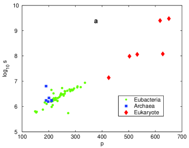
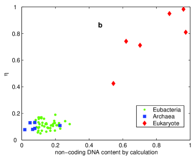
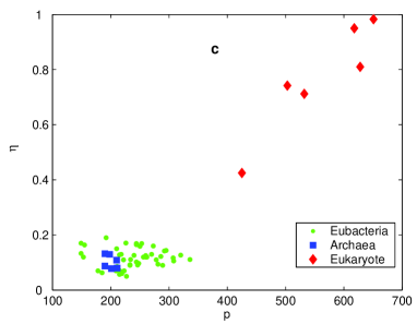
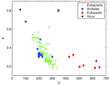
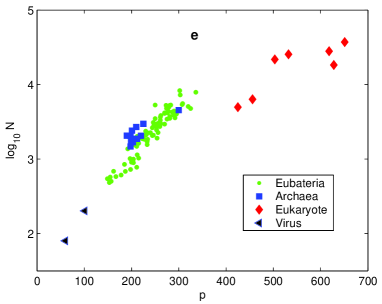
Figure 2: Prediction of genome size and non-coding DNA content. a, $p$ is proportional to $\log_{10}s$ (Correlation coefficient is $0.9428$). b, The non-coding DNA predicted by the formula agrees with the biological data (Correlation coefficient is $0.9468$). c, The relation between $p$ and $\eta$. d, The relation between $p$ and $\theta$. e, The relation between $p$ and $\log_{10}N$ is not linear (Correlation coefficient is $0.8747$).

where $s^{\prime}=8.36\times 10^{4}$ bp and $p_{0}=70.6$ are determined by least squares. There is only one variant $p$ in this formula. The prediction of genome sizes by this formula agrees with the biological data of genome sizes very well (Fig. 2a). The single-variant formula is also valid not only for prokaryotes but also for eukaryotes. Therefore, the genome sizes for both prokaryotes and eukaryotes can be investigated in a unified framework.

Calculate of non-coding DNA content. In terms of the relationship between the above two experimental formulae, we obtained an experimental formula to calculate the non-coding DNA content:

$$\eta(\alpha)=0.938\ \theta(\alpha)+0.00234\ p(\alpha)-0.752,$$ (20)

where both $\theta$ and $p$ are defined only based upon the protein length distributions. The prediction of the non-coding DNA contents agrees with the experimental observations (Fig. 2b). According to the formulae to calculate $s$ and $\eta$, we can calculate the size of coding DNA $(1-\eta)s$ as well as the size of non-coding DNA $\eta s$ according to the value of $p$ and $\theta$ for any species. At first thought, such a result is quite surprising. We can obtain the size of coding DNA directly from the protein length distribution: $(1-\eta)s=\Sigma_{i=1}^{m}ix_{i}$. There should be no direct evidence about the size of non-coding DNA according to the protein lengths in the coding DNA segment.

This result is profound because it shows that there is a close relationship in sizes between non-coding DNA segment $\eta s$ and coding DNA segment $(1-\eta)s$. The evolution of non-coding DNA relates to the evolution of coding DNA, whose functions may relate closely to the cellular differentiation. The size of non-coding DNA can not be arbitrary if the protein length distribution $\mathbf{x}$ is given. The information about coding DNA is stored in the components $x_{i}$ of protein length distribution $\mathbf{x}$, where the order of components is irrelative to the result of calculation. The order of these component $x_{i}$, i.e., the order of fluctuations of protein length distribution $\mathbf{x}$ becomes significant for calculating the size of non-coding DNA. So there is additional evolutionary information stored in the fluctuations of protein length distributions.

The variant $p$ can be obtained directly from the protein length distribution of the species’ own, but the other variant $\theta$ depends on the data of protein length distributions of other species. The crux to define $\theta$ is to calculate the correlation of fluctuations of protein length distributions $\mathbf{x}$ and $\mathbf{X}$. It indicates that there is a universal mechanism for the genome size evolution for all the species. So the variant $\theta$, as an average value of correlation, is essential in calculation of non-coding DNA content.

Relationship between $p$ and $\eta$, $\theta$. Genome size evolution provides a clear example of hierarchy in action. No one-dimensional explanation can account for the massive variation in eukaryotic genome sizes [19]. The success of the double-variant formula to calculate the genome size benefits from the proper choice of two variants $\theta$ and $\eta$. But why can we also find a formula to calculate genome size with only one variant $p$? The correlation between genome size $s$ and peak number $p$ can not be explained trivially by the observation that genome size and proteome size are correlated. The linear relationship between $p$ and $\log_{10}s$ shows that $p$ is an intrinsic genomic property of a species. The relationship between $p$ and $\log_{10}N$ is non-linear (Fig. 2e). The fluctuations of protein length distributions can no longer be taken as random fluctuations on the smooth background, which reflects the complexity of proteome and relates to the complexity of life.

We can understand the biological meaning of peak number according to the relationship between the single variant $p$ and the pair of variants $\eta$ and $\theta$. Firstly, we studied the relationship between $p$ and $\eta$ based on the biological data (see the distribution of species in Fig. 2c). We found that there is a critical value $p_{c}$ of peak number, which definitely separates prokaryotes and eukaryotes in the $p-\eta$ plane. For prokaryotes, $p$ is less than $p_{c}$ and $\eta$ is about constant. The distribution of species in the $\eta-p$ plane ($p<p_{c}$) consists a rightward triangle, which agrees with another triangle distribution of prokaryotes in $s-\eta$ plane (Fig. 3f) due to the correlation between peak number $p$ and genome size $s$. The deviation of $\eta$ from average value $0.1$ becomes smaller and smaller when $p$ goes to $p_{c}$. For eukaryotes, $p$ is greater than $p_{c}$ and $\eta$ increases with $p$. The distribution of species in the $\eta-p$ plane ($p>p_{c}$) consists a leftward triangle. The deviation of $\eta$ becomes bigger an bigger when $p$ goes away from $p_{c}$. So there are few species in the area $p\sim p_{c}$. Such a regular distribution of species in the $p-\eta$ plane indicates a profound relationship between $p$ and $\eta$. So $p$ can not be meaningless in biology. Secondly, we studied the relationship between $p$ and $\theta$ (Fig. 2d). We found that $\theta$ declines with $p$ for prokaryotes when $p<p_{c}$, while $\theta$ is about constant for eukaryotes when $p>p_{c}$. We point out that $p$ relates closely to the complexity of life. It was suggested that the non-coding DNA content $\eta$ indicates the complexity of eukaryotes: the larger the value of $\eta$ (corresponding to larger $p$) is, the more the complexity of eukaryotes is [21]. In the case of prokaryotes, the genome sizes, which are proportional to the gene numbers, can indicate the complexity of prokaryotes because the non-coding DNA contents are about the same for prokaryotes. Thus, the larger genome size (corresponding to larger $p$) is, the more complexity of prokaryotes is. A natural meaning of peak number $p$ is an index for the complexity of structures of any protein length distribution. Summarizing the above, we suggest that peak number $p$ indicates the meaning of complexity of life.

In order to understand peak number $p$ more clearly, we deduced its evolutionary formula according to the formula on the evolutionary trend of genome size in Ref. [20]:

$$s(t)=\left\{\begin{array}[]{rr}s_{1}\exp t/\tau_{1},&t<T_{c}\\ s_{2}\exp t/\tau_{2},&t>T_{c}\end{array}\right.,$$ (21)

where $T_{c}=-560$ Million years (Myr) ($t=0$ for today) and $\tau_{1}=644$ Myr, $\tau_{2}=106$ Myr, $s_{1}=1.98\times 10^{7}$ bp and $s_{2}=1.65\times 10^{9}$ bp. We obtained that there were two stages in the evolution of peak number:

$$p(t)=\left\{\begin{array}[]{rrr}\frac{p_{0}}{\tau_{1}}t+p_{0}\ln\frac{s_{1}}{s^{\prime}}=0.110t+386,&t<T_{c}\\ \frac{p_{0}}{\tau_{2}}t+p_{0}\ln\frac{s_{2}}{s^{\prime}}=0.666t+698,&t>T_{c}\end{array}\right..$$ (22)

The critical peak number in the evolution is $p_{c}=p(T_{c})=p_{0}\ln\frac{s_{0}}{s^{\prime}}=324$. We found that peak number evolves much faster in the period after $T_{c}$ than in the period before $T_{c}$. Since peak number did not evolve evenly, it can not be regarded as an independent variant in the evolution. The variant $p$ is underlain by two variants $\eta$ and $\theta$. So the genome size always needs two-dimensional explanation.

4 Phylogenetic circles in $\Delta l-p$ plane and bifurcation of genome size distribution in $\Delta l-s$ plane

Phylogenetic circles in $\Delta l-p$ plane. Previously, we have explained several main problems in C-value enigma, such as the genome ranges in taxa and genome size distribution, according to the two-variant genome size formula [20] [18]. The biological meaning of this formula can be understood more clearly when we wrote down its derivative form as follows

$$\frac{\Delta s}{s}=\frac{\Delta\eta}{a}-\frac{\Delta\theta}{b}.$$ (23)

Evidently, there are two factors in control of the genome size evolution. The first variant $\eta$ is promoter, whose contribution is measured by $a$, and the other variant $\theta$ is hinderer, whose contribution is measured by $b$. The genome size evolution is a bidirectional course, which may either increase or decrease in the evolution.

We found a miraculous distribution of species in $\Delta l-p$ plane (Fig. 3a). The eukaryotes, archaea and eubacteria distribute in three circular areas respectively. The species distribute only on the edges of the circles, and it is empty within the circles. It is obvious to form a circle by several samples of eukarya, archaea and mycoplasma respectively. Even for eubacteria, we can also observe a distribution with an empty center enclosed by a round boundary. The two virus are also near to each other. We can conclude that there is almost no exception of species that disassociate these observed circles.

The standard deviation of protein length $\Delta l$ and the peak number in protein length distribution $p$ are pivotal properties in studying genome size evolution. $\Delta l$ relates to the variation of protein length by its definition. And we can consider $p\sim\frac{\eta}{a}-\frac{\theta}{b}$ as the “net driving force” in genome size evolution.

Global patterns of genomes size variation at the levels of domains and phyla. In order to observe the phylogenetic circles in more detail, we obtained more protein length distributions based on the biological data of $775$ microbes ($725$ eubacteria, $50$ archaea) in NCBI. The microbial taxonomy in this work is based on the NCBI taxonomy database [22] [23]. Thus, we can obtain a detailed distribution of microbes in $\Delta l-p$ plane. At the level of domains, we can also observe two phylogenetic circles for eubacteria and archaea respectively (Fig. 4a).

Too many proteobacteria (blue legends in Fig. 4a) in the database disturbed us to discern the phylogenetic circle of eubacteria easily. So we divide the $725$ eubacteria into two groups: “the group of $397$ proteobacteria” and “the group of the other $328$ eubateria”. Thus, we can discern the phylogenetic circle of eubacteria. For the group of “the other $328$ eubateria”, we can observe a circular chain composed of $10$ phyla (Firmicutes, Acidobacteria, Actinobacteria, Cyanobacteria, Bacteroidetes/Chlorobi, Spirochaetes, Chlamydiae/Verrucomicrobia, Chloroflexi, Deinococcus-Thermus, Thermotogae) (Fig. 4b). This circular chain shows that the global picture of the distribution of eubateria are indeed a phylogenetic circle, although the numbers of species vary greatly among these $10$ phyla in the database. For the group of proteobacteria, the species from the five classes (Alphaproteobacteria, Betaproteobacteria, Gammaproteobacteria, Deltaproteobacteria and Epsilonproteobacteria) also form an arch of the phylogenetic circle at the same place of the circular chain of the other $10$ phyla (Fig. 4c). Especially, the species in the class of Alphaproteobacteria almost form a closed circular distribution.

According to the detailed observation of phylogenetic circle, we conjecture that the distribution of species in a same domain form a closed circle in $\Delta l-s$ plane, while the species in a phylum or lower taxon only form an arch of the circle. Namely, the global pattern of genomes size variation at the level of domains can be described by phylogenetic circles, while the pattern of genomes size variation at the levels of phyla and lower taxa only reflects local properties of the corresponding phylogenetic circle.

Bifurcation of genome size distribution in $\Delta l-s$ plane. The distribution of species in $\Delta l-s$ plane is very interesting, whose shape likes two wings of a butterfly (Fig. 3b). Considering the close relationship between $p$ and $s$, this distribution is similar to the one in $\Delta l-p$ plane. We can obviously observe two asymptotes that depart the plane into four quadrants. The origin $O$, i.e. the point of intersection of the asymptotes, corresponds to a special genome size $s^{*}$ (Fig. 3b). There is almost no species in the upper and lower quadrants. All bacteria gather either in left quadrant or right quadrant; archaea gather also in left or right quadrants, but only in the lower parts; all eukaryotes gather in the right quadrant, but in the upper part and far away from $s^{*}$; and the two virus gather in the left quadrant, but in the upper part and far away from $s^{*}$. The distribution of species in $\Delta l-N$ plane is also similar to the one in $\Delta l-p$ plane, but the circular shapes become worse (Fig. 3h).

We also obtained a more detailed distribution in $\Delta l-s$ plane based on the biological data of the $775$ microbes in NCBI. The overall shape of the distribution also likes a butterfly (Fig. 4d). Especially, the distribution of proteobacteria in $\Delta l-s$ plane agrees with a butterfly shape very well (Fig. 4e). We observed that the distribution of species in groups Alphaproteobacteria, Betaproteobacteria, Gammaproteobacteria also agree with the butterfly shape; while the species in groups Deltaproteobacteria and Epsilonproteobacteria distribute on the right wing and left wing respectively.

Though the distributions of archaea and eukaryotes obviously deviate the distribution of eubacteria, the overall distribution of all species does not violate the butterfly shape. The places of Archaea, Eubateria and Eukarya indicate that, at the level of domain, the greater the standard error of the protein length in a proteome is, the greater the genome size is.

The butterfly shaped distribution of species in $\Delta l-s$ plane is helpful for us to understand the variation of genome sizes, which strongly indicates the bidirectionality in genome size evolution. The genome size corresponding to the connection point of the two wings in Fig. 4d is approximately the same as the genome size corresponding to the center of phylogenetic circle in Fig. 4b. In the evolution of genome size for the closely related species, the genome size may either increase or decrease. It can be indicated that the increasing trend is considerably stronger than the decreasing trend in genome size evolution, because there are obviously more species on the right wing than on the left wing in the distribution of species in $\Delta l-s$ plane (Fig. 4d and 4e).

5 Unravelling the mechanism of genome size evolution

Global and local pictures of genome size evolution. A distinguished phylogenetic circle can be taken as a natural definition of a domain. The mechanism for the origin of domains is quite different from the mechanism for the origin of phyla. There are two significant events in the evolution of life: the origin of domains in early stage of evolution and the origin of animal phyla around Cambrian period [20] [24]. The phylogenetic circles only exist at the level of domain according to the distribution of species in $\Delta l-p$ plane. The properties at the level of domains do not couple with the later evolution at the levels of phyla and so forth. So phylogenetic circles are stable characteristics and may exist from the early stage in the evolution of life to present days. The observation of phylogenetic circles can be explained by Woese’s theory on cellular evolution [25]. According to his perspective, horizontal gene transfer is the principal driving force in early cellular evolution. The primitive cellular evolution is basically communal, and it is not the individual species that evolve at all. So genome cluster evolution is more essential than the evolution of an individual genome; and the study of the origin of a living system is much more valuable than the study of origin of just one species.

The phylogenetic circles are “global” properties, while the traditional conception of the phylogenetic trees is “local”. Although the phylogenetic tree is useful in many circumstances, it has unfortunately misled us to comprehend the panorama of taxonomy of life. In the global scenario, we emphasize the phylogenetic circle should evolve as a whole, while in the local scenario, a species can evolve freely along continually branching phylogenetic tree. The underlying mechanism on evolution must be a “global” theory. An individual life can never originate and evolve unless it existed as a phylogenetic circle of primordial life. A new theory of evolution of life is necessary to understand the evolution of a cluster of genomes as a whole. Then we may explain the trajectory of the phylogenetic circles in the $\Delta l-p$ plane in the evolution. The local properties of a phylogenetic circle is the same as the properties of phylogenetic tree, but we can not be aware of the global constraint in the local scenario.

Dynamics of genome size evolution. Due to the definite different topological properties between a circle and a tree, a mechanism of genome size evolution on a circle will quite differ from the traditional mechanisms of genome size evolution based on phylogenetic trees. The genome size can not increase unlimitedly when evolving in a circular pathway, but it can go to infinity in an unlimitedly branching pathway. So there is intrinsic mechanism to reduce the genome size which closely relates to the protein evolution. According to Eqn. (19) and Eqn. (20), we can calculate the genome size and the non-coding DNA size by $p$ and $\theta$, both of which are based on the data of protein length distributions. These experimental formulae indicate that protein evolution principally drives the genome size evolution.

The driving force in genome size evolution is bidirectional. Large scale gene duplications and accumulation of transposable elements are primary contributors in genome expansion. Whereas the reverse mechanism to reduce genome size was less understood. According to our scenario of phylogenetic circles, the global circular relationship in a domain must constrain the genome expansion. More explicitly speaking, genome size of a species has to evolve in the community of the domain; it can not evolve independently. In our previous work on the trend of genome size evolution, there are two dynamic factors (promotor $\eta$ and hinderer $\theta$) in determining the genome size evolution, where $\eta$ corresponds to the process of polyploidy and accumulation of transportable elements and $\theta$ indicates the relationships among species. So the biological meaning of the formula on genome size evolution just agrees with the explanation based on the scenario of phylogenetic circles.

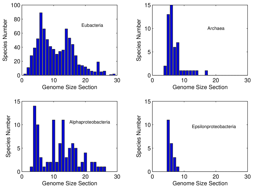
Figure 5: Genome size distributions. The width of each genome size section is $3.5\times 10^{6}$ bp.

Explanation of genome size distribution. According to the bifurcation of genome size distribution in $\Delta l-s$ plane, it is easy to explain the patterns of genome size distributions among taxa. There are two main types of genome size distributions: single-peak type and double-peak type. For single-peak type, the species in a certain taxon distribute on only one side of wing of the butterfly shaped distribution in $\Delta l-s$ plane, so the outline of the genome size distribution among this taxon has only one main peak. For double-peak type, the species in a certain taxon distribute on both wings of the butterfly shaped distribution in $\Delta l-s$ plane, so the outline of the genome size distribution among this taxon has two main peaks. For examples, the genome size distributions for Eukaryotes or for Alphaproteobacteria belong to double-peak type, and the genome size distributions for Archaea or for Epsilonproteobacteria belong to single-peak type (Fig. 5). The genome size distributions for eukaryotic taxa belong to single-peak type [18] [26], because eukaryotes all distribute on the right wing of the butterfly shaped distribution in $\Delta l-s$ plane.

On plant genome size evolution. Recent studies have made significant advances in understanding the mechanism of plant genome size evolution, where polyploidy and the accumulation of transposable element plays significant roles in plant genome expansion, although less is known about the process for DNA removal [26] [27] [28] [29] [30]. It is reported that “different land plant groups are characterized by different C-value profiles, distribution of C-values and ancestral C-values” [26]. In the viewpoint of phylogenetic circles, different land plant groups should situate on the Eukaryotic phylogenetic circle and form a circular chain that is similar to the bacterial circular chain in Fig. 4b. So it is natural to draw the above conclusion, because (i) ancestral C-values should spread around on the circular chain and (ii) the “local” properties on genome size evolution at different places on the phylogenetic circle should also differ among different plant groups.

The formulae on the trend of genome size evolution can explain the coding DNA and non-coding DNA interactions in genome evolution. Entire genome duplication contributes the majority of genome size increase in plants. Simple chromosome duplication may double the genome size on the left hand of Eqn. (17) or (19). However, the values of $\eta$ and $\theta$ or $p$ on the right hand of Eqn. (17) or (19) keep invariant because the protein length distribution does not change in simple chromosome duplication. The apparent contradiction to the trend of genome size evolution will urge the alternation of coding DNA so that $\eta$ and $p$ tend to increase in after the chromosome duplication. Such evolutionary pressure agrees with the experimental observations. After duplication, the two copies of the gene are redundant. Because one of the copies is freed from functional constraint, mutations in this gene will be selectively neutral and will most often turn the gene into a nonfunctional pseudogene [18]. Hence, the ratio of non-coding DNA $\eta$ will increase. On the other hand, gene duplication can provide source of material for the origin of new genes with to alternative length [28]. Consequently, the protein length distribution will change to be more complex and the peak number $p$ will be urged to increase. So $p$ intrinsically measures the protein evolution. Due to the rapid adjustment shortly after the chromosome duplication, the genome size can come back to the trend of genome size evolution as described in Eqns (17) and (19).

It is also reported that more ancient land plants tended to have smaller genome sizes [26]. Our theory on genome size evolution agrees with this experimental observation. According to Eqn. (21), the overall trend of genome size increased exponentially with respect to time, so more ancient life tended to have smaller genome size.

A roadmap to transform bifurcated distribution in $\Delta l-s$ plane to phylogenetic circles in $\Delta l-p$ plane. The distribution of species in $\Delta l-p$ plane is about circular, while the distribution of species in $\Delta l-s$ plane is about random in the butterfly shaped area. However, there are intrinsic relationship between the distributions of species in $\Delta l-p$ plane and in $\Delta l-s$ plane. According to Eqn. (19), we can not directly explain the deformation form the butterfly shaped distribution in Fig. 3b to the circular distribution in Fig. 3a. In the followings, we show that there are interesting relationships among different schemes of clustering of species based on different properties such as $\eta$, $\theta$, $s$, $\Delta l$ and $\bar{l}$ etc. The clustering analysis can help us understand the classification of life.

On one hand, according to the approximately proportional relationship between $\Delta l$ and $\bar{l}$ (Fig. 3c), it is easy to understand the similarity between the distribution of species in $s-\bar{l}$ plane (Fig. 3d) and the distribution in $s-\Delta l$ plane (Fig. 3b). The relationship between $\Delta l$ and $\bar{l}$ can be explained by the fact that all the profiles of the protein length distributions are similar, which relates to stochastic process [31] [32]. Next, we can explain the mirror symmetry with respect to a horizontal line between the distribution in $s-\bar{l}$ plane (Fig. 3d) and the distribution in $s-\eta$ plane (Fig. 3f) according to the coarse linear relationship between $\bar{l}$ and $\eta$ for prokaryotes (Fig. 3e). Furthermore, we know that the distribution of species in $p-\eta$ plane is similar to the distribution in $s-\eta$ plane according to Eqn. (19).

In a previous work [20], we have explained the transformation from the symmetric distribution of species in $\eta-\theta$ plane (Fig. 3g) to the asymmetric distribution of species in $\eta-s$ plane (Fig. 3f) according to Eqn. (17). The parameters $\eta$ and $\theta$ play promoter and hinderer roles in genome size evolution. We assume that only parameters in a certain area in $\eta-\theta$ plane are selected by the mechanism in genome evolution, which results in the bifurcated distribution in $\Delta l-s$ plane.

On the other hand, we observed the circular structures in the distribution of species in $\eta-\Delta l$ plane (Fig. 3i). So, the distribution of species in $p-\Delta l$ plane becomes circles rather than random when we transform the distribution of species in $p-\eta$ plane to the distribution of species in $p-\Delta l$ plane (Fig. 3a). Thus, we found a chain of transformations from the distribution of species in $s-\Delta l$ plane to distribution of species in $p-\Delta l$ plane, which can transform the butterfly shaped distribution in Fig. 3b to the circular distribution in Fig. 3a.

6 Classification of life by correlation and quasi-periodicity of protein length distributions.

Cluster analysis of protein length distributions. We propose a new method to classify life on this planet, which is based on cluster analysis of protein length distributions. Unsurprisingly, our results agree with the proposal of three-domain classification, because the information in the fluctuations of protein length distributions also comes from the information in the molecular sequences. Interestingly, we shown again that the fluctuations of protein length distributions can not be taken as random fluctuations, which are essential in clustering species. Some standard cluster analysis methods in the theory of multivariation data analysis are applied to classify the protein length distributions of the species in PEP. We introduced average correlation efficient $R(\alpha)$, average Minkowski distance $D(\alpha)$, average protein length $\bar{l}(\alpha)$ and peak number $p(\alpha)$ etc. for each species $\alpha$ in PEP (see Definitions and notations). All of the above quantities can be calculated only based on the data of protein length distributions. Three domains (Bacteria, Archaea and Eucarya) can be separated successfully according to the distributions of species in the plots of the relationships among these quantities.

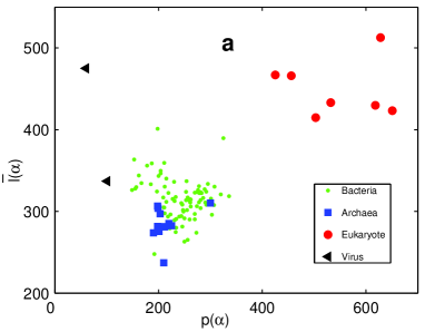
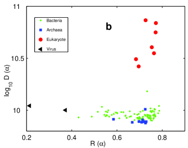
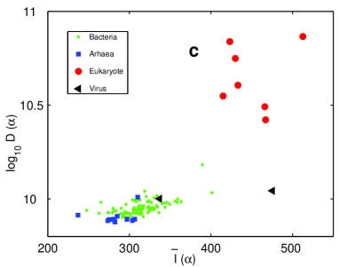
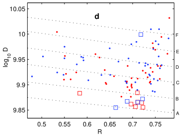
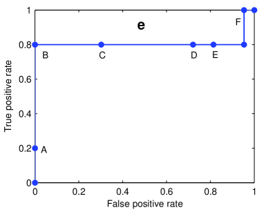
Figure 6: Classification of life based on cluster analysis of protein length distributions. a, The distributions of species in $p-\bar{l}$ plane. b, The distributions of species in $R-\log_{10}D$ plane. c, The distributions of species in $\bar{l}-\log_{10}D$ plane. d, Cross-validation analysis of the classification between Bacteria and Archaea by the distribtion in $R-\log_{10}D$ plane. The species in group $G_{1}$ are red, and the others in $G_{2}$ are blue. e, The cross-validated ROC curve shows the validity of the classifier.

Firstly, we studied the distribution of species in $\bar{l}-p$ plane, where $\bar{l}$ and $p$ only depend the data of the species’s own. We found that the groups of species in Bacteria, Archaea and Eucarya cluster together in three regions respectively (Fig. 6a). The archaea cluster in a small region where $\bar{l}$ and $p$ are relatively small; the bacteria cluster in a region where $\bar{l}$ and $p$ are relatively middle; and the eukaryotes cluster in a region where $\bar{l}$ and $p$ are relatively large. Thus, we have a new method to classify life. If the protein length distribution of a species is known but its classification if unclear, we can calculate average protein length $\bar{l}$ and peak number $p$ of this species. Then we can determine which domain the species belongs to according to its position in the $\bar{l}-p$ plane. Generally speaking, there is a correlation for the three domains: large $p$ corresponds to large $\bar{l}$. Such a correlation, however, is invalid for the species in the same domain. The relationship between $p$ and the genome size $s$ is much closer than the relationship between $p$ and average protein length $\bar{l}$ (Comparing Fig. 2a and Fig. 6a). If considering only one quantity, either $\bar{l}$ or $p$, we can not separate archaea from bacteria.

Secondly, we studied the distribution of species in $R-\log_{10}D$ plane, where $R$ and $D$ depend the data of other species according to their definitions, where the groups of species in three domains also cluster together respectively (Fig. 6b). The cluster of eukaryotes is separated obviously. The small region of the archaea borders on the big region of Eubacteria, so Archaea and eubacteria can still be separated. In the above, we chose the parameter $q=1/4$ in the definition of Minkowski distance $d(\alpha,\beta)$ and accordingly calculate the average Minkowski distance $D$. According to this choice of parameter $q$, we can separate the three domains more easily only by the average Minkowski distance $D$. The results are alike if varying $q$ from $1/2$ to $1/8$ in calculating $D$.

At last, we studied the distribution of species in other plots. According to the distributions of species in the plots of $\bar{l}-R$, $\bar{l}-\log D$ and $D-p$, we found that the groups of species in three domains still cluster together in the corresponding plots respectively (Fig. 6c).

Cross-validated ROC analysis. The cross-validated receiver operating characteristic (ROC) analysis can be taken as an objective measure to check for the quality of the above cluster analysis [33]. For instance, we can check the validity of the method in the cluster analysis between Bacteria and Archaea by $R$ and $\log_{10}D$ in the following. We found that the cross-validated ROC curves deviate from the diagonal line obviously, which shows the validity of our methods to cluster species according to the properties of their protein length distributions (Fig. 6d).

The method to draw the cross-validated ROC curve is as follows in detail. Firstly, we randomly separated the species in PEP into two groups $G_{1}$ and $G_{2}$. There are $42$ bacteria, $7$ archaea, $3$ eukaryotes and $1$ viruses in group $G_{1}$ and the remaining $53$ species are in group $G_{2}$ (Fig. 6d). Only based on the biological data of the species in $G_{1}$, we can define corresponding average correlation coefficient $R^{*}$ and average Minkowski distance $D^{*}$. According to the distribution of species in $G_{1}$ in the $R^{*}-\log_{10}D^{*}$ plane, the boundary between Bacteria and Archaea can be marked according to the distributions $(R^{*},\ \log_{10}D^{*})$ for the species in $G_{1}$. Then we can calculate the correlation coefficient $r(\alpha,\beta)$ and Minkowski distance $d(\alpha,\beta)$ between each of the species $\alpha\in G_{2}$ and the species $\beta\in G_{1}$, and accordingly obtain their average values for each species $\alpha\in G_{2}$

$$R^{**}(\alpha)=\frac{1}{53}\sum_{\beta\in\mbox{\tiny G}_{1}}r(\alpha,\beta)$$ (24)

$$D^{**}(\alpha)=\frac{1}{53}\sum_{\beta\in\mbox{\tiny G}_{1}}d(\alpha,\beta).$$ (25)

Still in the $R^{*}-\log_{10}D^{*}$ plane, we obtained a group of dots $(R^{**},\ \log_{10}D^{**})$ for species in $G_{2}$. Some of the archaea in $G_{2}$ still belong to the region of archaea according to the boundary defined by the data of species in $G_{1}$, while other archaea in $G_{2}$ cross the boundary. We can obtain the cross validated ROC curve according to the validity of cluster analysis for the species in $G_{2}$ by shifting the position of the boundary (Fig. 6e). We can repeat the above procedure after changing over the data between $G_{1}$ and $G_{2}$. Then we obtained another cross-validated ROC curve.

7 Spectral analysis of protein length distributions

Characteristics of power spectrum. The evolution of protein length is a virgin field in the study of molecular evolution. Although the mechanism of the evolution of protein length is unknown, we observed order in the protein lengths such as the quasi-periodicity, long range correlation and the tendency for conservation of protein length in domains. In this paper, we try to study the properties of protein length distributions by spectral analysis. In the section of “Definitions and notations”, we defined a power spectrum $\mathbf{y}(\alpha)$ for any species $\alpha$. We defined the characteristic frequency $f_{c}$ and the maximum frequency $f_{m}$, and we also defined the characteristic period $L_{c}$ and minimum period $L_{m}$ of the protein length distribution. For the domains Bacteria, Archaea and Eucarya, we defined the average power spectra $\mathbf{y}^{b}$, $\mathbf{y}^{a}$ and $\mathbf{y}^{e}$ respectively. Considering additional quantities such as average protein length $\bar{l}$, peak number $p$ and non-coding DNA content $\eta$, we observed some interesting correlations among these quantities. We show that there are correlations between protein lengths at different scales.

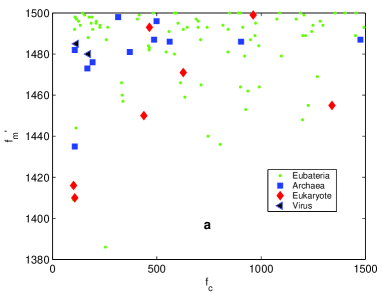
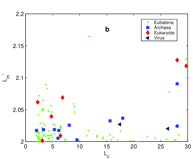
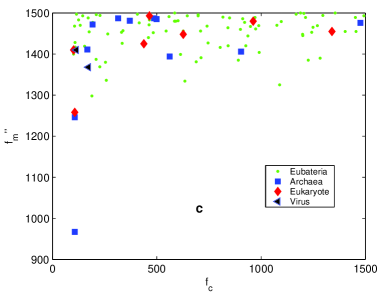
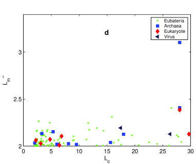
Figure 7: The protein length hierarchy. We choose $n_{p}=80$ ($n_{p}=30$) top highest peaks to find the largest frequency $f_{m}^{\prime}$ ($f_{m}^{\prime\prime}$) of obvious peaks, and consequently obtaining $L_{m}^{\prime}$ ($L_{m}^{\prime\prime}$). a $f_{m}^{\prime}$ approximately increases with $f_{c}$ for Archaea and Eukarya. b $L_{m}^{\prime}$ approximately increases with $L_{c}$ for Archaea and Eukarya. c $f_{m}^{\prime\prime}$ varies with $f_{c}$ in waves for Archaea and Eukarya. d $L_{m}^{\prime\prime}$ varies with $L_{c}$ in waves for Archaea and Eukarya. .

The protein length hierarchy. Structures can be observed in the fluctuations of the protein length distributions. We found that there are correlations between the characteristic frequency $f_{c}$ and maximum frequency $f_{m}$ (Fig. 7a, 7c). The characteristic frequency $f_{c}$ increases with the maximum frequency $f_{m}$, which is especially obvious for archaea and eukaryotes. There is also correlation between characteristic period $L_{c}$ and the minimum period $L_{m}$ (Fig. 7b, 7d). The values of $L_{c}$ and $L_{m}$ are intrinsic properties of protein length distributions that are free from the choice of cutoff $m$. Hence we found that the characteristic period $L_{c}$ increases with the minimum period $L_{m}$, especially for archaea and eukaryotes. Such an intrinsic correlation between $L_{c}$ and $L_{m}$ shows that there is a hierarchy in protein lengths. There might be a general mechanism in the organization of protein segments, which results in that the long protein length period $L_{c}$ varies with the short protein length period $L_{m}$ for individual species.

The constraint on average protein length. Comparing the fact that genome sizes range more than $1,000,000$-fold in the species on the planet, the average protein lengths in proteomes (several hundreds a.a.) vary slightly. There is a tendency for conservation of protein length in Bacteria, Archaea and Eucarya respectively [2] [3]. The average protein lengths in proteomes for Bacteria range from about $250$ a.a. to about $350$ a.a.; the values for Archaea are a little smaller; the values for Eucaryotes are around $500$ a.a.. The protein lengths vary slightly while the genome size evolves rapidly. Such a sharp contrast awaits answers. One possible solution is based on the understanding of evolutionary outlines of genome size and gene number from the beginning of life $t\approx-3,800$ Myr to present $t=0$. According to the theory in Ref. [20], we can obtain a formula of the evolutionary outline of average protein length

$$\bar{l}(t)=\left\{\begin{array}[]{llr}\frac{(1-\eta_{1}(t))s_{1}(t)}{3N_{1}(t)}&=242\exp(-\frac{t}{5320}),&t<T_{c}\\ \frac{(1-\eta_{2}(t))s_{2}(t)}{3N_{2}(t)}&=(110-14.3t)\exp(\frac{t}{164}),&t>T_{c}\end{array}\right.,$$ (26)

where the subscripts denote two stages in the evolution. This formula can explain the difference between genome size evolution and protein length evolution. Genome size increased rapidly, while the average protein length varied slightly and it even tended to decrease in each stage of the evolution. Our results agree with experimental observations in principle. The genome size was approximately proportional to the gene number before the time $T_{c}$, so the average protein lengths for prokaryotes should approximately keep constant in most time before $T_{c}$. Then both evolutionary speeds for gene number and genome size of eukaryotes shifted to new values after $T_{c}$, while the coding DNA content $1-\eta$ began to decrease. Such a transition of evolution of genome size and gene number around $T_{c}$ can set an upper limit for the average protein lengths for eukaryotes in the following evolution. The constraint on protein lengths could also be explained in an alternative way. The spectral analysis of protein length distributions might be helpful for us to understand the intrinsic mechanism of protein length evolution in detail. According to the relationship between $f_{c}$ and $\eta$ and the relationship between $f_{c}$ and $\bar{l}$, we can relate the evolution of average protein length $\bar{l}$ to the non-coding DNA content $\eta$, i.e., $\bar{l}$ tended to decrease when $\eta$ increased gradually. So the correlation of protein lengths can intrinsically constrain the average protein lengths in a certain range in the evolution.

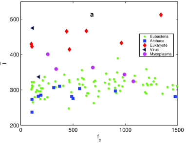
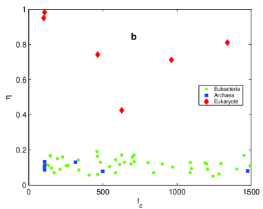
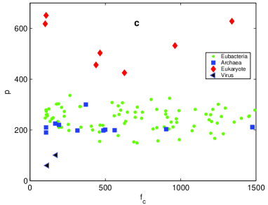
Figure 8: Explanation of the constraint on the average protein lengths. a, The rain-bow like distributions of species in three domains. The arc of Archaea is at lowest; the arc of Eubacteria is in the middle; and the arc of Eukarya is on the top. Mycoplasmas also form an arc. b, The relationship between $\eta$ and $f_{c}$. The V-shaped distribution of Eukaryotes is obvious. c, The relationship between $p$ and $f_{c}$. The V-shaped distribution of Eukaryotes is also obvious, and the distributions of Archaea and Eubacteria form flat arc respectively.

The distribution of species in $f_{c}-\eta$ plane shows a regular pattern: the value of $f_{c}$ tends to go from middle frequency to either lower frequency or higher frequency when $\eta$ increases gradually from about $0.1$ to $1$ (Fig. 8b). The same tendency of $f_{c}$ can be observed in $f_{c}-p$ plane (Fig. 8c) when $p$ increases gradually. The tendency of $f_{c}$ can be observed clearly especially according to the distributions of eukaryotes in the above. The mechanism constraining the average protein length can be inferred by the rainbow-like distribution of species in $f_{c}-\bar{l}$ plane, where the species in Bacteria, Archaea and Eucarya gathered in three horizontal convex arches respectively (Fig. 8a). Such an order shows that the average protein length $\bar{l}$ tends to evolve from long (corresponding middle $f_{c}$) to short (corresponding lower or higher $f_{c}$). We can observe directly that $\bar{l}$ decreases when $\eta$ increases (Fig. 3e), whose intrinsic mechanism, however, should be revealed by spectral analysis.

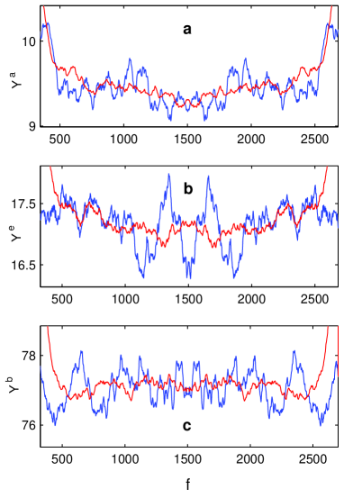
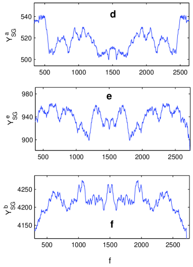
Figure 9: The profiles of total power spectra for three domains. After smoothing, the bottoms of total power spectra are convex for Archaea and Eucarya but concave for Bacteria. a-c, Smoothing by averaging in neighboring sections. Neighboring section $w_{1}=100$ (Blue) and $w_{2}=300$ (Red). d-f, Smoothing by Savitzky-Golay method (span=501, degree=2).

Average power spectra and phylogeny of three domains. We can study the properties of average power spectrum for Bacteria, Archaea and Eucarya respectively, which reflects the phylogeny of three domains. An important characteristic can be observed that the bottoms of the profiles of the average power spectra are either “convex” or “concave”. According to the results by several different ways to smooth the average power spectra $\mathbf{y}^{b}$, $\mathbf{y}^{a}$ and $\mathbf{y}^{e}$, we always concluded that the profiles of the average power spectra of Archaea and Eucarya have “convex bottoms” while the profile of the average power spectrum of Bacteria has “concave bottom”, where the “bottom” refers to the profile of power spectrum at $f$ around $m/2$ (Fig. 9). It is well known that the relationship between Archaea and Eucarya is closer than the relationship between Archaea and Bacteria. So the property of the outlines of the average spectra agrees with the phylogeny of the three domains. A convex bottom indicates that the power spectrum in the high frequency sector (at $f\sim 1500$) prevails the power spectrum in the low frequency sector (at $f\sim 500$); while a concave bottom indicates the opposite case. So the differences in the “bottoms” of power spectra of three domains might result from the underlying mechanism of protein length evolution.

In the above, the outlines of the average power spectra are obtained by smoothing the average power spectra in two methods. In the first method, we can smoothen $\mathbf{y}^{b}$, $\mathbf{y}^{a}$ and $\mathbf{y}^{e}$ as followings:

$$\mathbf{[}Y^{b}(w)]_{f}=\frac{1}{2w+1}\sum_{k=f-w}^{f+w}(y^{b})_{k}$$ (27)

$$\mathbf{[}Y^{a}(w)]_{f}=\frac{1}{2w+1}\sum_{k=f-w}^{f+w}(y^{a})_{k}$$ (28)

$$\mathbf{[}Y^{e}(w)]_{f}=\frac{1}{2w+1}\sum_{k=f-w}^{f+w}(y^{e})_{k},$$ (29)

where $2w+1$ is the width of the averaging sector and the range of $f$ is $f=1+w,...,m-w$. We obtain two sets of outlines of the average power spectra $\mathbf{Y}^{b}(w)$, $\mathbf{Y}^{a}(w)$ and $\mathbf{Y}^{e}(w)$ ($w=w_{1}=100$ or $w=w_{2}=300$) in the averaging calculations (Fig. 9a-9c). In the second method, we use the Savitzky-Golay method [34] to obtain outlines of the average power spectra $\mathbf{y}_{SG}(\alpha)$ for each species. Then, we averaged $\mathbf{y}_{SG}(\alpha)$ for Bacteria, Archaea and Eucarya respectively and denote the results as $\mathbf{Y}^{b}_{SG}$, $\mathbf{Y}^{a}_{SG}$ and $\mathbf{Y}^{e}_{SG}$ (Fig. 9d-9f). We found that all the outlines $\mathbf{Y}^{b}(s_{1})$, $\mathbf{Y}^{b}(s_{2})$ and $\mathbf{Y}^{b}_{SG}$ for Bacteria have concave bottoms and the corresponding outlines for Archaea and Eucarya have convex bottoms.

8 Conclusion and discussion

We conclude that the classification of life can be studied according to the understanding of fundamental mechanism of genome size evolution. The phylogenetic relationship among species in a domain is circular rather than the traditional concept of branching trees. The phylogenetic circle is a global property of living systems at the level of domain. We propose a natural criterion to define a domain by each of the phylogenetic circles. We observed at least three main phylogenetic circles corresponding to three known domains. In the global scenario of phylogenetic circles, we can explain the driving force in genome size evolution and the patterns of genome size distributions. The peak number $p$ plays the role of net driving force in genome size evolution. The genome size concerns two factors: (i) the net driving force $p$, and (ii) the circular phylogenetic relationship in a domain. Thus, there is no trivial correlation between genome size and biological complexity. The global circular relationship is quite different from the local branching relationship. The underlying mechanism in origin and evolution of life should consider that a domain should evolve as a whole.

There is rich evolutionary information stored in the fluctuations of protein length distributions. In the past, the fluctuations in protein length distribution were routinely assumed as random ones in a smooth background. Such a prejudice may result in the neglect of the pivotal evolutionary information stored in the fluctuations of protein length distributions. Based on the biological data of protein lengths in a proteome, we can calculate the genome size as well as the ratios of coding DNA and non-coding DNA for a species. Our results agree with the biological data very well. So there is profound relationship between the evolution of non-coding DNA and the evolution of coding DNA. We reconfirm the three-domain classification of life by cluster analysis of protein length distributions. We found that there are correlations between long periods and short periods of protein length distributions. The validity of our results can be verified by objective measures, which shouldn’t be ascribed to accidental coincidences. The study on protein length distributions provides us a chance to understand the macroevolution of life.

There should be a universal mechanism which underlies the molecular evolution. The fluctuations in protein length distributions may result from this universal mechanism. Thus we can determine the position of a species in the evolution of life by correlation analysis of the protein length distributions, and therefore obtain a panorama of evolution of life. There are many analogies between protein language and natural language of human being. We conjecture that linguistics may play a central role in the protein length evolution. A linguistic model was made to study the protein length evolution. In this model, protein sequences can be generated by grammars, hence we can obtain simulated protein length distributions for a set of grammars. The average protein lengths $\bar{l}$ and the peak numbers $p$ can be calculated consequently. The correlation between peak numbers $p$ and average protein length $\bar{l}$ in experimental observation can be explained by the simulation. Our results indicate an intrinsic relationship between the complexity of grammars in protein sequences and the peak numbers in protein length distributions.

Figure 3: The mechanism of genome evolution can be inferred by the circular distribution of species in $\Delta l-p$ plane. a, The phylogenetic circles consisted of species in Archaea, Eukarya, Eubacteria and Mycoplasma. The fundamental relationship goes round in circles in each domain. b, Species only distribute in the left and right quadrants. The origin $O$ is at $s^{*}\sim 3.5\times 10^{6}$ bp. c, The approximate proportional relation between $\bar{l}$ and $\Delta l$ (Correlation coefficient is $0.9022$). d, The distribution of species in $s-\bar{l}$ plane. e, The coarse linear relation between $\bar{l}$ and $\eta$ in each domain. f, The distribution of species in $s-\eta$ plane. g, The distribution of species in $\theta-\eta$ plane. h, The distribution of species in $\log_{10}N-\Delta l$ plane. h, Relationship between non-coding DNA ratio and protein length standard error.

Figure 4: Phylogenetic circles in $\Delta l-p$ plane and bifurcated distribution in $\Delta l-s$ plane. The abbreviation of the names of groups of species are as follows: Euryarchaeota (EA), Crenarchaeota (CA), Alphaproteobacteria (P$\alpha$), Betaproteobacteria (P$\beta$), Gammaproteobacteria (P$\gamma$), Deltaproteobacteria (P$\delta$), Epsilonproteobacteria (P$\epsilon$), Firmicutes (Fir), Acidobacteria (Aci), Actinobacteria (Act), Cyanobacteria (Cya), Bacteroidetes/Chlorobi (Chl), Spirochaetes (Spi), Chlamydiae/Verrucomicrobia (Ver), Chloroflexi (Cho), Deinococcus-Thermus (Dei), Thermotogae (The). a, Phylogenetic circles formed by $775$ microbes in NCBI. b, The phylogenetic circle formed by phyla of eubacteria. c, The phylogenetic circle formed by proteobacteria. d, Bifurcated distribution of species in $\Delta l-s$ plane. e, Bifurcated distribution of proteobacteria.

Table 1: The values of properties for species

No.	$\bar{l}$	$\Delta l$	$L_{c}$	$p$	$\theta$	$\eta$	$S$	$N$	$R$	$D$
1	358.83	254.48	2.50	187	0.4960			683	0.56	9.98
2	314.91	204.75	5.08	261	0.2571			3322	0.75	9.94
3	237.08	170.15	28.04	210	0.4874	0.1088	1669695	2694	0.58	9.91
4	307.82	201.72	4.89	307	0.2173	0.1170	5674062	5402	0.77	9.94
5	313.81	188.23	2.47	281	0.2238			5274	0.76	9.95
6	317.02	187.64	3.56	209	0.3620	0.0700	1551335	1522	0.68	9.91
7	433.07	293.16	3.12	532	0.2096	0.7120	115409949	25541	0.75	10.61
8	275.47	182.87	6.01	201	0.2996	0.0780	2178400	2406	0.73	9.89
9	262.96	189.58	4.30	250	0.2681	0.1590	5370060	5311	0.75	9.92
10	273.88	190.36	13.16	273	0.2452	0.1600	546909	5274	0.76	9.93
11	290.35	203.62	4.64	270	0.2428	0.1300	4214810	4099	0.76	9.92
12	389.55	265.58	3.24	325	0.2617			4776	0.73	10.18
13	304.71	221.93	14.35	211	0.3886			1482	0.66	9.94
14	330.38	223.17	3.37	212	0.4112			1141	0.64	9.95
15	324.15	221.99	9.06	292	0.2575			3584	0.75	9.99
16	322.27	187.75	28.30	279	0.2649			4986	0.74	9.95
17	333.31	225.12	2.34	185	0.4649	0.0630	1443725	850	0.59	9.96
18	326.10	197.07	3.03	276	0.2744			4184	0.73	9.94
19	323.53	193.58	3.33	275	0.6183			3446	0.43	9.93
20	312.96	197.49	17.05	302	0.1805			8307	0.79	9.99
21	293.74	207.45	6.21	218	0.3146	0.1300	3294935	2059	0.72	9.91
22	328	208.60	6.48	155	0.5060	0.1640	618000	574	0.55	9.95
23	326.21	209.97	4.23	149	0.5028			546	0.56	9.95
24	329.71	208.28	3.53	157	0.5092			504	0.55	9.94
25	414.83	291.03	6.45	503	0.1945	0.7419	97000000	21832	0.76	10.55
26	311.59	197.79	7.37	215	0.3441	0.0570	1641181	1633	0.69	9.92
27	334.59	210.69	2.45	167	0.5105			583	0.54	9.96
28	323.58	213.94	2.73	281	0.2471	0.0940	4016942	3737	0.75	9.99
29	346.45	242.84	3.67	204	0.4177			998	0.63	9.98
30	343.36	239.29	7.21	200	0.4590			907	0.60	9.98
31	279.99	217.23	22.56	234	0.4107	0.1110	2154946	2252	0.64	9.95
32	349.61	244.35	3.26	204	0.4502			894	0.60	9.97
33	311.15	206.49	2.01	278	0.2228	0.1100	4751080	4396	0.77	9.95
34	305.91	219.99	3.33	262	0.2442	0.1200	3940880	3847	0.76	9.95
35	313.70	213.96	2.07	253	0.2695	0.1690	3031430	2722	0.74	9.93

No.	$\bar{l}$	$\Delta l$	$L_{c}$	$p$	$\theta$	$\eta$	$S$	$N$	$R$	$D$
36	336.16	199.14	3.08	230	0.3379			2373	0.69	9.93
37	316.99	218.83	5.37	256	0.2937			2269	0.73	9.95
38	323.04	210.43	4.30	270	0.2943			2947	0.72	9.96
39	314.44	204.83	2.57	262	0.2645			2989	0.74	9.93
40	279.28	207.24	11.81	222	0.4060	0.1100	1995275	2009	0.64	9.93
41	308.32	196.77	2.14	246	0.2753	0.0910	3284156	3099	0.74	9.92
42	303.93	224.44	3.57	281	0.3107			3524	0.71	9.99
43	512.73	394.58	2.24	628	0.2562	0.8100	120000000	18358	0.73	10.87
44	316.53	206.93	2.31	286	0.2247	0.1220	4641000	4281	0.77	9.96
45	290.06	211.06	2.50	260	0.2852	0.1200	3218031	3145	0.74	9.95
46	315.67	203.56	2.40	301	0.2226			4463	0.77	9.95
47	310.10	230.72	3.09	244	0.3149	0.1020	2714500	2067	0.71	9.94
48	310.96	222.74	4.21	290	0.2462			4425	0.76	10.00
49	274.78	204.43	16.22	233	0.4102			1715	0.64	9.93
50	304.90	201.23	15.54	210	0.3434	0.1500	4524893	1709	0.69	9.92
51	285.21	187.56	15.63	220	0.3185			2058	0.71	9.91
52	336.99	285.66	17.44	101	0.6795			202	0.37	10.00
53	296.21	202.87	17.54	223	0.3495	0.0700	1799146	1874	0.69	9.93
54	317.57	239.38	2.49	233	0.3633			1564	0.68	9.96
55	423.24	365.33	28.04	651	0.1889	0.9830	3000000000	37229	0.77	10.84
56	312.62	204.01	3.20	231	0.3399			1813	0.70	9.92
57	293.62	205.33	2.52	240	0.3358	0.1260	2365589	2266	0.70	9.92
58	301.52	192.68	2.06	255	0.2637			3002	0.75	9.92
59	297.65	194.49	3.16	212	0.3320			2023	0.70	9.90
60	310.94	214.31	26.55	261	0.2837			3652	0.73	9.96
61	299.76	213.82	19.48	248	0.2748	0.0970	3011209	2968	0.74	9.92
62	301.67	197.80	29.70	247	0.2622	0.0970	2944528	2833	0.75	9.90
63	310.32	249.91	8.09	300	0.2999			4540	0.72	10.01
64	297.05	194.72	3.32	203	0.3418			1687	0.70	9.89
65	280.99	194.59	2.03	211	0.3228	0.0800	1751377	1873	0.72	9.89
66	281.17	194.61	2.03	212	0.3222			1869	0.72	9.89
67	429.90	345.14	29.70	618	0.1828	0.9500	2500000000	28085	0.77	10.75
68	475.19	373.68	26.32	60	0.8092			80	0.21	10.04
69	330.81	195.84	4.98	278	0.2537			4340	0.75	9.95
70	327.06	223.16	14.29	289	0.2451	0.0900	4345492	3906	0.75	9.98

No.	$\bar{l}$	$\Delta l$	$L_{c}$	$p$	$\theta$	$\eta$	$S$	$N$	$R$	$D$
71	401.18	276.95	11.63	198	0.5086			726	0.53	10.03
72	363.49	263.10	4.35	153	0.5416	0.1200	580070	484	0.52	9.98
73	324.39	233.57	2.79	197	0.5674			1016	0.49	9.94
74	343.90	241.56	3.03	162	0.4804			686	0.58	9.95
75	359.33	253	8.88	211	0.4867	0.0860	963879	778	0.56	10.00
76	283.77	210.78	4.78	226	0.3407	0.1710	2184406	2065	0.70	9.94
77	323.95	225.17	2.36	253	0.3436			2461	0.69	9.96
78	291.45	183.80	3.29	250	0.2513			3496	0.75	9.90
79	336.92	245.94	13.22	254	0.3800			1909	0.66	9.99
80	330.34	213.72	5.50	308	0.2167	0.1060	6264403	5563	0.77	10.01
81	322.36	204.90	24	283	0.2240			5316	0.76	9.99
82	303.72	187.29	5.34	199	0.3236			1764	0.71	9.88
83	281.55	180.80	6.16	198	0.3071			2065	0.72	9.89
84	273.67	177.40	28.04	190	0.3851			2064	0.67	9.88
85	320.74	234.60	3.73	320	0.2242	0.1270	5810922	5092	0.77	10.01
86	295.89	190.36	15.87	303	0.1953			7264	0.78	9.97
87	247.82	226.36	6.52	192	0.5019	0.1900	1268755	1374	0.57	9.94
88	466.99	341.69	4.78	425	0.3018	0.4250	13800000	4987	0.70	10.42
89	296.89	192.62	4.02	270	0.4419			4176	0.61	9.92
90	294.33	214.31	20.69	244	0.2845			2631	0.74	9.93
91	289.39	198.90	2.21	231	0.3210			2121	0.71	9.92
92	318.67	214.78	11.32	336	0.1809	0.1110	8670000	7894	0.79	10.04
93	281.36	218.89	4.05	246	0.3949			2094	0.66	9.94
94	290.80	202.47	4.72	234	0.3350			1845	0.70	9.92
95	282.32	171.30	17.96	225	0.3006			2977	0.73	9.88
96	306.57	195.54	9.52	198	0.3378	0.1300	1564905	1478	0.70	9.89
97	315.18	196.90	2.41	227	0.3316	0.0500	1860725	1846	0.70	9.92
98	340.13	222.99	2.75	215	0.4457			1031	0.60	9.98
99	356.08	272.04	5.13	178	0.5053	0.0700	751719	611	0.55	9.99
100	312.85	219.39	27.52	260	0.3336	0.1255	4034065	2736	0.70	9.96
101	306.37	212.27	27.78	274	0.2561			4800	0.75	9.99
102	322.57	205.70	6.45	219	0.3362	0.0600	2110355	2044	0.69	9.93
103	333.68	235.42	5.12	295	0.2545	0.1440	5175554	4029	0.75	10.02
104	265.15	231.31	26.09	256	0.4376	0.1200	2679305	2763	0.62	9.98
105	466.08	364.04	6.85	456	0.3221			6356	0.68	10.49
106	308.20	220.05	8.98	292	0.3265	0.1420	4653728	4087	0.70	9.99

Table 2: List of the species in PEP

(No. 1) Acholeplasma florum (Mesoplasma florum) DOMAIN: Eubacteria

(No. 2) Acinetobacter sp (strain ADP1) DOMAIN: Eubacteria

(No. 3) Aeropyrum pernix K1 DOMAIN: Archaebacteria

(No. 4) Agrobacterium tumefaciens (strain C58 / ATCC 33970) Eubacteria

(No. 5) Agrobacterium tumefaciens DOMAIN: Eubacteria

(No. 6) Aquifex aeolicus DOMAIN: Eubacteria

(No. 7) Arabidopsis thaliana DOMAIN: Eukaryote

(No. 8) Achaeoglobus fulgidus DOMAIN: Archaebacteria

(No. 9) Bacillus anthracis (strain Ames) DOMAIN: Eubacteria

(No. 10) Bacillus cereus (ATCC 14579) DOMAIN: Eubacteria

(No. 11) Bacillus subtilis DOMAIN: Eubacteria

(No. 12) Bacteroides thetaiotaomicron VPI-5482 DOMAIN: Eubacteria

(No. 13) Bartonella henselae (Houston-1) DOMAIN: Eubacteria

(No. 14) Bartonella quintana (Toulouse) DOMAIN: Eubacteria

(No. 15) Bdellovibrio bacteriovorus DOMAIN: Eubacteria

(No. 16) Bordetella bronchiseptica RB50 DOMAIN: Eubacteria

(No. 17) Borrelia burgdorferi DOMAIN: Eubacteria

(No. 18) Bordetella parapertussis DOMAIN: Eubacteria

(No. 19) Bordetella pertussis DOMAIN: Eubacteria

(No. 20) Bradyrhizobium japonicum DOMAIN: Eubacteria

(No. 21) Brucella melitensis; B melitensis; brume DOMAIN: Eubacteria

(No. 22) Buchnera aphidicola (subsp. Acyrthosiphon pisum) Eubacteria

(No. 23) Buchnera aphidicola (subsp. Schizaphis graminum) Eubacteria

(No. 24) Buchnera aphidicola (subsp. Baizongia pistaciae) Eubacteria

(No. 25) Caenorhabditis elegans DOMAIN: Eukaryote

(No. 26) Campylobacter jejuni DOMAIN: Eubacteria

(No. 27) Candidatus Blochmannia floridanus DOMAIN: Eubacteria

(No. 28) Caulobacter crescentus DOMAIN: Eubacteria

(No. 29) Chlamydophila caviae DOMAIN: Eubacteria

(No. 30) Chlamydia muridarum DOMAIN: Eubacteria

(No. 31) Chlorobium tepidum DOMAIN: Eubacteria

(No. 32) Chlamydia trachomatis DOMAIN: Eubacteria

(No. 33) Chromobacterium violaceum ATCC 12472 DOMAIN: Eubacteria

(No. 34) Clostridium acetobutylicum DOMAIN: Eubacteria

(No. 35) Clostridium perfringens DOMAIN: Eubacteria

(No. 36) Clostridium tetani DOMAIN: Eubacteria

(No. 37) Corynebacterium diphtheriae NCTC 13129 DOMAIN: Eubacteria

(No. 38) Corynebacterium efficiens DOMAIN: Eubacteria

(No. 39) Corynebacterium glutamicum DOMAIN: Eubacteria

(No. 40) Coxiella burnetii DOMAIN: Eubacteria

(No. 41) Deinococcus radiodurans DOMAIN: Eubacteria

(No. 42) Desulfovibrio vulgaris subsp. vulgaris str. Hildenborough Eubacteria

(No. 43) Drosophila melanogaster DOMAIN: Eukaryote

(No. 44) Escherichia coli DOMAIN: Eubacteria

(No. 45) Enterococcus faecalis DOMAIN: Eubacteria

(No. 46) Erwinia carotovora DOMAIN: Eubacteria

(No. 47) Fusobacterium nucleatum DOMAIN: Eubacteria

(No. 48) Gloeobacter violaceus DOMAIN: Eubacteria

(No. 49) Haemophilus ducreyi DOMAIN: Eubacteria

(No. 50) Haemophilus influenzae DOMAIN: Eubacteria

(No. 51) Halobacterium sp. (strain NRC-1) DOMAIN: Archaebacteria

(No. 52) Human cytomegalovirus (strain AD169) DOMAIN: virus

(No. 53) Helicobacter heilmannii DOMAIN: Eubacteria

(No. 54) Helicobacter pylori DOMAIN: Eubacteria

(No. 55) Homo sapiens DOMAIN: Eukaryote

(No. 56) Lactobacillus johnsonii DOMAIN: Eubacteria

(No. 57) Lactococcus lactis (subsp. lactis) DOMAIN: Eubacteria

(No. 58) Lactobacillus plantarum WCFS1 DOMAIN: Eubacteria

(No. 59) Leifsonia xyli (subsp. xyli) DOMAIN: Eubacteria

(No. 60) Leptospira interrogans (serogroup Icterohaemorrhagiae / serovar Copenhageni) DOMAIN: Eubacteria

(No. 61) Listeria innocua DOMAIN: Eubacteria

(No. 62) Listeria monocytogenes DOMAIN: Eubacteria

(No. 63) Methanosarcina acetivorans DOMAIN: Archaebacteria

(No. 64) Methanopyrus kandleri DOMAIN: Archaebacteria

(No. 65) Methanobacterium thermoautotrophicum DOMAIN: Archaebacteria

(No. 66) Methanobacterium thermoautotrophicum DOMAIN: Archaebacteria

(No. 67) Mus musculus DOMAIN: Eukaryote

(No. 68) Murine herpesvirus 68 strain WUMS DOMAIN: virus

(No. 69) Mycobacterium avium; M avium; mycav DOMAIN: Eubacteria

(No. 70) Mycobacterium bovis AF2122/97 DOMAIN: Eubacteria

(No. 71) Mycoplasma gallisepticum DOMAIN: Eubacteria
(No. 72) Mycoplasma genitalium DOMAIN: Eubacteria
(No. 73) Mycoplasma mycoides (subsp. mycoides SC) DOMAIN: Eubacteria
(No. 74) Mycoplasma pneumoniae DOMAIN: Eubacteria
(No. 75) Mycoplasma pulmonis DOMAIN: Eubacteria
(No. 76) Neisseria meningitidis DOMAIN: Eubacteria
(No. 77) Nitrosomonas europaea DOMAIN: Eubacteria
(No. 78) Oceanobacillus iheyensis DOMAIN: Eubacteria
(No. 79) Porphyromonas gingivalis DOMAIN: Eubacteria
(No. 80) Pseudomonas aeruginosa DOMAIN: Eubacteria
(No. 81) Pseudomonas putida DOMAIN: Eubacteria
(No. 82) Pyrococcus abyssi DOMAIN: Archaebacteria
(No. 83) Pyrococcus furiosus DOMAIN: Archaebacteria
(No. 84) Pyrococcus horikoshii DOMAIN: Archaebacteria
(No. 85) Ralstonia solanacearum DOMAIN: Eubacteria
(No. 86) Rhizobium loti DOMAIN: Eubacteria
(No. 87) Rickettsia conorii DOMAIN: Eubacteria
(No. 88) Schizosaccharomyces pombe DOMAIN: Eukaryote
(No. 89) Shigella flexneri Shigella flexneri DOMAIN: Eubacteria
(No. 90) Staphylococcus aureus DOMAIN: Eubacteria
(No. 91) Streptococcus agalactiae DOMAIN: Eubacteria
(No. 92) Streptomyces coelicolor DOMAIN: Eubacteria
(No. 93) Streptococcus pneumoniae DOMAIN: Eubacteria
(No. 94) Streptococcus pyogenes DOMAIN: Eubacteria
(No. 95) Sulfolobus solfataricus DOMAIN: Archaebacteria
(No. 96) Thermoplasma acidophilum DOMAIN: Archaebacteria
(No. 97) Thermotoga maritima DOMAIN: Eubacteria
(No. 98) Treponema pallidum DOMAIN: Eubacteria
(No. 99) Ureaplasma urealyticum DOMAIN: Eubacteria
(No. 100) Vibrio cholerae DOMAIN: Eubacteria
(No. 101) Vibrio parahaemolyticus RIMD 2210633 DOMAIN: Eubacteria
(No. 102) Wolinella succinogenes DOMAIN: Eubacteria
(No. 103) Xanthomonas axonopodis (pv. citri); X axonopodis (pv. citri) DOMAIN: Eubacteria
(No. 104) Xylella fastidiosa DOMAIN: Eubacteria
(No. 105) Saccharomyces cerevisiae DOMAIN: Eukaryote
(No. 106) Yersinia pestis DOMAIN: Eubacteria

References

- [1] Woese, C. R., Kandler, O., & Wheelis, M. L. Towards a natural system of organisms: proposal for the domains Archaea, Bacteria, and Eucarya. Proc. Natl. Acad. Sci. USA 87, 4576-4579 (1990).
- [2] Wang, D., Hsieh, M. and Li., W. H. A general tendency for conservation of protein length across eukaryotic kingdoms. Mol. Biol. Evol. 22, 142-147 (2005).
- [3] Xu, L. et al. Average gene length is highly conserved in prokaryotes and eukaryotes and diverges only between the two kingdoms. Mol. Biol. Evol. 23, 1107-1108 (2006).
- [4] Li., W. H. Molecular Evolution. Sinauer Associated, Sunderland, Mass. (1997).
- [5] Kinch, L. N. and Grishin, N. V. Evolution of protein stuctures and functions. Curr. Opin. Struct. Biol. 12, 400-408 (2002).
- [6] Akashi, H. Translational selection and yeast proteome evolution. Genetics 164, 1291-1303 (2003).
- [7] Berman, A. L., Kolker, E. and Trifonov, E. N. Unerlying order in portein sequence organization. Proc. Natl. Acad. Sci. USA 91, 4044-4047 (1994).
- [8] Kolker, E. et al. Spectral analysis of distributions: finding periodic components in Eukaryotic enzyme length data. J. of Integrative Biol. 6, 123-130 (2002).
- [9] Zainea, O. and Morariu, V. V. The length of coding sequences in a bacterial genome: Evidence for short-range correlation. Fluct. Noise Lett. 7, L501-L506 (2007).
- [10] Morariu, V. V. Microbial genome as a fluctuating system: Distribution and correlation of coding sequence lengths. arXiv Preprint Archive [online], http://arxiv.org/abs/0805.4315 (2008).
- [11] Gimona, M. Protein linguistics - a grammar for modular protein assembly? Nat. Rev. Mol. Cell Biol. 7, 68-73 (2006).
- [12] Searls, D. B. Language of genes. Nature 420, 211-217 (2002).
- [13] Hertzsprung, E. Zur strahlung der sterne. Zeitschrift für wissenschaftliche Photographie 3, 429-442 (1905).
- [14] Russell, H. N. “Giant” and “dwarf” stars. Observatory 36, 324-329 (1913).
- [15] Carter, P., Liu, J. and Rost, B. PEP: Predictions for Entire Proteomes. Nucl. Acids Res. 31, 410-413 (2003). The URL of the database PEP is http://cubic.bioc.columbia.edu/pep.
- [16] Taft, R. J. and Mattick, J. S. Increasing biological complexity is positively correlated with the relative genome-wide expansion of non-protein-coding DNA sequences. arXiv Preprint Archive [online], http://arxiv.org/abs/q-bio.GN/0401020 (2004).
- [17] International Human Genome Sequencing Consortium, Initial sequencing and analysis of the human genome. Nature 409, 860-921 (2001).
- [18] Gregory T. R. ed. The evolution of the genome (Elsevier, Amsterdam, 2005).
- [19] Gregory T. R. Macroevolution, hierarchy theory, and the C-value enigma. Paleobiology 30, 179-202 (2004).
- [20] Li, D. J., & Zhang, S. The C-value enigma and timing of the Cambrian explosion. arXiv Preprint Archive [online], http://arxiv.org/abs/0806.0108 (2008).
- [21] Croft, L. J., Lercher, M. J., Gagen, M. J. & Mattick, J. S. Is prokaryotic complexity limited by accelerated growth in regulatory overhead. arXiv Preprint Archive [online], http://arxiv.org/abs/q-bio.MN/0311021 (2003).
- [22] Sayers, E. W. Database resources of the National Center for Biotechnology Information. Nucleic Acids Res. 37, D5-15 (2009).
- [23] Benson, D. A. et al. GenBank. Nucleic Acids Res. 37, D29-31 (2009).
- [24] Knoll, A. H. and Carroll, S. B. Early animal evolution: emerging views from comparative biology and geology. Science 284, 2129-2137 (1999).
- [25] Woese, C. R. On the evolution of cells. Proc. Natl. Acad. Sci. USA 99, 8742-8747 (2002).
- [26] Leitch, I. J., Soltis, D. E., Soltis, P. S. and Bennett, M. D. Evolution of DNA Amounts Across Land Plants (Embryophyta). Anal. Botany 95, 207-217 (2005).
- [27] Bowers, J. E. et al. Unravelling angiosperm genome evolution by phylogenetic analysis of chromosomal duplication events. Nature 422, 433-438 (2003).
- [28] Lynch, M. and Conery, J. S. The evolutionary fate and consequences of duplicate genes. Science 290, 1151-1155 (2000).
- [29] Wolfe, K. H. Yesterday s polyploids and the mystery of diploidization. Nat. Rev. Genet. 36, 333-341 (2001).
- [30] Vitte, C. and Bennetzen, J. L. Analysis of retrotransposon structural diversity uncovers properties and propensities in angiosperm genome evolution. Proc. Natl. Acad. Sci. USA 103, 17638-17643 (2006).
- [31] Morariu, V. V. A limiting rule for the variability of coding sequences length in microbial genomes. arXiv Preprint Archive [online], http://arxiv.org/abs/0805.1289 (2008).
- [32] Destri, C. and Miccio, C. A simple stochastic model for the evolution of protein lengths. arXiv Preprint Archive [online], http://arxiv.org/abs/q-bio/0703054v2 (2007).
- [33] Fawcett, T. An introduction to ROC analysis. Pattern Recognition Lett. 27 861-874 (2006).
- [34] Savitzky, A. and Golay, M. J. E. Smoothing and differentiation of data. Anal. Chem. 36, 1627-1639 (1964).