Double-quantum-coherence attosecond x-ray spectroscopy of spatially separated, spectrally overlapping core-electron transitions

Abstract

X-ray four-wave mixing signals generated in the $\boldsymbol{k}_{1}+\boldsymbol{k}_{2}-\boldsymbol{k}_{3}$ phase-matching direction are simulated for N1s transitions in para-nitroanline and two-ring hydrocarbons disubstituted with an amine and a nitroso groups. The two-dimensional x-ray correlation spectra (2DXCS) provide background-free probes of couplings between core-electron transitions even for multiple core shells of the same type. Features attributed to couplings between spatially-separated core transitions connected by delocalized valence excitations provide information about molecular geometry and electronic structure unavailable from linear near-edge x-ray absorption (XANES).

I Introduction

Near-edge x-ray absorption spectroscopy (XANES) provides a powerful frequency-domain probe for electronic structure of molecules.Stohr (1996) Transitions from the ground state to bound core-excited states appear as resonances in the absorption spectrum below the ionization edge. Because of the compactness of core shells, the positions and intensities of XANES peaks arising from a given shell carry information about the electronic structure in its vicinity. XANES carries characteristic signatures of the electronic environment of the absorbing atom. If two atoms are spatially well separated, their contribution to XANES is essentially additive. The molecular structure can then be elucidated by identifying the signatures of various functional groups in the total XANES spectra. This additivity, known as the building-block principle of XANESStohr (1996), makes it insensitive to electronic-structure variations away from the absorbing atoms as well as to subtle differences in molecular geometry.

Coherent nonlinear x-ray spectroscopies can overcome these limitations and extend the XANES capabilities towards more detailed probes of electronic and molecular structure. Coherent nonlinear measurements performed with infrared and visible femtosecond phase-locked pulse sequences, can enhance desired spectral features, eliminate certain line-broadening mechanisms, and detect interferences between specific quantum pathways contributing to the optical response.Mukamel (2000); Mukamel and Hochstrasser (2001); Jonas (2003); Engel et al. (2007); Hochstrasser (2007); Li et al. (2006); Chernyak et al. (1998); Zhang et al. (1999) The ongoing development of high-harmonic generation (HHG) and forth-generation synchratron sources based on the x-ray free-electron laser (XFEL) (see Refs. Bucksbaum, 2007; Goulielmakis et al., 2007; Kapteyn et al., 2007 and references therein) provide first steps towards the realization of coherent nonlinear measurements in the x-ray domain. These will require multiple x-ray pulses with controlled timing, phases and sufficient intensity.

As these sources continue to develop, one may rely on theoretical simulations to design and evaluate possible nonlinear techniques. Earlier studies focused on ultrafast x-ray absorption and scattering in systems prepared by an optical pulseBrown et al. (1999); Gel’mukhanov et al. (2000); Privalov et al. (2003); Bressler and Chergui (2004); Campbell and Mukamel (2004). Tanaka and Mukamel studied frequency-domain all-x-ray four-wave mixingTanaka and Mukamel (2002a, b). Pump-probe is the simplest time-domain nonlinear experiment. This incoherent technique requires two pulses with variable time delay but no control over the phases. Combinations of optical pump (either visible Privalov et al. (2003); Guimaraes et al. (2004); Tanaka and Mukamel (2004) or infraredFelicissimo et al. (2005); Guimaraes et al. (2005); Liu et al. (2008)) and x-ray probe as well as x-ray pump/x-ray probeTanaka and Mukamel (2003); Schweigert and Mukamel (2007a) have been studied. We consider on attosecond phase-coherent four-wave-mixing techniques which require up to four x-ray beams.Mukamel (2005); Schweigert and Mukamel (2007b) These offer a much higher degree of control of the observed dynamical processes and could result in qualitatively new information unavailable from any other technique. In an earlier study, we have examined the $\boldsymbol{k}_{I}=-\boldsymbol{k}_{1}+\boldsymbol{k}_{2}+\boldsymbol{k}_{3}$ 2DXCS signal of aminophenol obtained by varying two delay periods in the coherent x-ray four-wave mixing measurement.Schweigert and Mukamel (2007b, 2008a) The simulated two-color 2DXCS signal where two pulses are tuned to the N K-edge and the other two to the O K-edge was shown to be highly sensitive to the coupling of the spatially- and spectrally-separated core transitions. Distinct off-diagonal cross peaks appear due to the interference among quantum pathways that involve only singly core-excited states (excited-state stimulated emission [ESE] and ground-state bleaching [GSB]) and pathways that involve singly and doubly core-excited states (excited-state absorption, ESA). If the frequency of a given core-shell transition is independent of whether another core-shell is excited, the ESA contribution interfers destructively with the ESE and GSB and the cross peaks vanish. The coupling between two transitions results in a distinct 2DXCS cross-peak pattern. In constrast, XANES of two independent transitions is exactly the sum of the individual transition. Since the coupling between two core transitions depends on the distance between the two core shells as well as the electronic structure in their vicinity, 2DXCS cross peaks carry a wealth of qualitatively new information beyond XANES.

The simulated $\boldsymbol{k}_{I}$ signal of aminophenol has a simple structure because the 100 eV separation between the N 1s and O 1s transitions is much larger than the assumed pulse bandwidths ($<$ 10 eV). The two-color 2DXCS signal thus involves transitions from both cores and the resulting spectrum contains no diagonal peaks. Here we focus on a homonuclear 2DXCS signal in systems with multiple core shells of the same type. In this case, both transitions involving two different or the same core-shells contribute to the signal since the chemical shifts (a few eV) are smaller than the pulse bandwidths and the 2DXCS diagonal and cross peaks spectrally overlap. Due to interference, the latter are usually weaker. A higher spectral resolution is thus required to separate the cross peaks and extract the couplings. The $\boldsymbol{k}_{I}$ signal of nucleobases and their pairs was shown to be dominated by a strong GSB contribution arising from transition of imine N 1s into the $\pi$ orbitals of the heterocycle.Healion et al. (in press)

In this paper, we show that the single-resonance contributions can be eliminated by monitoring the 2DXCS signal in the $\boldsymbol{k}_{III}=\boldsymbol{k}_{1}+\boldsymbol{k}_{2}-\boldsymbol{k}_{3}$ direction. This technique Scheurer and Mukamel (2001) corresponding to double-quantum coherence in NMRErnst et al. (1987) was already predicted to show high sensitivity to exciton coupling in the infrared Cervetto et al. (2004); Fulmer et al. (2004); Zhuang et al. (2005) and the visibleLi et al. (2008); Abramavicius et al. (2008). Within the rotating-wave approximation, only two ESA pathways contribute to this signal, both involving doubly core-excited states. When two core transitions are independent the two pathways intefere destructively. This signal thus contains only features induced by the coupling between core transitions.

In Section II we employ the response-function formalism Mukamel (1995) to derive the sum-over-states expression for the $\boldsymbol{k}_{III}$ signal. The $\boldsymbol{k}_{I}$ and $\boldsymbol{k}_{III}$ signals of a model four-level system with and without coupling between the two core transitions are compared in Section III. In Section IV we present the N1s XANES and $\boldsymbol{k}_{III}$ 2DXCS signals of benzene, stilbene, and biphenyl disubstituted with the amine and nitroso groups (Fig. 1). The relevant core-excited states are described using singly- and doubly-substituted Kohn-Sham determinants within the equivalent-core approximation Schweigert and Mukamel (2008a). The results are summarized in Section V.

II Sum-over-states expressions for the $\boldsymbol{k}_{1}+\boldsymbol{k}_{2}-\boldsymbol{k}_{3}$ signal

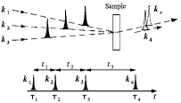
Figure 2: Pulse sequence in a 2DXCS experiment. Three pulses $\boldsymbol{k}_{1}$, $\boldsymbol{k}_{2}$, and $\boldsymbol{k}_{3}$ induce a core-hole polarization in the molecule, which is probed by the heterodyne field $\boldsymbol{k}_{4}$. The time intervals $t_{3}$, $t_{2}$, $t_{1}$ between consecutive pulses serve as control parameters.

The most general four-wave-mixing experiment uses a sequence of four soft x-ray pulses (Fig. 2). Possible experiments with fewer pulses are discussed below.

$$\boldsymbol{E}(\boldsymbol{r},t)=\sum_{j}^{4}\big{[}\boldsymbol{e_{j}}\mathcal{E}_{j}(t-\tau_{j})e^{i\boldsymbol{k}_{j}\boldsymbol{r}-i\omega_{j}(t-\tau_{j})}+c.c.\big{]}$$ (1)

Here, $\mathcal{E}_{j}(\tau)$ is the complex (positive frequency) temporal envelope of the $j$’th pulse, $\boldsymbol{e_{j}}$ is the polarization, $\boldsymbol{k}_{j}$ is the wavevector, and $\omega_{j}$ is the carrier frequency. Since the size of the N core shell ($\sim$ 0.03 nm) is much smaller than the N K-edge wavelength ($\sim$ 3 nm), we can safely use the dipole approximation to describe the interaction of the x-ray field with a molecule,

$$\hat{H}_{int}=-\sum_{j=1}^{4}\big{[}\hat{\mu}_{j}\mathcal{E}_{j}(t-\tau_{j})e^{i\boldsymbol{k}_{j}\boldsymbol{r}-i\omega_{j}(t-\tau_{j})}+c.c.\big{]}.$$ (2)

Here, $\hat{\mu}^{j}\equiv(\boldsymbol{e}_{j}\cdot\hat{\boldsymbol{\mu}})e^{i\boldsymbol{k}_{j}\boldsymbol{r}_{j}}$ and $\boldsymbol{r}_{j}$ is the laboratory-frame position of the core-shell interacting with pulse $j$. The heterodyne $\boldsymbol{k}_{III}$ signal is recorded as a function of the three delays $t_{1},t_{2},t_{3}$ between consecutive pulses (Fig. 2)

$$S_{III}(t_{3},t_{2},t_{1}) =\int\mathrm{d}\boldsymbol{r}\int_{-\infty}^{\infty}\mathrm{d}tP^{(3)}(\boldsymbol{r},t)\mathcal{E}_{4}^{*}(t)e^{i\boldsymbol{k}_{4}\boldsymbol{r}-i\omega_{4}t}$$ (3)

where the induced polarization $P^{(3)}$ is calculated via third-order time-dependent perturbation expansion in the field Mukamel (2005). The spectrum will be displayed as the Fourier transform of $S_{III}$ with respect to $t_{3}$ and $t_{2}$, holding $t_{1}$ fixed

$$S_{III}(\Omega_{3},\Omega_{2},t_{1}) =\iint_{0}^{\infty}\mathrm{d}t_{3}\mathrm{d}t_{2}S_{III}(t_{3},t_{2},t_{1})e^{i\Omega_{3}t_{3}+i\Omega_{2}t_{2}}$$ (4)

We consider delays (1 fs $\geq$ $t_{j}$ $\geq$ 10 fs) longer that the pulse durations ($T_{j}$ $<$ 1 fs) so that the system interacts with each pulse sequentially. Using the result of Ref. Schweigert and Mukamel, 2008b with $\lambda_{1}=\lambda_{2}=+1$, $\lambda_{3}=-1$, the signal is given by

$$S_{III}(\Omega_{3},\Omega_{2},t_{1})= \;\sum_{a_{3},b_{3}}\sum_{a_{2},b_{2}}\sum_{a_{1},b_{1}}\frac{\mathcal{E}_{4}^{-}(\omega_{2}+\omega_{1}-\omega_{3}+\omega_{a_{3}b_{3}}-\omega_{a_{2}b_{2}}-\omega_{a_{1}b_{1}})\mathcal{E}_{3}^{-}(\omega_{a_{3}b_{3}}-\omega_{3})}{(\Omega_{3}-\omega_{a_{3}b_{3}}-\omega_{a_{2}b_{2}}-\omega_{a_{1}b_{1}}+i\Gamma_{a_{3}b_{3}}+i\Gamma_{a_{2}b_{2}}+i\Gamma_{a_{1}b_{1}})}$$

$$\times\frac{\mathcal{E}_{2}^{+}(\omega_{a_{2}b_{2}}-\omega_{2})\mathcal{E}_{1}^{+}(\omega_{a_{1}b_{1}}-\omega_{1})e^{-i(\omega_{a_{1}b_{1}}-i\Gamma_{a_{1}b_{1}})t_{1}}}{(\Omega_{2}-\omega_{a_{2}b_{2}}-\omega_{a_{1}b_{1}}+i\Gamma_{a_{2}b_{2}}+i\Gamma_{a_{1}b_{1}})}$$

$$\times\big{\langle}\big{[}\big{[}\big{[}\hat{\mu}^{4},\hat{\mu}^{3}_{a_{3}b_{3}}\big{]},\hat{\mu}^{2}_{a_{2}b_{2}}\big{]},\hat{\mu}^{1}_{a_{1}b_{1}}\big{]}\big{\rangle},$$ (5)

where $\Psi_{a}$ and $E_{a}$ are, respectively, the molecular eigenstates and their energies. Here, $\omega_{ab}\equiv E_{a}-E_{b}$ is the frequency and $\Gamma_{ab}$ is dephasing rate of the transition between states $a$ and $b$; $\hat{\mu}_{ab}=\big{|}\Psi_{a}\big{\rangle}\mu_{ab}\big{\langle}\Psi_{b}\big{|}$ and $\mathcal{E}_{j}^{+}(\omega)=\big{[}\mathcal{E}_{j}^{-}(\omega)\big{]}^{*}\equiv\int\mathrm{d}\tau\mathcal{E}_{j}(\tau)e^{i\omega\tau}$.

The spectral bandwidth of $\mathcal{E}_{j}^{+}(\omega-\omega_{j})$ is limited to $\big{|}\omega-\omega_{j}\big{|}<1/T_{j}$. Only terms where $\omega_{a_{1}b_{1}}$ corresponds to a transition from the ground to a core excited and $\omega_{b_{2}a_{2}}$ to a transition from singly- to doubly core excited states thus contribute to the signal. Two terms (Fig. 3) then contribute to Eq. (II),

$$S_{III} (\Omega_{3},\Omega_{2},t_{1})$$

$$= \sum_{e,e^{\prime},f}\frac{\mathcal{E}_{4}^{-}(\omega_{ge}+\omega_{4})\mathcal{E}_{3}^{-}(\omega_{ef}+\omega_{3})\mathcal{E}_{2}^{+}(\omega_{fe^{\prime}}-\omega_{2})\mathcal{E}_{1}^{+}(\omega_{e^{\prime}g}-\omega_{1})\mu^{4}_{fe}\mu^{3}_{eg}\mu^{2}_{ge^{\prime}}\mu^{1}_{e^{\prime}f}}{(\Omega_{2}-\omega_{fg}+i\Gamma_{fg})(\Omega_{3}-\omega_{eg}+i\Gamma_{eg})}e^{-i(\omega_{e^{\prime}g}-\omega_{1})t_{1}-\Gamma_{e^{\prime}g}t_{1}}$$

$$- \sum_{e,e^{\prime},f}\frac{\mathcal{E}_{3}^{-}(\omega_{ge}+\omega_{3})\mathcal{E}_{4}^{-}(\omega_{ef}+\omega_{4})\mathcal{E}_{2}^{+}(\omega_{fe^{\prime}}-\omega_{2})\mathcal{E}_{1}^{+}(\omega_{e^{\prime}g}-\omega_{1})\mu^{3}_{fe}\mu^{4}_{eg}\mu^{2}_{ge^{\prime}}\mu^{1}_{e^{\prime}f}}{(\Omega_{2}-\omega_{fg}+i\Gamma_{fg})(\Omega_{3}-\omega_{fe}+i\Gamma_{fe})}e^{-i(\omega_{e^{\prime}g}-\omega_{1})t_{1}-\Gamma_{e^{\prime}g}t_{1}}$$ (6)

For simplifying the description we have considered an ideal four pulse experiment. Eq. (II) shows explicitly the roles of the various control parameters. The pulse envelopes $\mathcal{E}_{j}$ select the core/valence excitations allowed within their bandwidths. The $\Omega_{2}$ and $\Omega_{3}$ resonances show the core excitations during $t_{2}$ and $t_{3}$. Core-exciton dephasing takes place during $t_{1}$.

Fewer pulses may be used in practice. The first two pulses may be the same, setting $t_{1}=0$. By frequency dispersing the signal, beam $\boldsymbol{k}_{4}$ can be a long cw pulse and the information about $t_{3}$ gathered in the frequency domain. Thus the experiment may be carried out using two ultrashort pulses.

III 2DXCS $-\boldsymbol{k}_{1}+\boldsymbol{k}_{2}+\boldsymbol{k}_{3}$ and $\boldsymbol{k}_{1}+\boldsymbol{k}_{2}-\boldsymbol{k}_{3}$ signals of model coupled and uncoupled four-level systems

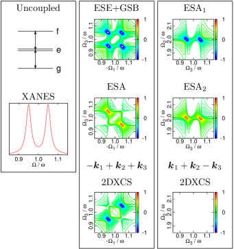
Figure 4: (Color online) XANES and 2DXCS (imaginary part) of a model four-level system representing two uncoupled core transitions. Left panel: The level scheme and XANES. Middle panel: The single- and double-resonance contributions and the total $\boldsymbol{k}_{I}$ 2DXCS. Right panel: Two double-resonance contributions and the total $\boldsymbol{k}_{III}$ 2DXCS.

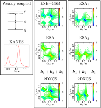
Figure 5: (Color online) Same as Fig. 4 but for a model four-level system representing two weakly-coupled core transitions.

In order to demonstrate the sensitivity of 2DXCS signals to the coupling between transitions, we have simulated the one-color ($\omega_{j}=\omega$) $\boldsymbol{k}_{I}$ and $\boldsymbol{k}_{III}$ signals for two model systems of uncoupled (Fig. 4) and weakly-coupled (Fig. 5) core transitions. We assumed broad bandwidth $\mathcal{E}^{+}(\omega_{fe_{j}}-\omega)\approx\mathcal{E}^{+}(\omega_{e_{j}g}-\omega)\approx 1$ for simplicity.

Using Eqs. (10)-(12) of Ref. Schweigert and Mukamel, 2008a, the one-color $-\boldsymbol{k}_{1}+\boldsymbol{k}_{2}+\boldsymbol{k}_{3}$ signal is given by

$$S_{I} (\Omega_{3},0,\Omega_{1})=S_{I}^{GSB}(\Omega_{3},0,\Omega_{1})+S_{I}^{ESE}(\Omega_{3},0,\Omega_{1})+S_{I}^{ESA}(\Omega_{3},0,\Omega_{1})$$ (7)

$$S_{I}^{GSB} (\Omega_{3},0,\Omega_{1})+S_{I}^{ESE}(\Omega_{3},0,\Omega_{1})$$

$$= \,\big{|}\mu_{ge_{1}}\big{|}^{2}\big{|}\mu_{ge_{1}}\big{|}^{2}\big{[}\frac{1}{\Omega_{1}+\omega_{e_{1}g}+i\Gamma_{e_{1}g}}+\frac{1}{\Omega_{1}+\omega_{e_{2}g}+i\Gamma_{e_{2}g}}\big{]}$$

$$\times\big{[}\frac{1}{\Omega_{3}-\omega_{e_{1}g}+i\Gamma_{e_{1}g}}+\frac{1}{\Omega_{3}-\omega_{e_{2}g}+i\Gamma_{e_{2}g}}\big{]}$$ (8)

$$S_{I}^{ESA} (\Omega_{3},0,\Omega_{1})$$

$$= \,-\frac{\mu_{ge_{1}}\mu_{e_{1}f}(\mu_{fe_{1}}\mu_{e_{1}g}+\mu_{fe_{2}}\mu_{e_{2}g})}{(\Omega_{1}+\omega_{e_{1}g}+i\Gamma_{e_{1}g})(\Omega_{3}-\omega_{e_{2}g}-\Delta+i\Gamma_{fe_{1}})}$$

$$-\frac{\mu_{ge_{2}}\mu_{e_{2}f}(\mu_{fe_{1}}\mu_{e_{1}g}+\mu_{fe_{2}}\mu_{e_{2}g})}{(\Omega_{1}+\omega_{e_{2}g}+i\Gamma_{e_{2}g})(\Omega_{3}-\omega_{e_{1}g}-\Delta+i\Gamma_{fe_{2}})}$$ (9)

where $\Delta$ is the anharmonicity of the single to double transition frequency

$$\omega_{fg}=\omega_{e_{1}g}+\omega_{e_{2}g}+\Delta$$ (10)

The $\boldsymbol{k}_{I}$ 2DXCS of a four-level system in general consists of two diagonal peaks at $(-\Omega_{1}=\omega_{e_{1}g},\Omega_{3}=\omega_{e_{1}g})$ and $(-\Omega_{1}=\omega_{e_{2}g},\Omega_{3}=\omega_{e_{2}g})$ and two off-diagonal cross peaks at $(-\Omega_{1}=\omega_{e_{1}g},\Omega_{3}=\omega_{e_{2}g})$ and $(-\Omega_{1}=\omega_{e_{2}g},\Omega_{3}=\omega_{e_{1}g})$. If two transitions are decoupled (Fig. 4, middle column), the spectrum is additive and the ESA contribution to the cross peaks cancels the ESE and GSB contributions and the cross peaks vanish. However, since the ESA term does not contribute to the diagonal peaks, they remain finite. If the two transitions are weakly-coupled (Fig. 5, middle column), the ESA contribution is red shifted by $\Delta$ resulting in two-lobe cross peak line shape. However, due to the destructive interference between the ESE/GSB and ESA terms, the cross peaks are much weaker than the diagonal peaks. Thus, for both decoupled and coupled transitions, high spectral resolution is necessary to distinguish the cross peak and extract the information about the couplings from the $\boldsymbol{k}_{I}$ spectrum.

Using Eq. (II), the one-color $\boldsymbol{k}_{1}+\boldsymbol{k}_{2}-\boldsymbol{k}_{3}$ 2DXCS signal in the broadband limit is recast as

$$S_{III} (\Omega_{3},\Omega_{2},0)$$

$$=\frac{\mu_{fe_{1}}\mu_{e_{1}g}+\mu_{fe_{2}}\mu_{e_{2}g}}{\Omega_{2}-\omega_{fg}+i\Gamma_{fg}}\big{[}$$

$$\times\frac{\mu_{ge_{1}}\mu_{e_{1}f}}{\Omega_{3}-\omega_{e_{1}g}+i\Gamma_{e_{1}g}}+\frac{\mu_{ge_{2}}\mu_{e_{2}f}}{\Omega_{3}-\omega_{e_{2}g}+i\Gamma_{e_{2}g}}$$

$$-\frac{\mu_{ge_{1}}\mu_{e_{1}f}}{\Omega_{3}-\omega_{e_{2}g}-\Delta+i\Gamma_{fe_{1}}}-\frac{\mu_{ge_{2}}\mu_{e_{2}f}}{\Omega_{3}-\omega_{e_{1}g}-\Delta+i\Gamma_{fe_{2}}}\big{]}$$ (11)

The spectrum of our four-level system thus consists of two pairs of peaks at $(\Omega_{3}=\omega_{e_{1}g},\Omega_{2}=\omega_{fg})$ and $(\Omega_{3}=\omega_{e_{2}g},\Omega_{2}=\omega_{fg})$. Both contributing pathways involve doubly-excited states, and the spectrum thus provides single-resonance-free probe of the couplings between the transitions. If the two core transitions are decoupled (Fig. 4, right column), then ESA₂ $=$ - ESA₁ and the total signal vanishes. If the two core transions are weakly coupled (Fig. 5, right column), the ESA₂ contribution is red shifted by $\Delta$, and the total spectrum exhibits two peaks each having the two-lobe structure similar to the $\boldsymbol{k}_{I}$ cross peaks. The splitting between the lobes is approximately equal to the anharmonicity.

IV Numerical simulations

2DXCS signals in molecules depend on states with two core-electrons excited. In all calculations, we used the singly and doubly-substituted Konh-Sham (KS) determinants in the equivalent-core approximation (refered to as DFT/ECA) to describe the necessary singly and doubly core-excited states. The expressions for the transition frequencies and dipole moments within this approximation were presented in Ref. Schweigert and Mukamel, 2008a. Doubly-substituted determinants are necessary to describe states in which the two core electrons are promoted to orbitals higher than the HOMO. The KS orbitals for the original and equivalent-core molecules where obtained with the combination of Becke’s exchangeBecke (1988) and Perdew’s correlationPerdew (1986) functionals and a combined basis set of Gaussian-type atomic orbitals, whereby an extensive IGLO-IIIKutzelnigg et al. (1991) set was used on N and a moderate 6-311G** setHehre et al. (1972) was used on all other atoms. The orbitals and their energies were calculated with the Gaussian 03 electronic structure code.Frisch et al.

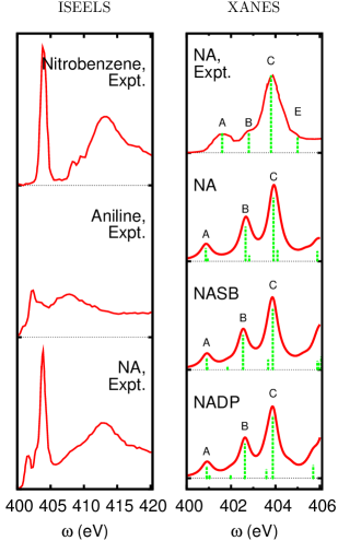
Figure 6: (Color online) Left panel: Experimental ISEELS of nitrobenzene, aniline, and NA from Ref. Turci et al., 1996. Right panel: Experimental ISEELS of NATurci et al. (1996), and present simulated XANES of NA, NASB, and NADP.

This computational protocol was tested by comparing the simulated N1s XANES of para-nitroaniline to experimental N1s inner-shell electron energy loss spectroscopy (ISEELS) of aniline, nitrobenzene, and para-nitroaniline from Ref. Turci et al., 1996. The experimental ISEELS are displayed on Fig. 6 (left panel). Under the experimental conditions in Ref. Turci et al., 1996 (high impact energy and small scattering angle) the ISEELS is expected to resemble XANES. The exprimental pre-edge ISEELS of para-nitroaniline (Fig. 6, right panel) consists of two weaker amine peaks at 401.6 eV and 402.6 eV, a strong nitroso peak at 403.8 eV, and amine peak at 405.0 eV. The measured core ionization potential is 406.0 eV.

The absorption edge (i.e., the frequency of the lowest transition) is given within the DFT/ECA as the energy difference between the core orbital in the original molecule and the HOMO energy in the equivalent-core molecules. This estimate however neglects the effect of the core-shell ionization on the remaining core electons. The relaxation among core electrons does not significantly affect the valence electrons, hence, its effect on XANES is limited to a shift of the entire spectrum. The core relaxation as well as relativistic effects contributing to the core-transition frequency can be corrected for by comparing with experiment. The nitroso N1s absorption edge in para-nitroaniline calculated within the ECA underestimates the experimental one by 21.7 eV. We further assumed that the core relaxation effects have the same magnitude for all system considered as well as the amine N 1s edge and thus shifted all the ECA core-transition frequencies by this value.

The main features of NA N1s XANES are qualitatively reproduced by the DFT/ECA method. The calculated XANES of para-nitroaniline (NA) overestimates the splitting between the lowest amine and the nitroso transitions (marked A and C in Fig. 6) predicting it to be 3.1 eV compared to experiment (2.2 eV). It also overestimates the second amine peak (marked B in Fig. 6) intensity. Also the experimental amine peak at 405.0 eV is not reproduced. Instead, the calculated XANES features weak peaks at 404 eV and 406 eV. In the the experimental spectrum these peaks may be covered by the strong nitroso peak.

The calculated XANES of 4-nitro-4$\prime$-aminestilbene (NASB, Fig. 6, right panel) and 4-nitro-4$\prime$-aminediphenyl (NADP, Fig. 6, right panel) are similar to NA and consist of an amine peaks at around 401.0 eV, stronger amine peaks at around 402.6 eV and the strongest nitroso peaks at arount 404.0 eV.

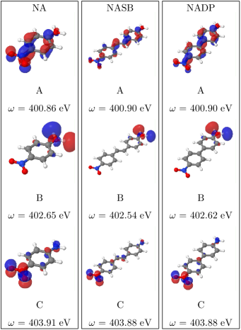
Figure 7: (Color online) Equivalent-core orbitals of NA, NASB, and NADP (as indicated) describing the promoted amine or nitroso 1s electron in singly-excited states with significant contribution to XANES.

Figure 7 shows the relevant ECA orbitals that give rise to the described features in the calculated XANES. The first amine peak in all three molecules involves promoting the 1s electron to the $\pi^{*}$ orbital of the conjugated system. Note that within the ECA, the core-hole potential is described by increasing the nuclear charge by 1, keeping the core-shell doubly-occupied, while an extra valence electron is added to describe the promoted core electron. The lowest ECA orbital is thus occupied and its shape resembles a bonding $\pi$ orbital rather then antibonding one. Two-ring NADP and NASB have another $\pi^{*}$-like orbital that gives rise to the very weak peak at 402.0 eV in the XANES spectra. The second strong amine peak arises due to the excitation of the amine 1s electron to the $\sigma^{*}$ orbital of the amine group.Finally, the strongest XANES feature at 404.0 eV arises due to transition of the nitroso 1s electron to the $\pi^{*}$ orbital, which mostly localized on the NO₂ group. The intensity of the 402.5 and 404.0 peaks can thus be explained by the fact that the corresponding ECA orbitals are strongly localized on the respective group.

We next turn to the N1s $\boldsymbol{k}_{III}$ signal obtained with four pulses of the same frequency $\omega_{j}=402.6eV$, the same temporal envelope, and linear polarization $\boldsymbol{e}_{j}=\boldsymbol{e}_{x}$. This one-color signal of a sample of randomly oriented molecules is given at $t_{1}=0$ by

$$S_{III}(\Omega_{3},\Omega_{2},t_{1}=0)= \sum_{e,e^{\prime},f}\mathcal{E}^{-}(\omega_{ge}+\omega)\mathcal{E}^{-}(\omega_{ef}+\omega)\mathcal{E}^{+}(\omega_{fe^{\prime}}-\omega)\mathcal{E}^{+}(\omega_{e^{\prime}g}-\omega)$$

$$\times\frac{\big{\langle}\mu_{fe^{\prime}}\mu_{e^{\prime}g}\mu_{ge}\mu_{ef}\big{\rangle}}{\Omega_{2}-\omega_{fg}+i\Gamma_{fg}}\bigg{[}\frac{1}{\Omega_{3}-\omega_{eg}+i\Gamma_{eg}}-\frac{1}{\Omega_{3}-\omega_{fe}+i\Gamma_{fe}}\bigg{]}$$ (12)

where $\big{\langle}\mu_{fe^{\prime}}\mu_{e^{\prime}g}\mu_{ge}\mu_{ef}\big{\rangle}$ is calculated as described in Appendix A.

We assume 100 attosecond rectangular pulse envelopes $\mathcal{E}_{j}(\omega)$ with 6 eV bandwidth around the carrier frequencies (i.e., $\mathcal{E}_{j}(\omega-\omega_{j})=1$ for $\big{|}\omega-\omega_{j}\big{|}\leq 3$ eV and zero otherwise). The same dephasing rate $\Gamma_{ab}=0.3$ eV is assumed for all transitions. Transitions to the continuum lie outside the chosen bandwidth and are neglected in the simulations.

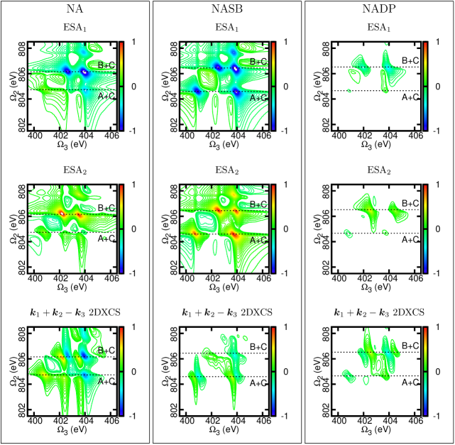
Figure 8: (Color online) Two ESA contributions and the total N1s $\boldsymbol{k}_{III}$ 2DXCS (imaginary part) of NA, NADP, and NASB.

$\boldsymbol{k}_{III}$ 2DXCS of NA, NADP and NASB are shown in Fig. 8. There are three core-excited states with significant dipole strength in the XANES of NA: two due to excitation of the amine core electron (states A and B) and one due to the excitation of the nitroso core electron (state C). The corresponding features in NA (Fig. 8, left panel) can be identified by their position along the $\Omega_{2}$ axis. The strongest feature is attributed to the doubly excited state corresponding to states B and C. The strong dipole coupling of each state results in a very strong individual ESA₁ and ESA₂ contributions. The negative inteference between the two pathways leads to the two peaks. The weaker dipole strength of the transition from to ground state to state A results in a weaker individual ESA₁ and ESA₂ contributions. However, due to the coupling between the A and C transitions, the transition dipole moment changes sign and the ESA₁ and ESA₂ pathways intefere constructively, resulting in a strong overall signal. Comparison of the equivalent-core orbitals describing the promoted core electron in the singly and doubly excited states (Fig. 7 and 9, left panels) explains the difference between the two sets of resonances. In state A, the promoted core electron is delocalized, hence states A and C states are strongly coupled, and the dipole coupling between the A states and the doubly excited state has opposite sign to the coupling between the C state and the doubly excited state. In contrast, state B is localized at the amine group, hence, the coupling between states B and C is weaker, and the overall signal is much smaller than each of the individual contributions.

Similar to NA, there are three core-excited states with significant dipole strength in the XANES of NASB: two due to excitation of the amine core electron (states A and B) and one due to the excitation of the nitroso core electron (state C). Given the similarity of the XANES spectra, the contributions ESA₁ and ESA₂ to NASB signal (Fig. 8, middle panel) are similar to NA. The strongest feature arises due to the double-excitation corresponding to states B and C. However, the total signal of NASB at $\Omega_{2}=806.4$ eV is much weaker than that of NA, which indicates that these states are uncoupled in the doubly-excited states. Analysis of the ECA orbitals (Fig. 7 and 9, middle panels) shows that indeed, the B state is strongly localized on the amine group. In NASB the amine and nitroso groups are separated by 12.3 A compared to 5.6 A in NA, hence the coupling between the B state (localized on amine group) and the C state (localized on the nitroso group) is much weaker than the coupling between these states in NA. State A is delocalized, and its coupling with state C is significant resulting in the characteristic two-lobe pattern.

The $\boldsymbol{k}_{III}$ spectrum of NADP is very weak (Fig. 8, right panel) with the maximum intensity approximately 5 times weaker than NA. This is surprising given that the electronic stucture of NADP is similar to NASB. Indeed, the equivalent-core orbitals describing the singly and doubly core excited states of NADP (Fig. 7 and 9, right panels) are similar to those of NASB. The single-orbital approximation would thus predict the 2DXCS signal stronger than in NASB due to the shorter distance between the two cores. Analysis of the calculated transition dipole moments shows however that the $\mu_{fe_{j}}\mu_{e_{j}g}$ factor (i.e., the probability amplitude of the two-photon excitation into doubly excited state $f$) is very small due to the cancellation between the transition moments describing excitations via two different core shells

$$\mu_{fe_{1}}\mu_{e_{1}g}+\mu_{fe_{2}}\mu_{e_{2}g}\approx 0$$ (13)

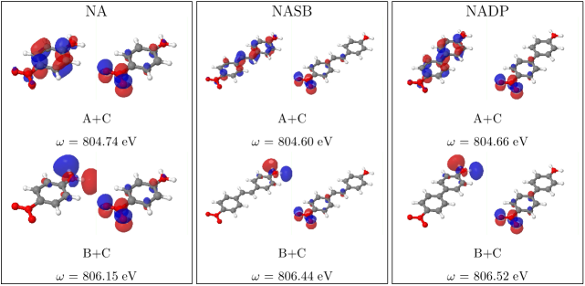
Figure 9: (Color online) Pairs of the equivalent-core orbitals of NA, NASB, and NADP (as indicated) describing the promoted amine and nitroso 1s electrons in doubly-excited states with significant contribution to the corresponding N1s $\boldsymbol{k}_{III}$ 2DXCS.

The lowest doubly excited state (marked A+C in Fig. 9, right panel) is described in the DFT/ECA approximation by a KS determinant where the $N+1$ orbital is occupied by the nitroso 1s electron and $N+2$ orbital is occupied by the amine electron. The corresponding two-photon transition amplitude is given in the ECA by Schweigert and Mukamel (2008a)

$$\mu_{fe_{1}} \mu_{e_{1}g}+\mu_{fe_{2}}\mu_{e_{2}g}=$$

$$\big{\langle}\phi^{(12)}_{N+2}\big{|}\hat{\mu}\big{|}\chi^{(1)}_{NH_{2}}\big{\rangle}\big{\langle}\phi^{(1)}_{N+1}\big{|}\hat{\mu}\big{|}\chi_{NO_{2}}\big{\rangle}\big{\langle}\Phi^{(12)}\big{|}\Phi^{(1)}\big{\rangle}\big{\langle}\Phi^{(1)}\big{|}\Phi\big{\rangle}$$

$$+\big{\langle}\phi^{(12)}_{N+1}\big{|}\hat{\mu}\big{|}\chi^{(2)}_{NO_{2}}\big{\rangle}\big{\langle}\phi^{(2)}_{N+1}\big{|}\hat{\mu}\big{|}\chi_{NH_{2}}\big{\rangle}\big{\langle}\Phi^{(12)}\big{|}\Phi^{(2)}\big{\rangle}\big{\langle}\Phi^{(2)}\big{|}\Phi\big{\rangle}$$ (14)

where $\chi_{NO_{2}}$, $\chi_{NH_{2}}$ are respectively the nitroso and amine N 1s orbitals, $\phi^{(12)}$, $\phi^{(2)}$, $\phi^{(1)}$ are the valence equivalent-core orbitals describing the promoted core electrons, and $\Phi^{(12)}$, $\Phi^{(2)}$, $\Phi^{(1)}$, $\Phi$ are the Slater determinants made of $N$ valence spectator orbitals in four equivalent-core molecules. In XANES, the one-electron transition dipole moments $\big{\langle}\phi^{(j)}\big{|}\hat{\mu}\big{|}\chi_{j}\big{\rangle}$ are often sufficient to qualitatively reproduce the experimental XANES intensities. Factors $\big{\langle}\Phi^{(j)}\big{|}\Phi\big{\rangle}$ describe the relaxation among the valence spectator orbitals, which often has a small effect on the computed XANES intensities. In case of NADP 2DXCS, however, the calculated overlap between the valence orbitals $\big{\langle}\Phi^{(12)}\big{|}\Phi^{(2)}\big{\rangle}$ and $\big{\langle}\Phi^{(12)}\big{|}\Phi^{(1)}\big{\rangle}$ have opposite sign,

$$\big{\langle}\Phi^{(12)}\big{|}\Phi^{(2)}\big{\rangle}\approx-\big{\langle}\Phi^{(12)}\big{|}\Phi^{(1)}\big{\rangle}$$ (15)

while the remaining quantities contributing to Eq. (IV) have the same sign and similar magnitude. Consequently, the probability amplitude of the corresponding two-photon excitation is much smaller than in NA or NASB. This is thus a purely many-body effect induced by relaxation among orbitals that are not directly participating in the core transitions. We note however that it is difficult to estimate the quality of the ECA in describing many-body effects such as the relaxation among the spectator orbitals. More accurate, many-body methods that explicitely describe core excitation and, ultimately, comparision with experimental data, may be needed to verify the effect of valence relaxation on 2DXCS signals.

V Conclusions

The double-quantum-coherence 2DXCS technique proposed here monitors the attosecond four-wave-mixing signal in the $\boldsymbol{k}_{III}$ phase-matching direction. The contribution of single resonances are eliminated and the signal consists only of peaks arising from the coupling between the core transitions in the doubly-excited states. Simulations were performed using sum-over-states expression derived using the rotating-wave approximation and include the pulse envelopes. The differences between $\boldsymbol{k}_{III}$ and $\boldsymbol{k}_{I}$ signals were demonstrated on a model four-level system with and without coupling between the transitions. Simulations of the N1s XANES and $\boldsymbol{k}_{III}$ spectra of para-nitroaniline and two-ring hydrocarbons disubstituted with an amine and a nitroso group showed that while XANES is virtually invariant to the differences in the molecular and electronic structure of these molecules, the double-quantum $\boldsymbol{k}_{III}$ technique is highly sensitive to the separation between the core-shell as well as the localization of the corresponding core-excited states.

Appendix A 2DXCS signal of an ensemble of randomly-oriented molecules

The first contribution to the $\boldsymbol{k}_{III}$ signal [Eq. (II)] is proportional to

$$\mu_{ge^{\prime}}^{4}\mu_{e^{\prime}f}^{3}\mu_{fe}^{2}\mu_{eg}^{1}=e_{4}^{\alpha_{4}*}e_{3}^{\alpha_{3}*}e_{2}^{\alpha_{2}}e_{1}^{\alpha_{1}}\mu_{ge^{\prime}}^{\alpha_{4}}\mu_{e^{\prime}f}^{\alpha_{3}}\mu_{fe}^{\alpha_{2}}\mu_{eg}^{\alpha_{1}}e^{-i\boldsymbol{k}_{4}\boldsymbol{r}_{4}-i\boldsymbol{k}_{3}\boldsymbol{r}_{3}+i\boldsymbol{k}_{2}\boldsymbol{r}_{2}+i\boldsymbol{k}_{1}\boldsymbol{r}_{1}}$$ (16)

where $\alpha_{j}$ refers to the laboratory-frame Cartesian components of the $j$th pulse polarization vector and the corresponding dipole transition moment, and $\boldsymbol{r}_{j}$ is the laboratory-frame position of the core-shell interacting with the $j$th pulse.

The transition dipole moments are calculated in the molecular frame and thus must be transformed to the laboratory frame

$$\mu_{ge^{\prime}}^{\alpha_{4}}\mu_{e^{\prime}f}^{\alpha_{3}}\mu_{fe}^{\alpha_{2}}\mu_{eg}^{\alpha_{1}}=I^{\alpha_{1}\alpha_{2}\alpha_{3}\alpha_{4}}_{\beta_{1}\beta_{2}\beta_{3}\beta_{4}}\mu_{ge^{\prime}}^{\beta_{4}}\mu_{e^{\prime}f}^{\beta_{3}}\mu_{fe}^{\beta_{2}}\mu_{eg}^{\beta_{1}}$$ (17)

Here, $\beta_{n}$ refers to the Cartesian components of the dipole transition moments in the molecular frame. $I^{\alpha_{1}\alpha_{2}\alpha_{3}\alpha_{4}}_{\beta_{1}\beta_{2}\beta_{3}\beta_{4}}$ is the product of the four directional cosines of the angles between the laboratory axes $\alpha_{n}$ and molecular axes $\beta_{n}$ Andrews and Thirunamachandran (1977).

The index $f$ refers to states with two core electrons excited. If $e^{\prime}=e$, we have $\boldsymbol{r}_{4}=\boldsymbol{r}_{1}$ and $\boldsymbol{r}_{2}=\boldsymbol{r}_{3}$ and

$$e^{-i\boldsymbol{k}_{4}\boldsymbol{r}_{4}-i\boldsymbol{k}_{3}\boldsymbol{r}_{3}+i\boldsymbol{k}_{2}\boldsymbol{r}_{2}+i\boldsymbol{k}_{1}\boldsymbol{r}_{1}}=\left\{\begin{array}[]{ll}e^{i(\boldsymbol{k}_{1}-\boldsymbol{k}_{4})(\boldsymbol{r}_{1}-\boldsymbol{r}_{2})},&\forall e^{\prime}=e\\ e^{i(\boldsymbol{k}_{1}-\boldsymbol{k}_{3})(\boldsymbol{r}_{1}-\boldsymbol{r}_{2})},&\forall e^{\prime}\neq e\\ \end{array}\right.$$ (20)

where we used the fact that the 2DXCS signal is measured under the phase matching condition, $\boldsymbol{k}_{1}+\boldsymbol{k}_{2}-\boldsymbol{k}_{3}-\boldsymbol{k}_{4}=0$.

$$e^{-i\boldsymbol{k}_{4}\boldsymbol{r}_{4}-i\boldsymbol{k}_{3}\boldsymbol{r}_{3}+i\boldsymbol{k}_{2}\boldsymbol{r}_{2}+i\boldsymbol{k}_{1}\boldsymbol{r}_{1}}=e^{i2\pi q(L/\lambda)cos(\theta)}$$ (21)

where $\theta$ is the angle between the vectors $\boldsymbol{k}_{1}-\boldsymbol{k}_{3}$ and $\boldsymbol{r}_{1}-\boldsymbol{r}_{2}$, $q=\big{|}\boldsymbol{k}_{1}-\boldsymbol{k}_{3}\big{|}/\big{|}\boldsymbol{k}_{1}\big{|}$, and $L$ is the distance between the two core shells contributing to the signal. Here, $\theta$ depends on the orientation of the molecule in the laboratory frame, and $q$ ($0\leq q\leq 2$) depends on the pulse configuration.

$$\mu_{ge^{\prime}}^{4}\mu_{e^{\prime}f}^{3}\mu_{fe}^{2}\mu_{eg}^{1}=\mu_{ge^{\prime}}^{\beta_{4}}\mu_{e^{\prime}f}^{\beta_{3}}\mu_{fe}^{\beta_{2}}\mu_{eg}^{\beta_{1}}\big{\langle}e^{i2\pi q(L/\lambda)\cos(\theta)}I^{XXXX}_{\beta_{1}\beta_{2}\beta_{3}\beta_{4}}\big{\rangle}$$ (22)

The distance between the N and O atoms in NASB, the largest molecule considered, is $\approx$ 12 Å. Assuming $q\approx 1$, the prefactor is $e^{i\pi/3\cos(\theta)}$ and its contribution to the averaged signal is expected to be small. In our calculations we neglected it and used the following expression for the XXXX pulse configuration

$$\mu_{ge^{\prime}}^{4}\mu_{e^{\prime}f}^{3}\mu_{fe}^{2}\mu_{eg}^{1}=-\frac{1}{15}\big{[}\mu_{ge^{\prime}}^{\beta_{2}}\mu_{e^{\prime}f}^{\beta_{2}}\mu_{fe}^{\beta_{1}}\mu_{eg}^{\beta_{1}}+\mu_{ge^{\prime}}^{\beta_{2}}\mu_{e^{\prime}f}^{\beta_{1}}\mu_{fe}^{\beta_{2}}\mu_{eg}^{\beta_{1}}+\mu_{ge^{\prime}}^{\beta_{2}}\mu_{e^{\prime}f}^{\beta_{1}}\mu_{fe}^{\beta_{1}}\mu_{eg}^{\beta_{2}}\big{]}$$ (23)

Since the third and the fourth pulse have identical polarization, the second term contributing to Eq. (II) is similarly given by Eq. (23).

Figure 1: Molecular structure of 4-nitroaniline (NA), 4-nitro-4$\prime$-aminestilbene (NASB), and 4-nitro-4$\prime$-aminediphenyl (NADP)

Figure 3: Double-side Feynman diagrams representing the two contributions to the $\boldsymbol{k}_{III}=\boldsymbol{k}_{1}+\boldsymbol{k}_{2}-\boldsymbol{k}_{3}$ signal [Eq. (II)].

References

- Stohr (1996) J. Stohr, NEXAFS Spectroscopy (Springer, New York, 1996).
- Mukamel (2000) S. Mukamel, Annu. Rev. Phys. Chem. 51, 691 (2000).
- Mukamel and Hochstrasser (2001) S. Mukamel and R. Hochstrasser, eds., Special Issue on Multidimensional Spectroscopies, vol. 266 of Chem. Phys. (2001).
- Jonas (2003) D. M. Jonas, Annu. Rev. Phys. Chem. 54, 425 (2003).
- Engel et al. (2007) G. S. Engel, T. R. Calhoun, E. L. Read, T. K. Ahn, T. Mancal, Y. C. Cheng, R. E. Blankenship, and G. R. Fleming, Nature 446, 782 (2007).
- Hochstrasser (2007) R. M. Hochstrasser, Proc. Natl. Acad. Sci. USA 104, 14189 (2007).
- Li et al. (2006) X. Li, T. Zhang, C. N. Borca, and S. T. Cundiff, Phys. Rev. Lett. 96, 057406 (2006).
- Chernyak et al. (1998) V. Chernyak, W. M. Zhang, and S. Mukamel, J. Chem. Phys. 109, 9587 (1998).
- Zhang et al. (1999) W. Zhang, V. Chernyak, and S. Mukamel, J. Chem. Phys. 110, 5011 (1999).
- Bucksbaum (2007) P. H. Bucksbaum, Science 317, 766 (2007).
- Goulielmakis et al. (2007) E. Goulielmakis, V. S. Yakovlev, A. L. Cavalieri, M. Uiberacker, V. Pervak, A. Apolonski, R. Kienberger, U. Kleineberg, and F. Krausz, Science 317, 769 (2007).
- Kapteyn et al. (2007) H. Kapteyn, O. Cohen, I. Christov, and M. Murnane, Science 317, 775 (2007).
- Brown et al. (1999) F. L. H. Brown, K. R. Wilson, and J. Cao, J. Chem. Phys. 111, 6238 (1999).
- Gel’mukhanov et al. (2000) F. Gel’mukhanov, P. Cronstrand, and H. Agren, Phys.Rev. A 61, 2503 (2000).
- Privalov et al. (2003) T. Privalov, F. Gel’mukhanov, and H. Agren, J. Electron Spectrosc. Relat. Phenom. 129, 43 (2003).
- Bressler and Chergui (2004) C. Bressler and M. Chergui, Chem. Rev. 104, 1781 (2004).
- Campbell and Mukamel (2004) L. Campbell and S. Mukamel, J. Chem. Phys. 121, 12323 (2004).
- Tanaka and Mukamel (2002a) S. Tanaka and S. Mukamel, Phys. Rev. Lett. 89, 043001 (2002a).
- Tanaka and Mukamel (2002b) S. Tanaka and S. Mukamel, J. Chem. Phys. 116, 1877 (2002b).
- Guimaraes et al. (2004) F. F. Guimaraes, V. Kimberg, F. Gel’mukhanov, and H. Agren, Phys. Rev. A 70, 062504 (2004).
- Tanaka and Mukamel (2004) S. Tanaka and S. Mukamel, J. Electron Spectrosc. Relat. Phenom. 136, 185 (2004).
- Felicissimo et al. (2005) V. C. Felicissimo, F. F. Guimaraes, F. Gel’mukhanov, A. Cesar, and H. Agren, J. Chem. Phys. 122, 094319 (2005).
- Guimaraes et al. (2005) F. F. Guimaraes, V. Kimberg, V. C. Felicissimo, F. Gel’mukhanov, A. Cesar, and H. Agren, Phys. Rev. A 71, 043407 (2005).
- Liu et al. (2008) J.-C. Liu, Y. Velkov, Z. Rinkevicius, H. Agren, and F. Gel’mukhanov, Phys. Rev. A 77, 043405 (2008).
- Tanaka and Mukamel (2003) S. Tanaka and S. Mukamel, Phys. Rev. A 67, 033818 (2003).
- Schweigert and Mukamel (2007a) I. V. Schweigert and S. Mukamel, Phys. Rev. A 76, 012504 (2007a).
- Mukamel (2005) S. Mukamel, Phys. Rev. B 72, 235110 (2005).
- Schweigert and Mukamel (2007b) I. V. Schweigert and S. Mukamel, Phys. Rev. Lett. 99, 163001 (2007b).
- Schweigert and Mukamel (2008a) I. V. Schweigert and S. Mukamel, J. Chem. Phys. 182, 184307 (2008a).
- Healion et al. (in press) D. M. Healion, I. V. Schweigert, and S. Mukamel, J. Phys. Chem. A (in press).
- Scheurer and Mukamel (2001) S. Scheurer and S. Mukamel, J. Chem. Phys. 115, 4989 (2001).
- Ernst et al. (1987) R. Ernst, G. Bodenhausen, and A. Wokaun, Principles of Nuclear Magnetic Resonance in One and Two Dimensions (Claredon Press: Oxford, 1987).
- Cervetto et al. (2004) V. Cervetto, J. Helbing, J. Bredenbeck, and P. Hamm, J. Chem. Phys. 121, 5935?5942 (2004).
- Fulmer et al. (2004) E. Fulmer, P. Mukherjee, A. Krummel, and M. Zanni, J. Chem. Phys. 120, 8067 (2004).
- Zhuang et al. (2005) W. Zhuang, D. Abramavicius, and S. Mukamel, Proc. Natl. Acad. Sci. USA 102, 7443?7448 (2005).
- Li et al. (2008) Z. Li, D. Abramavicius, and S. Mukamel, J. Am. Chem. Soc. 130, 3509 (2008).
- Abramavicius et al. (2008) D. Abramavicius, D. V. Voronine, and S. Mukamel, Proc. Natl. Acad. Sci. USA 105, 8525 (2008).
- Mukamel (1995) S. Mukamel, Principles of Nonlinear Optical Spectroscopy (Oxford University Press, New York, 1995).
- Schweigert and Mukamel (2008b) I. V. Schweigert and S. Mukamel, Phys. Rev. A 77, 033802 (2008b).
- Becke (1988) A. D. Becke, Phys. Rev. A 38, 3098 (1988).
- Perdew (1986) J. P. Perdew, Phys. Rev. B 33, 8822 (1986).
- Kutzelnigg et al. (1991) W. Kutzelnigg, U. Fleischer, and M. Schindler, The IGLO-Method: Ab Initio Calculation and Interpretation of NMR Chemical Shifts and and Magnetic Susceptibilities, vol. vol. 23 of NMR Basic Principles and Progress (Springer-Verlag, Heidelberg, 1991).
- Hehre et al. (1972) W. J. Hehre, R. Ditchfield, and J. A. Pople, J. Chem. Phys. 56, 2257 (1972).
- (44) M. J. Frisch, G. W. Trucks, H. B. Schlegel, G. E. Scuseria, M. A. Robb, J. R. Cheeseman, J. A. Montgomery, Jr., T. Vreven, K. N. Kudin, J. C. Burant, et al., Gaussian 03, revision c.02, gaussian, Inc., Wallingford, CT, 2004.
- Turci et al. (1996) C. C. Turci, S. G. Urquhart, and A. P. Hitchcock, Can. J. Chem.-Rev. Can. Chim. 74, 851 (1996).
- Andrews and Thirunamachandran (1977) D. L. Andrews and T. Thirunamachandran, J. Chem. Phys. 67, 5026 (1977).